Recurrent Memory: Extending Transformer Context with Segment-Level State Caching

Transformers process sequences in fixed-length segments. When a document exceeds the context window, the standard approach is to truncate or split it, processing each piece independently. But this independence comes at a cost: information from earlier segments vanishes entirely. A pronoun in segment 3 cannot resolve to its antecedent in segment 1 because segment 1 no longer exists in the model's view.

Transformer-XL introduced a solution that seems almost obvious in retrospect: what if we kept the hidden states from the previous segment and let the current segment attend to them? This segment-level recurrence creates a form of memory that extends effective context far beyond the training sequence length. The model processes sequences one segment at a time, but each segment can "remember" what came before through cached hidden states.

This chapter explores how Transformer-XL implements recurrent memory, why it requires relative positional encodings, and what limitations remain. Understanding this approach illuminates a key tension in long-context modeling: the tradeoff between computational efficiency and true bidirectional context.

Standard transformers suffer from what the Transformer-XL paper calls "context fragmentation." When you split a long document into fixed-length segments, each segment is processed without any knowledge of its neighbors. The model sees each chunk as an independent sequence.

Consider processing a 4096-token document with a 512-token context window. The naive approach splits this into 8 segments, processing each independently. Token 513 (the first token of segment 2) cannot attend to token 512 (the last token of segment 1). They're as disconnected as tokens from completely different documents.

Less than 13% of potential token-to-token dependencies are visible when processing with context fragmentation. Cross-segment dependencies, which may carry crucial information like coreference chains or long-range discourse structure, are completely invisible.

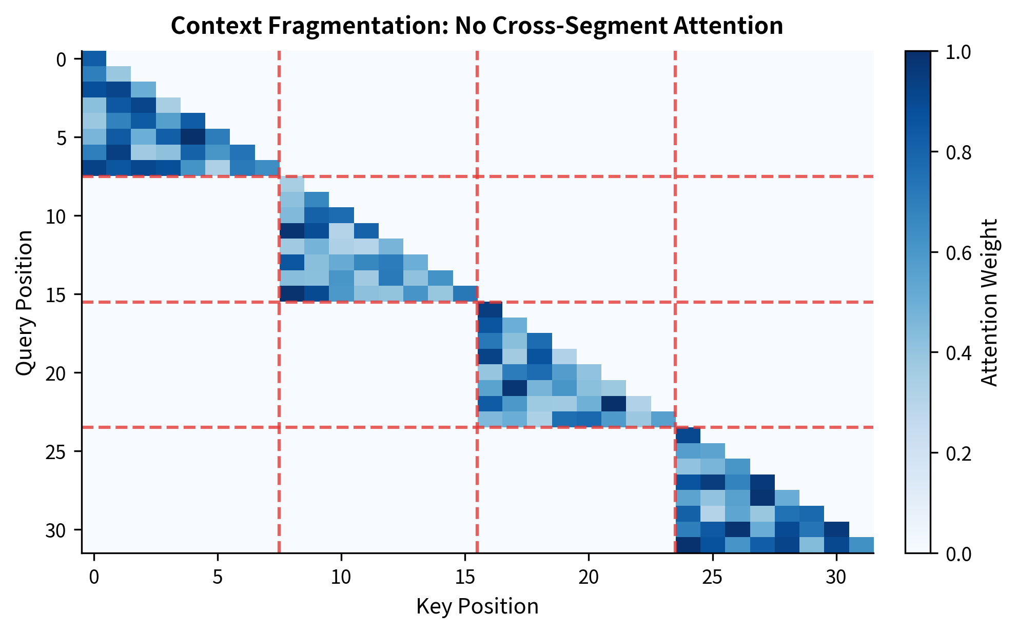
The attention pattern reveals the fundamental limitation: each segment is an island. No matter how important a reference in segment 1 might be for understanding segment 4, that information cannot flow through the attention mechanism.

Now that we understand the problem, let's explore how Transformer-XL solves it. The solution is remarkably simple: instead of discarding the previous segment entirely, cache its hidden states and make them available during attention computation for the current segment.

Think of it like this: when you read a new paragraph, you don't forget the previous one. You carry forward a mental summary of what came before. That summary isn't the original words themselves, but your processed understanding of them. Transformer-XL does exactly this, but with hidden states instead of mental summaries.

The recurrence operates at each layer independently. When processing layer $n$ of segment $\tau$, the model:

1. Retrieves the cached hidden states $\mathbf{h}_{\tau-1}^{n-1}$ from processing the previous segment at layer $n-1$
2. Concatenates these cached states with the current segment's hidden states
3. Computes attention where queries come only from the current segment, but keys and values span both the cached and current states
4. Caches the current segment's output hidden states for use when processing the next segment

This creates an asymmetric attention pattern: current tokens can "look back" at cached tokens, but we never recompute outputs for the cached tokens. They're frozen representations from the previous forward pass.

Let's formalize this mechanism. Suppose we're processing segment $\tau$, which contains $L$ tokens. The previous segment's hidden states, also of length $L$ (or some memory length $M$), have been cached. At layer $n$, we want to compute attention over an extended context that includes both segments.

The extended context for attention at layer $n$ is:

where:

• $\tilde{\mathbf{h}}_\tau^{n-1}$: the extended hidden states combining previous and current segments
• $\mathbf{h}_{\tau-1}^{n-1}$: cached hidden states from the previous segment at layer $n-1$
• $\mathbf{h}_\tau^{n-1}$: current segment's hidden states at layer $n-1$
• $\text{StopGrad}(\cdot)$: stops gradient flow to prevent backpropagating through the cached states
• $\circ$: concatenation along the sequence dimension

The attention computation then becomes:

where:

• $\mathbf{q}_\tau^n \in \mathbb{R}^{L \times d}$: queries from the current segment only
• $\mathbf{k}_\tau^n, \mathbf{v}_\tau^n \in \mathbb{R}^{(L + M) \times d}$: keys and values from the extended context (current + cached)
• $W_q^n, W_k^n, W_v^n$: learnable projection matrices for layer $n$
• $M$: the length of the cached memory (typically equal to segment length $L$)

The critical detail is that queries come only from the current segment while keys and values include the cached previous segment. This asymmetry is intentional: we want current tokens to attend to past context, but we don't want to regenerate outputs for past tokens. The cached states are read-only: they provide context but don't receive updates.

Let's translate this into code. The core operation is straightforward: concatenate cached and current hidden states, project to queries/keys/values, and compute attention with appropriate masking.

The output shows that token 0 of the current segment allocates substantial attention to the cached memory. This is expected: with no preceding tokens in the current segment, the memory provides all available context. The attention weights reveal how information flows. The first token in the current segment can attend to all 8 cached tokens plus itself. Later tokens in the current segment can attend to even more context: all cached tokens plus all preceding tokens in the current segment.

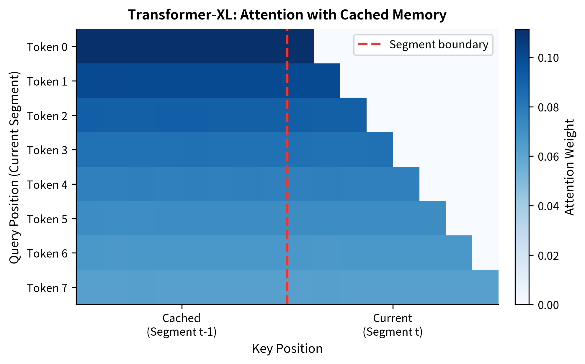
The attention pattern shows the distinctive Transformer-XL signature: a triangular pattern in the current segment (causal self-attention) combined with a rectangular region on the left (attention to cached memory). Every token in the current segment can see the entire cached memory.

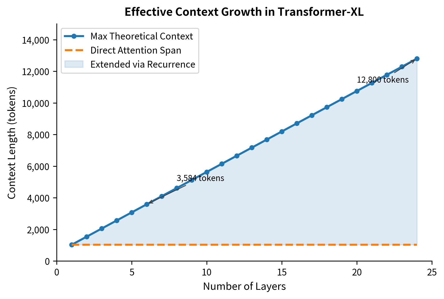
The recurrence mechanism creates a dependency chain across segments. Information from segment 1 flows to segment 2 through the cached hidden states. Segment 2's hidden states then carry forward information to segment 3. This chain means the effective context length grows beyond a single segment, bounded by how far information can propagate through the hidden states.

For an $N$-layer transformer with segment length $L$, the maximum effective context length is $O(N \times L)$. To understand why, consider how information propagates layer by layer:

• Layer 1 of segment $\tau$ receives cached states from layer 0 of segment $\tau - 1$, giving it access to 1 previous segment
• Layer 2 of segment $\tau$ receives cached states from layer 1 of segment $\tau - 1$, which already incorporated information from segment $\tau - 2$ at its own layer 1
• Layer $n$ can potentially access information from $n$ segments back through this chain of cached representations

The depth of the network acts as a multiplier on the effective context window.

A 24-layer model with 512-token segments can theoretically access information from over 13,000 tokens ago, even though it only directly attends to 1,024 tokens per layer. The depth of the network amplifies the effective context.

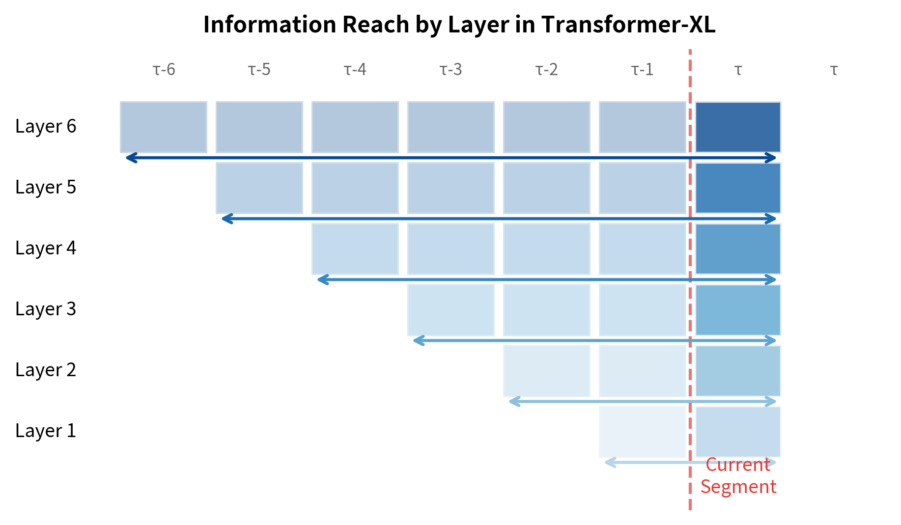
The visualization shows how context reach expands with network depth. Layer 1 can only see the immediately preceding segment through cached states. Layer 6, however, has access to information from 6 segments back because the cached states at layer 5 already incorporated information that propagated through the previous segment's entire network.

Standard absolute position encodings break under segment-level recurrence. If we use learned or sinusoidal position embeddings based on absolute positions within each segment, we encounter a fundamental inconsistency.

Consider a token at position 5 in segment $\tau$. In the previous segment $\tau - 1$, there was also a token at position 5. Both receive the same absolute position encoding. But from the perspective of the current segment, these tokens are at very different distances: position 5 in the current segment is "here," while position 5 in the cached segment is 8 positions back (if segments have length 8).

If absolute position encodings were used, the model would receive conflicting signals. Two tokens with identical position encodings would be at different temporal distances. The attention mechanism, which relies on position information to understand sequence structure, would be confused.

Transformer-XL solves this with relative position encodings. Instead of encoding absolute positions and adding them to token embeddings, the model directly encodes the relative distance between query and key positions in the attention computation itself.

We've established that segment-level recurrence breaks absolute position encodings. A token at position 5 in the cached segment and position 5 in the current segment have the same absolute encoding, yet they are 8 positions apart from the perspective of the current segment. How do we fix this? The answer lies in rethinking what position information attention actually needs.

When you read a sentence like "The cat sat on the mat because it was tired," you understand that "it" refers to "cat" not because of their absolute positions in the document, but because of their relative proximity. The pronoun comes shortly after its antecedent. This observation is the key insight: attention cares about how far apart tokens are, not where they are in absolute terms.

Consider two identical queries, one at position 10 and one at position 100, both attending to keys that are 3 positions before them. If the tokens involved have the same content, shouldn't these attention computations behave similarly? With absolute position encodings, they don't, because positions 7 and 97 have completely different encodings. With relative position encodings, they do, because "3 positions back" always means the same thing.

To understand how Transformer-XL achieves relative position encoding, we need to first dissect how position information enters standard attention. In the original transformer, the attention score between a query at position $i$ and a key at position $j$ starts as a simple dot product:

where:

• $\text{score}_{ij}$: the attention score determining how much position $i$ attends to position $j$
• $\mathbf{q}_i$: the query vector at position $i$
• $\mathbf{k}_j$: the key vector at position $j$

But where does position come in? The original transformer adds position embeddings to token embeddings before projecting to queries and keys. So the query at position $i$ is actually $W_q(\mathbf{x}_i + \mathbf{p}_i)$ and the key at position $j$ is $W_k(\mathbf{x}_j + \mathbf{p}_j)$. Substituting these into the dot product:

where:

• $\mathbf{x}_i, \mathbf{x}_j$: token embeddings at positions $i$ and $j$
• $\mathbf{p}_i, \mathbf{p}_j$: absolute position embeddings for positions $i$ and $j$
• $W_q, W_k$: learnable query and key projection matrices

This is where the magic of algebra reveals hidden structure. When we expand this product using the distributive property, we get four distinct terms:

Each term tells us something different about why one token might attend to another:

• Content-content: "Does this token's meaning relate to that token's meaning?" This is pure semantic matching, independent of where the tokens appear.
• Content-position: "Given what this token is looking for, does that position matter?" For example, a verb might preferentially attend to its subject, which typically precedes it.
• Position-content: "Given where this token is, does that token's content matter more?" Early positions might attend differently than late positions.
• Position-position: "Do these two positions have an inherent affinity?" Adjacent positions might naturally attend to each other.

The problem with this decomposition is that all position information uses absolute positions $\mathbf{p}_i$ and $\mathbf{p}_j$. Transformer-XL's insight is that we can rewrite these terms to use relative position instead. The redesign makes two key changes:

1. Replace the key's absolute position with relative distance: Instead of $\mathbf{p}_j$ (the absolute position of the key), use $\mathbf{r}_{i-j}$ (the relative distance from query to key).

2. Replace the query's position with a learned global bias: The query's absolute position $\mathbf{p}_i$ becomes learned vectors $\mathbf{u}$ and $\mathbf{v}$ that don't depend on position at all.

The resulting formula is:

Let's unpack each component:

• $\mathbf{x}_i, \mathbf{x}_j$: token embeddings at positions $i$ and $j$, unchanged from before
• $\mathbf{r}_{i-j}$: a sinusoidal encoding of the relative distance $i - j$, not the absolute position
• $W_{k,E}$: key projection matrix for content (the "E" stands for embeddings)
• $W_{k,R}$: key projection matrix for relative positions (the "R" stands for relative)
• $\mathbf{u}$: a learned global bias for content attention, shared across all query positions
• $\mathbf{v}$: a learned global bias for position attention, also shared across all positions

Why does this work? Consider what each term now captures:

1. Term (a): Pure content-based attention. This is unchanged from standard attention. The word "cat" attends to "feline" because of semantic similarity, regardless of position.

2. Term (b): Content-dependent distance preference. The query content determines how much the model cares about distance. A pronoun might strongly prefer nearby tokens, while a discourse marker might look further back.

3. Term (c): Global content importance. Some tokens are just important regardless of the query's position. The beginning-of-sentence token might receive attention from everywhere.

4. Term (d): Global distance preference. The model learns a general preference for certain distances. Typically, nearby tokens receive more attention than distant ones.

The crucial insight is that terms (b) and (d) now depend on $i - j$ rather than on $i$ and $j$ separately. This means the position signal is the same whether we're at the start of the document or the end, whether we're attending within the current segment or reaching back into cached memory.

With the theory in place, let's implement relative position encoding step by step. We need two components: (1) a function to generate sinusoidal encodings for each possible relative distance, and (2) a function to compute attention scores using the four-term formula.

The sinusoidal encoding for relative positions works similarly to absolute position encodings, but instead of encoding absolute positions 0, 1, 2, ..., we encode relative distances ..., -2, -1, 0, 1, 2, .... Negative distances mean the key is before the query; positive distances mean the key is after the query (though in causal attention, we only see non-positive distances).

The scores vary based on both content similarity and relative distance. Notice that the scores to cached positions (which are further away) differ from scores to current positions (which are closer). The relative position encoding ensures consistent treatment of distance regardless of absolute segment boundaries. A token attending to something 3 positions back receives the same position signal whether that's within the current segment or reaching into the cached memory.

To better understand how these four terms contribute to the final attention score, let's decompose them for a single query-key pair across different relative distances:

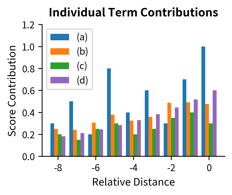
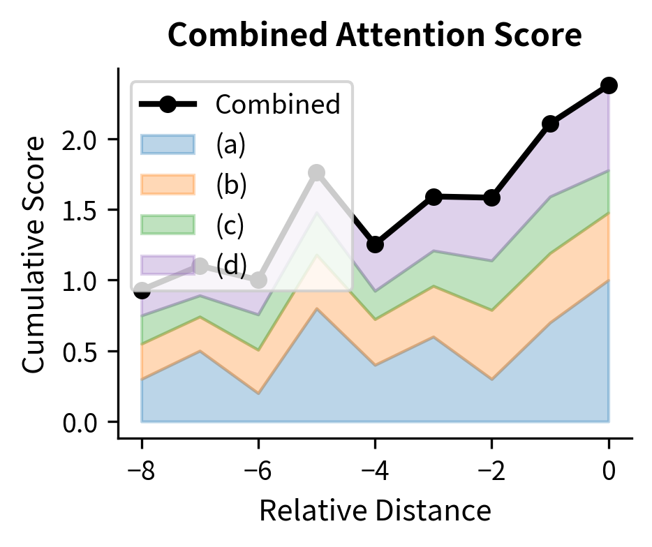
The visualization shows how content similarity (term a) provides the base signal, while position terms (b, c, d) modulate attention based on distance. The strong preference for position 0 (self-attention) reflects both high content similarity and the global position bias favoring nearby tokens.

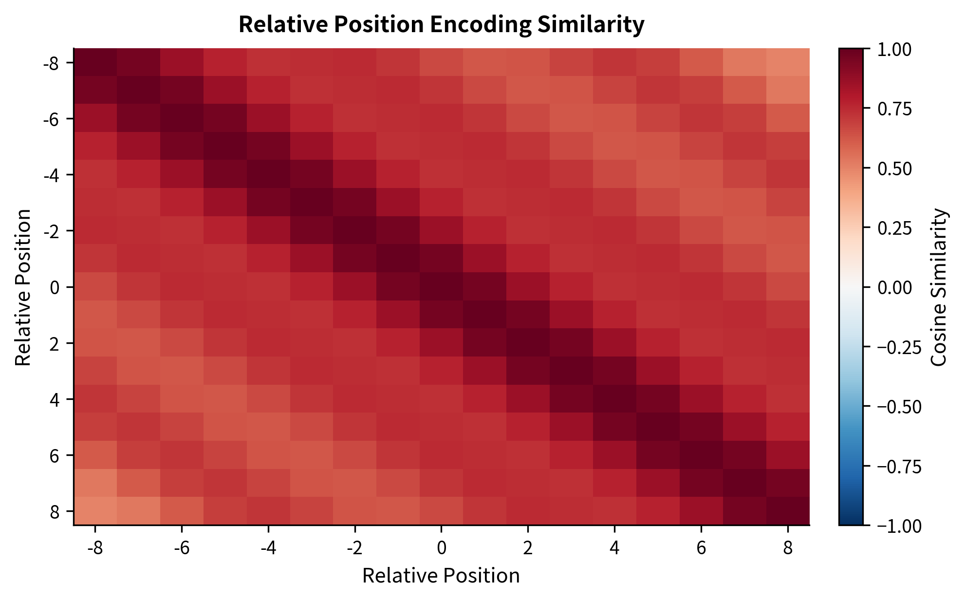
The similarity matrix shows that encodings for nearby relative positions are similar, gradually diverging for larger distances. This smooth decay allows the attention mechanism to naturally prefer nearby tokens while still accessing distant context when needed.

We've now covered the two core innovations of Transformer-XL: segment-level recurrence for extending context across segment boundaries, and relative position encoding for handling positions consistently across segments. Let's bring these pieces together into a complete implementation.

A Transformer-XL layer follows the same structure as a standard transformer layer: attention followed by feed-forward, with residual connections and layer normalization. The key differences are in the attention computation, where we must handle cached memory and compute relative position biases.

The attention shape for segment 2 is (8, 16), reflecting 8 query positions attending to 16 key positions (8 cached + 8 current). The total attention sums show how much of the model's attention budget goes to memory versus the current segment. A roughly balanced split indicates the model is actively using both sources of context.

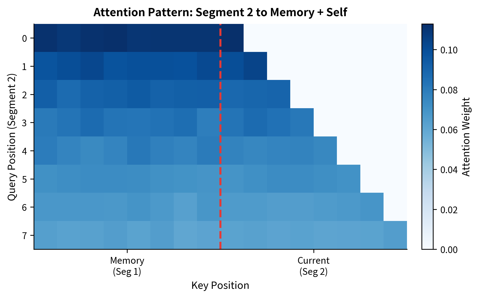
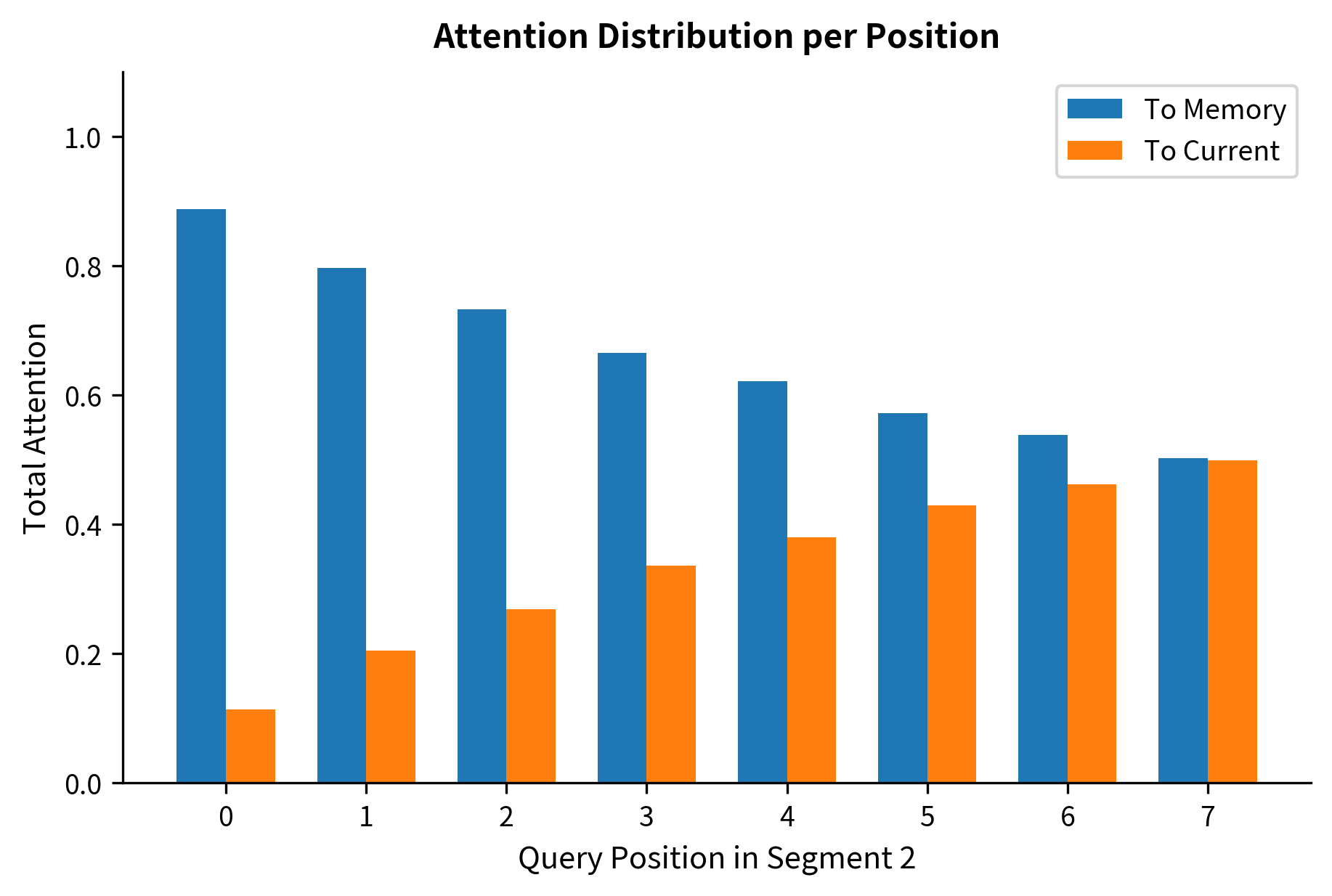
The visualization reveals how attention is distributed between memory and the current segment. Early positions in the current segment allocate substantial attention to memory because they have limited local context. Later positions can attend more to the growing local context while still accessing memory for longer-range dependencies.

How does Transformer-XL's approach compare to other long-context methods? We can evaluate on a synthetic task that explicitly requires long-range dependencies: the copying task. The model must reproduce a sequence of tokens after a long delay filled with noise.

This copying task becomes impossible for models without sufficient context. If the segment length is 100 and the delay is 200, a standard transformer with context fragmentation can never succeed because the tokens to copy fall outside any segment that needs to reproduce them.

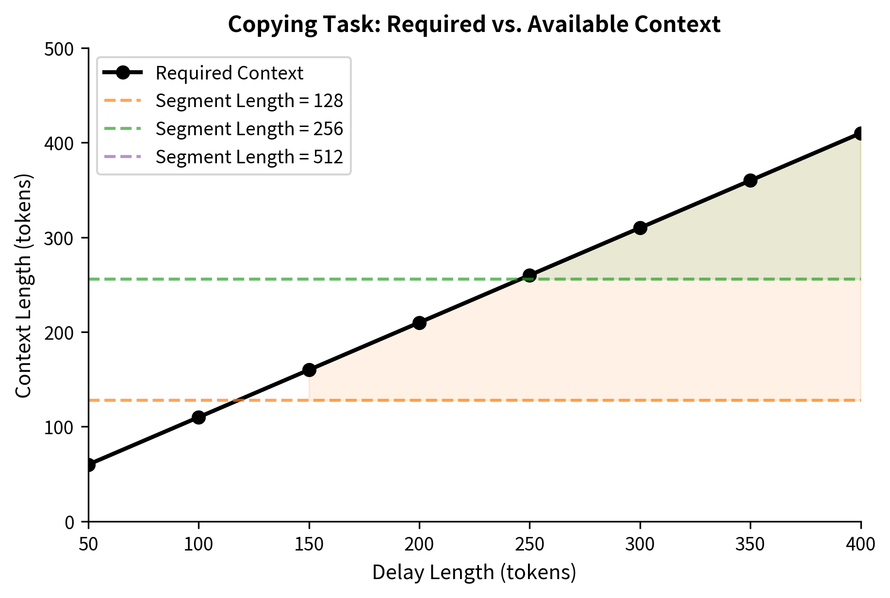
The figure illustrates the fundamental limitation of fixed context windows. As delay length increases, the required context eventually exceeds any fixed segment length. Standard transformers fail in the shaded regions. Transformer-XL extends the failure threshold by a factor proportional to the number of layers, but the memory cache size and information decay still impose practical limits.

While Transformer-XL's segment-level recurrence significantly extends effective context, it comes with important limitations that shape when and how the technique should be applied.

Information decay over segments. Hidden states are finite-dimensional vectors. As information propagates through multiple segments, it inevitably compresses and degrades. A fact stated in segment 1 may be perfectly preserved in segment 2's hidden states, partially preserved in segment 3, and largely lost by segment 10. Unlike attention over the full sequence, recurrence cannot perfectly preserve arbitrary information over arbitrary distances.

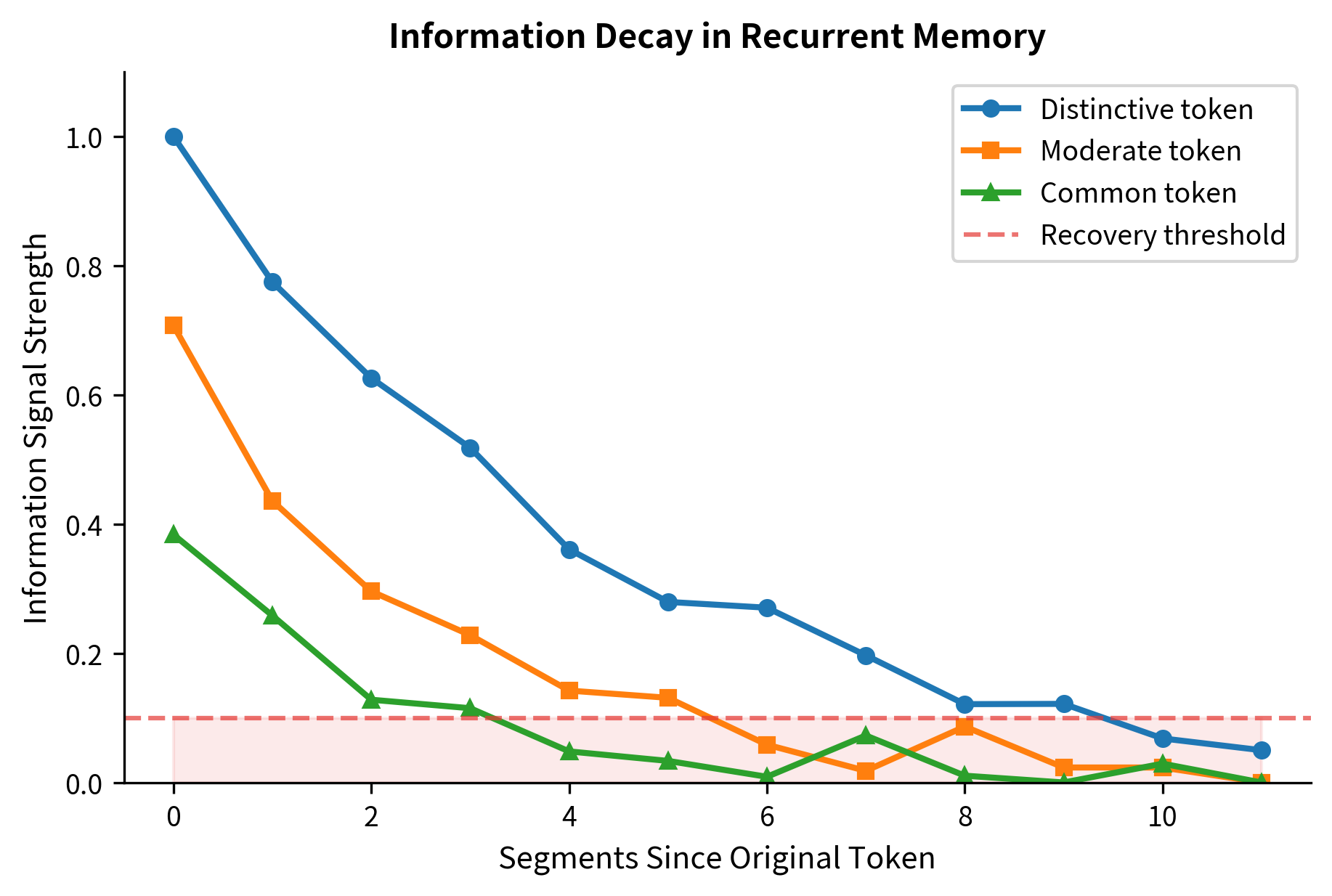
This decay means Transformer-XL works best for gradual, statistical dependencies rather than precise long-range retrieval. Language modeling benefits because most predictions depend on local context with only soft influence from distant text. Tasks requiring exact recall of distant tokens may still fail even with recurrence.

Unidirectional information flow. The recurrence mechanism flows strictly backward in time. Segment 5 can access information from segments 1-4, but segment 2 cannot access information from segment 5. This asymmetry limits bidirectional tasks. For language understanding tasks like question answering where the question appears after the context, the question cannot inform how the context is processed.

Some architectures address this with bidirectional memory or multiple passes, but these increase complexity and computation. The fundamental tradeoff between efficiency and bidirectional context remains.

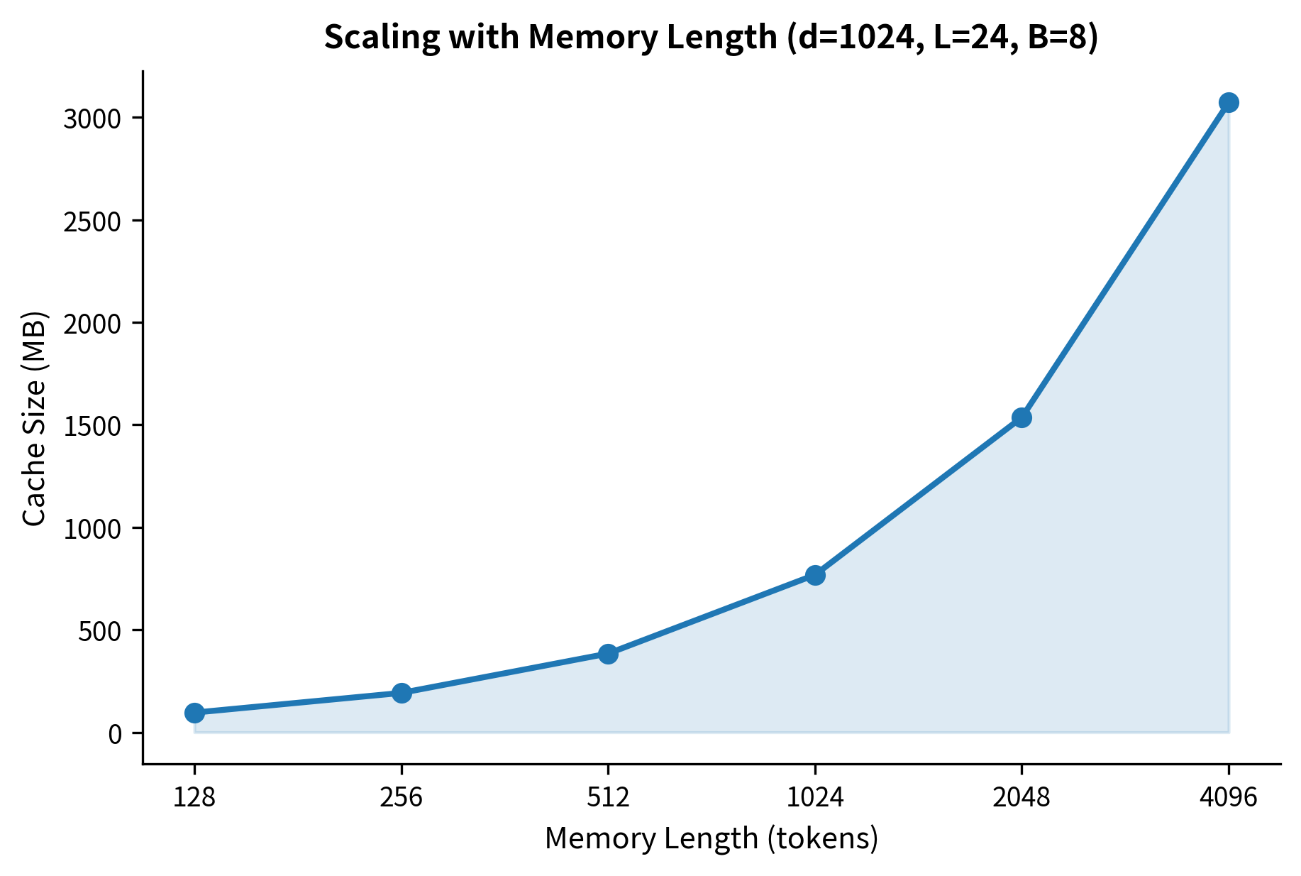
Memory cache management. Storing hidden states for memory consumes GPU memory proportional to:

where:

• $M$: the memory/cache length (number of tokens cached from previous segment)
• $d$: the hidden dimension of the model
• $N_{\text{layers}}$: the number of transformer layers (each layer maintains its own cache)
• $B$: the batch size

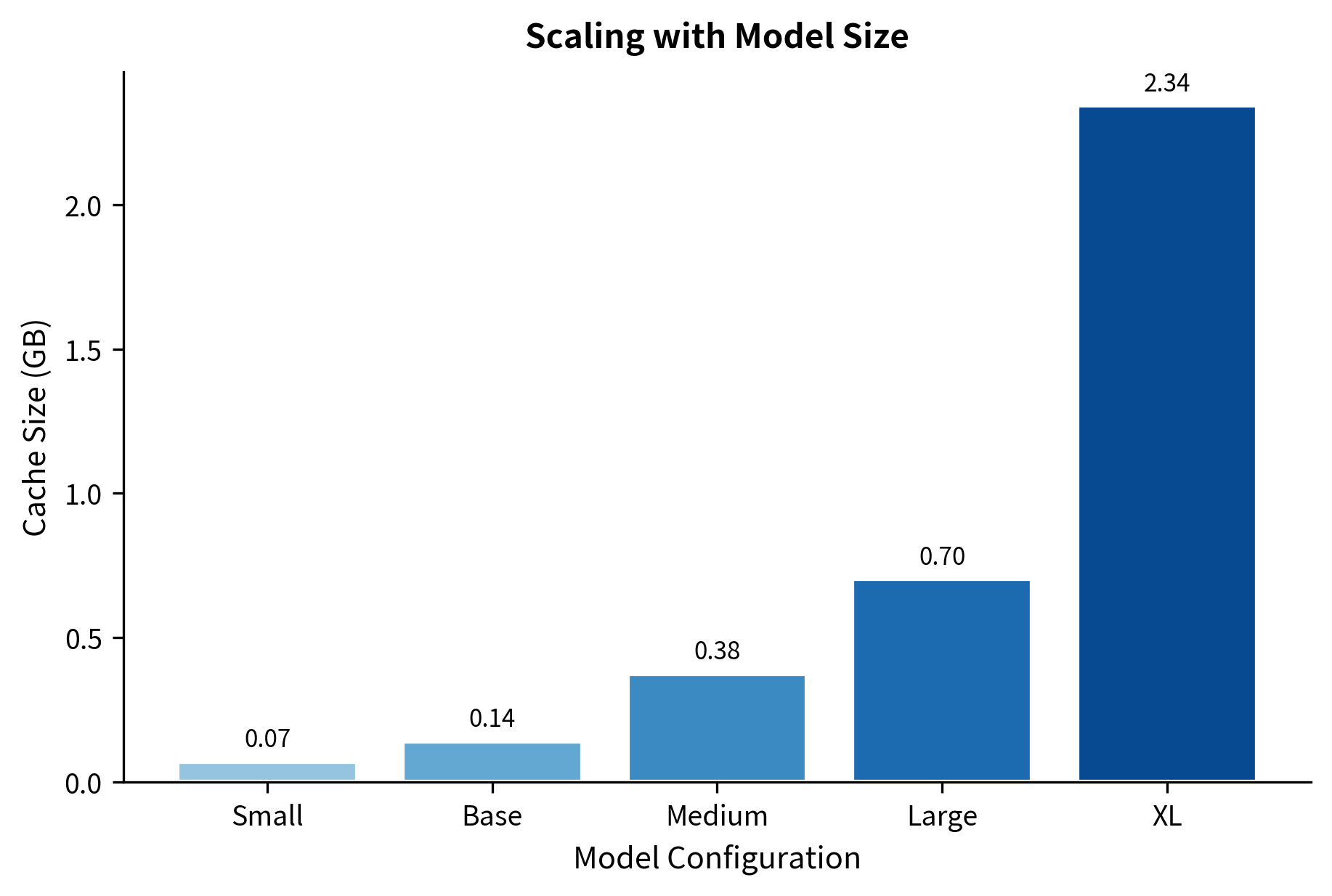
For large models, this becomes substantial. A 24-layer model with hidden dimension 1024 and memory length 512 requires storing over 12 million floats per sample. Batch processing multiplies this further.

The memory requirements grow quickly with model size. A GPT-2 XL scale configuration with 2048-token memory already requires over 2 GB just for the cache, not counting the model weights or activations. This overhead becomes a significant factor when deploying recurrent memory models on resource-constrained hardware.

Training and inference divergence. During training, the memory cache is populated from training data, maintaining realistic statistics. During inference on new text, the cache may be empty at the start, creating a "cold start" problem where initial segments lack the memory context the model learned to expect. Some implementations address this by processing a warmup prefix that isn't used for generation, but this adds latency.

Gradient computation complexity. Although the cached hidden states don't receive gradients (the StopGrad operation), backpropagation still needs to flow through the attention computation over the extended sequence. This slightly increases training complexity compared to pure segment-independent processing, though it's far less expensive than full sequence backpropagation.

Transformer-XL's approach shines in specific scenarios:

• Language modeling on long documents where sequential processing is natural and dependencies decay with distance
• Streaming applications where text arrives incrementally and processing must be online
• Memory-constrained settings where full attention over long sequences is infeasible
• Tasks with local structure where most dependencies are nearby with occasional longer-range influence

The technique is less suitable for:

• Bidirectional understanding tasks requiring simultaneous access to all context
• Exact long-range retrieval where specific facts must be preserved precisely across many segments
• Tasks with unpredictable dependency patterns where important information could appear anywhere

Modern alternatives like FlashAttention and sparse attention patterns have reduced the cost of longer context windows, somewhat diminishing the need for recurrent approaches. However, when truly long sequences must be processed incrementally, segment-level recurrence remains a powerful tool.

This chapter explored Transformer-XL's recurrent memory mechanism, which extends effective context beyond the fixed segment length by caching and reusing hidden states from previous segments.

Context fragmentation, where fixed-length segment processing breaks cross-segment dependencies, fundamentally limits standard transformers. Transformer-XL addresses this by caching the hidden states from the previous segment and concatenating them with the current segment's keys and values. Queries still come only from the current segment, creating an asymmetric attention pattern that enables information flow from past to present.

The recurrence mechanism requires relative position encodings because absolute positions would be ambiguous across segments. Transformer-XL redesigns the attention score computation to depend on the relative distance between query and key positions rather than their absolute locations. This involves replacing the position-dependent terms in attention with learnable global biases and relative position encoding vectors.

The effective context length grows with network depth. Information propagates one segment further back at each layer, so an $N$-layer model has a theoretical reach of $N$ segments beyond the directly attended memory. In practice, information decay limits this reach, but the extension is still substantial.

Key implementation considerations include:

• Memory cache storage scales with memory length, hidden dimension, number of layers, and batch size
• The StopGrad operation prevents backpropagation through cached states, limiting training signal for long-range learning
• Cold start at inference time may require warmup prefixes to populate the cache
• Unidirectional information flow limits applicability to bidirectional tasks

Recurrent memory represents a principled approach to the long-context problem: accept that we cannot attend to everything at once, but ensure that information can flow across the boundaries we impose. While modern advances in attention efficiency have expanded what "at once" can mean, the core insight, that hidden states can carry forward context without explicit attention, remains valuable for streaming and memory-efficient processing of long sequences.

When implementing Transformer-XL or similar recurrent memory mechanisms, the following parameters have the greatest impact on model behavior:

• segment_length: The number of tokens processed in each forward pass. Larger segments capture more local context but increase memory usage quadratically (due to attention). Typical values range from 128 to 512 tokens.

• memory_length: The number of tokens cached from the previous segment. Usually set equal to segment_length, but can be larger to extend context reach at the cost of increased memory and computation.

• num_layers: Deeper networks extend effective context linearly. A 24-layer model can theoretically access 24x more context than a single layer, though information decay limits practical gains.

• d_model: The hidden dimension affects both model capacity and memory requirements. Cache memory scales linearly with this parameter. Common values are 768 (BERT-base) to 1024 (GPT-2).

• max_rel_dist: The maximum relative distance for position encodings. Should be at least segment_length + memory_length to cover all possible query-key distances. Setting this too small causes position information to saturate for distant tokens.

Ready to test your understanding? Take this quick quiz to reinforce what you've learned about Transformer-XL and recurrent memory mechanisms.