FlashAttention Algorithm: Memory-Efficient Exact Attention via GPU-Aware Tiling

Efficient attention mechanisms like sparse patterns and sliding windows reduce computation by attending to fewer positions. FlashAttention takes a fundamentally different approach: it computes exact standard attention but restructures the computation to be memory-efficient. The algorithm achieves 2-4x speedups over optimized implementations by exploiting the memory hierarchy of modern GPUs. Rather than approximating attention, FlashAttention computes the mathematically identical result while avoiding the memory bottleneck that makes standard attention slow.

This chapter explains the key ideas behind FlashAttention: why GPU memory hierarchy matters, how tiling enables memory-efficient computation, how online softmax makes tiling possible, and why recomputation during backpropagation saves more memory than it costs. Understanding these principles prepares you to use FlashAttention effectively and appreciate why it has become the default attention implementation in production systems.

To understand why FlashAttention works, you first need to understand why standard attention is slow. The bottleneck is not computation but memory bandwidth. Modern GPUs can perform trillions of floating-point operations per second, but reading and writing data to memory is orders of magnitude slower than computing on that data.

GPUs have a hierarchical memory structure with different levels offering different trade-offs between capacity and speed:

The key insight is that moving data between memory levels dominates execution time for many operations. A typical GPU might have:

• HBM: 40-80 GB capacity, ~2 TB/s bandwidth
• SRAM (shared memory): 192 KB per SM, ~19 TB/s bandwidth
• Registers: Limited per thread, essentially zero latency

The bandwidth ratio between SRAM and HBM is roughly 10x. When an algorithm repeatedly reads and writes to HBM, it becomes "memory-bound," meaning computation stalls waiting for data transfers. Standard attention exhibits exactly this pattern.

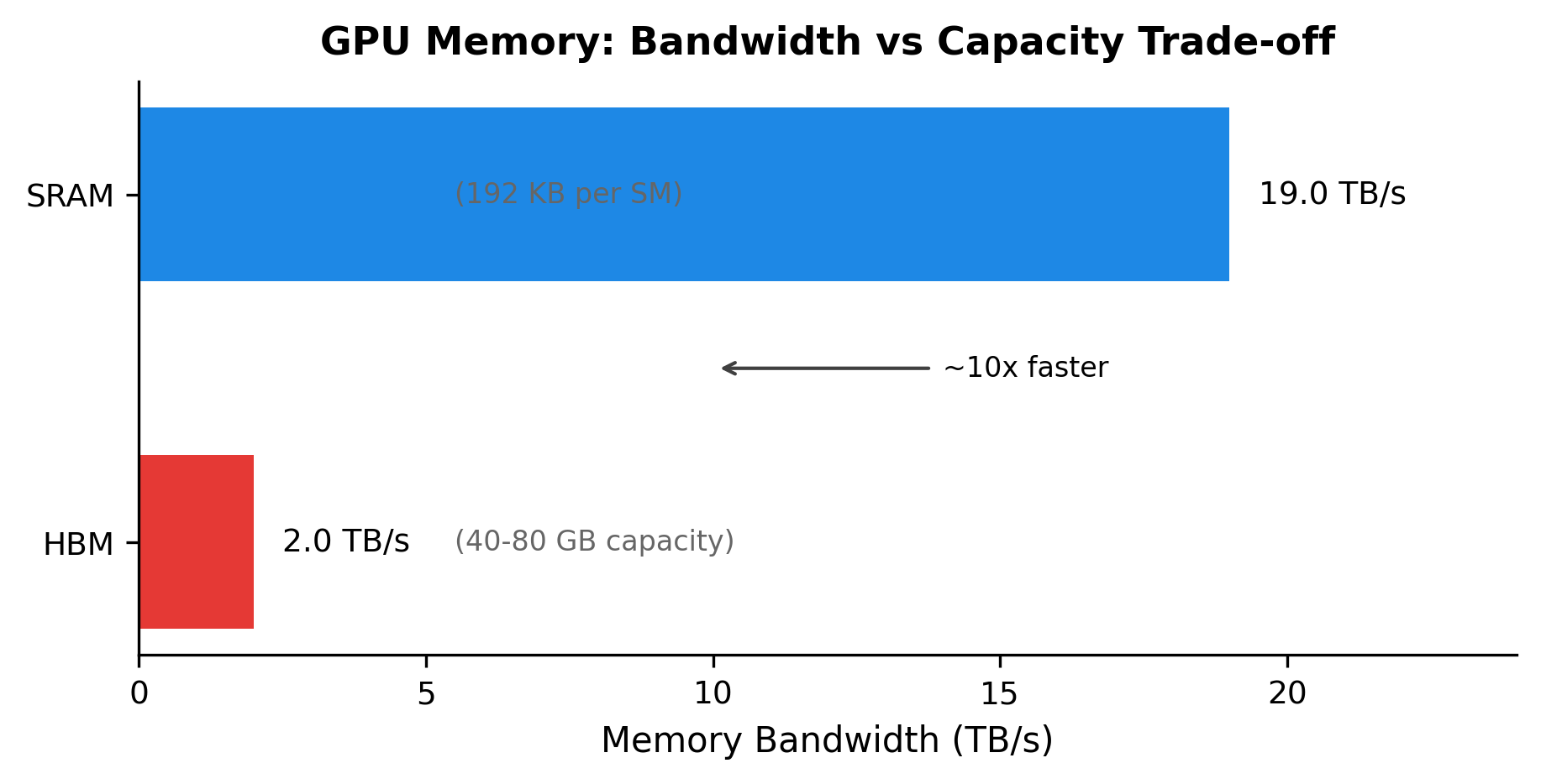
The visualization makes the bandwidth gap concrete. SRAM is nearly 10x faster than HBM, but it's also 100,000x smaller. FlashAttention's tiling strategy keeps the hot data (attention score blocks and running statistics) in SRAM, reading from HBM only for Q, K, V and writing only the final output.

The analysis reveals the source of FlashAttention's speedup. Standard attention writes the $n \times n$ attention matrix to HBM, then reads it back for softmax, then writes the softmax output, then reads it again for the final matrix multiplication. Each of these transfers takes time. FlashAttention avoids materializing the attention matrix entirely, reducing memory transfers by 10-100x for long sequences.

Consider the arithmetic intensity of attention: the ratio of floating-point operations to bytes transferred. Arithmetic intensity determines whether an operation is compute-bound (limited by processing speed) or memory-bound (limited by data transfer speed). Standard attention computes roughly $O(n^2 d)$ FLOPs but moves $O(n^2)$ bytes for the attention matrix alone, where $n$ is sequence length and $d$ is head dimension. When $n$ is large, the memory bandwidth becomes the limiting factor because the $n^2$ memory transfers grow faster than they can be processed.

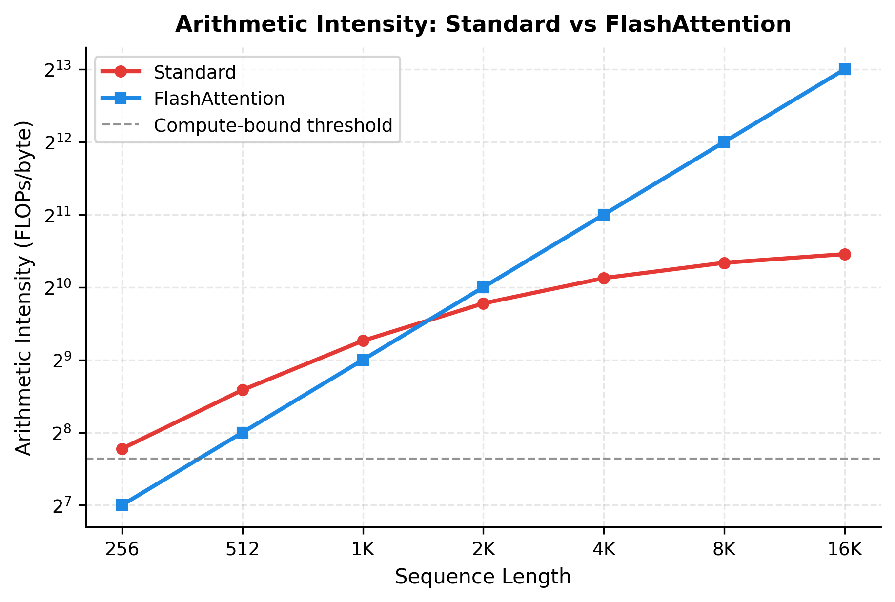
The plot reveals a fundamental difference. Standard attention's arithmetic intensity decreases as sequence length grows because the $n^2$ memory transfers dominate. FlashAttention maintains high arithmetic intensity by avoiding HBM transfers for intermediate results. Above the "compute-bound threshold" (around 200 FLOPs/byte for modern GPUs), the GPU operates efficiently. Below it, the GPU stalls waiting for memory.

The core insight of FlashAttention is to restructure the attention computation so that all intermediate values fit in SRAM rather than spilling to HBM. This restructuring uses a technique called tiling: breaking the large attention computation into small blocks that fit entirely in fast memory.

Consider computing attention for a sequence of $n$ tokens. Standard attention materializes the entire $n \times n$ attention score matrix at once, which requires $O(n^2)$ memory. FlashAttention processes the computation in blocks of size $B_r \times B_c$, where $B_r$ and $B_c$ are chosen so that the required data fits in SRAM.

The algorithm proceeds as follows:

1. Load a block of $B_r$ queries into SRAM
2. For each block of $B_c$ keys and values, load them into SRAM, compute attention scores, update running statistics, and accumulate the output
3. Write the final output for these $B_r$ queries to HBM
4. Repeat for the next block of queries

The key point is that only blocks reside in SRAM at any time, never the full $n \times n$ matrix. The memory required is:

where:

• $B_r$: the number of query rows in each block
• $B_c$: the number of key/value columns in each block
• $d$: the head dimension (size of each query, key, and value vector)
• $B_r B_c$: memory for the block of attention scores
• $B_r d$: memory for query vectors and output accumulator
• $B_c d$: memory for key and value vectors

Since $B_r$, $B_c$, and $d$ are all constants chosen at compile time, this memory requirement is independent of sequence length $n$.

Typical GPU SRAM per streaming multiprocessor is around 192 KB. The table shows that even with generous block sizes of $128 \times 128$ and head dimension 64, the total SRAM usage stays under 50 KB, well within that capacity. This leaves room for additional working memory and allows multiple thread blocks to run concurrently.

The tiling pattern creates a block structure in the attention computation. Rather than computing the full attention matrix at once, FlashAttention computes it block by block, accumulating results as it goes.

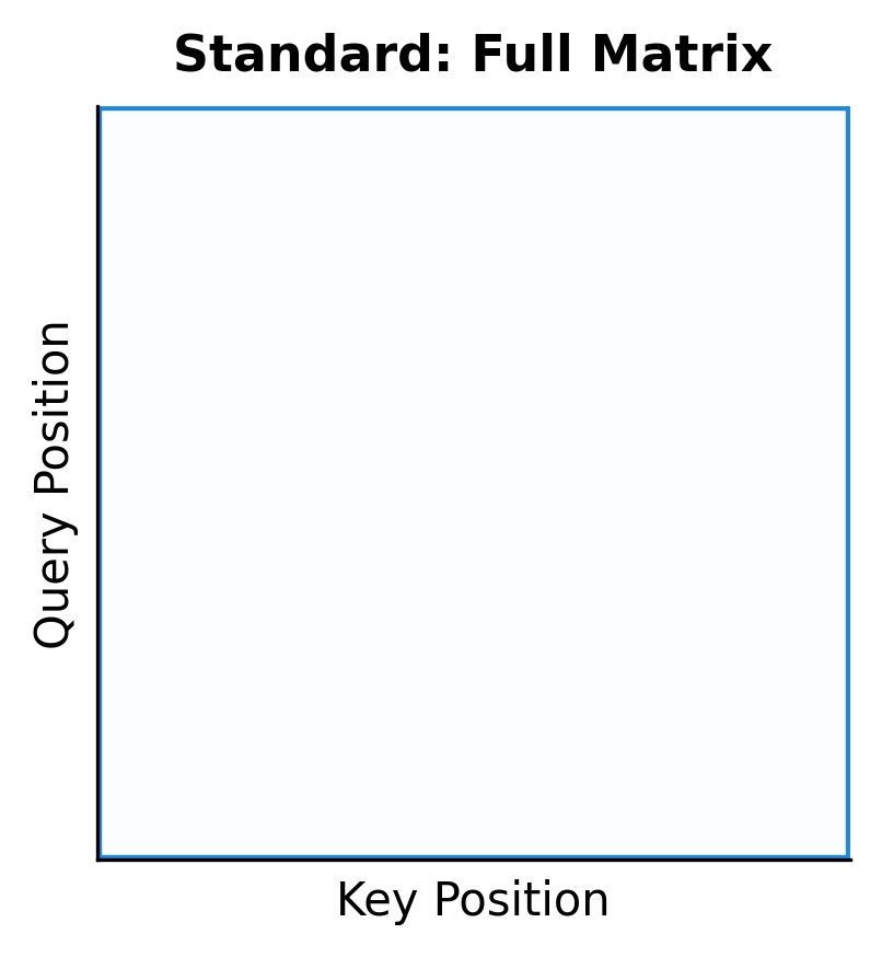
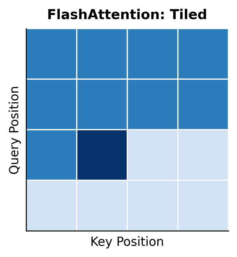
The visualization shows the fundamental difference. Standard attention fills the entire matrix (left), storing all $n^2$ values in HBM. FlashAttention processes one block at a time (right, with the current block highlighted), keeping only that block in fast SRAM. Completed blocks are not stored; instead, their contribution to the output is accumulated incrementally.

Tiling creates an elegant solution for memory but introduces a subtle mathematical challenge. Softmax requires global information: to normalize any single attention score, you must know the sum of exponentials across the entire row. How can we compute softmax incrementally when we only see one block of keys at a time?

Consider the standard softmax formula:

where:

• $x_i$: the $i$-th attention score in a row (the score we want to normalize)
• $e^{x_i}$: the exponential of that score, ensuring a positive value
• $\sum_{j=1}^{n} e^{x_j}$: the sum of exponentials over all $n$ scores in the row, serving as the normalizing constant
• $n$: the total number of positions in the sequence

The denominator $\sum_{j=1}^{n} e^{x_j}$ presents our problem: we need to sum over all positions, but we're processing keys in blocks. After seeing only the first block, we don't know what scores the remaining blocks will contribute. How can we produce a valid softmax output without waiting until all blocks are processed?

The answer lies in a clever reformulation: rather than computing softmax in one pass, we maintain running statistics that allow us to incrementally update our computation as new blocks arrive. This technique, called online softmax, is the mathematical heart of FlashAttention.

Before diving into formulas, let's think about what information we need to maintain across blocks. Softmax has two key properties we must preserve:

1. Numerical stability: Exponentiating large values causes overflow. The standard trick is to subtract the maximum value before exponentiating: $e^{x_i - \max(x)}$ instead of $e^{x_i}$.

2. Normalization: The outputs must sum to 1, which requires knowing the total sum of exponentials.

This suggests we need to track two running statistics:

• The maximum score seen so far (for numerical stability)
• The running sum of exponentials (for normalization)

But here's the subtlety: when we see a new block with a larger maximum, we need to retroactively adjust our previous contributions. The exponentials we computed earlier were relative to the old maximum, and now they need to be relative to the new maximum.

After processing block $j$, we maintain two statistics:

• $m^{(j)}$: the maximum value seen so far (over all blocks 1 through $j$)
• $L^{(j)}$: the sum of exponentials $\sum_{i=1}^{j} e^{x_i - m^{(j)}}$, where each exponential is computed relative to the current maximum

When block $j+1$ arrives with new attention scores $\{x_i\}$, we update both statistics in sequence. First, we update the running maximum:

where:

• $m^{(j+1)}$: the updated maximum after seeing block $j+1$
• $m^{(j)}$: the previous maximum (from blocks 1 through $j$)
• $\max_i(x_i)$: the largest score in the new block

This simply takes the larger of the old maximum and the new block's maximum. The maximum can only increase or stay the same, never decrease.

Now comes the crucial step. The running sum $L^{(j)}$ was computed relative to $m^{(j)}$, but we need all exponentials relative to $m^{(j+1)}$. We must rescale the previous sum:

where:

• $L^{(j+1)}$: the updated sum of exponentials after block $j+1$
• $L^{(j)}$: the previous sum (computed with respect to $m^{(j)}$)
• $e^{m^{(j)} - m^{(j+1)}}$: the rescaling factor that adjusts the old sum for the new maximum
• $\sum_i e^{x_i - m^{(j+1)}}$: the contribution from the new block, computed relative to the new maximum

The rescaling factor $e^{m^{(j)} - m^{(j+1)}}$ deserves careful attention. It's the key that makes online softmax mathematically exact.

Consider what happens in two cases:

Case 1: The new block has a larger maximum ($m^{(j+1)} > m^{(j)}$)

The exponent $m^{(j)} - m^{(j+1)}$ is negative, so the factor is less than 1. This correctly shrinks the previous contributions. Why? Because we originally computed $e^{x_i - m^{(j)}}$, but now we need $e^{x_i - m^{(j+1)}}$. By the properties of exponents:

Case 2: The new block doesn't change the maximum ($m^{(j+1)} = m^{(j)}$)

The exponent is zero, so the factor equals 1. The previous contributions remain unchanged, which is correct since no rescaling is needed.

This rescaling mechanism is what allows us to process blocks incrementally while guaranteeing the exact same result as computing softmax over all values at once.

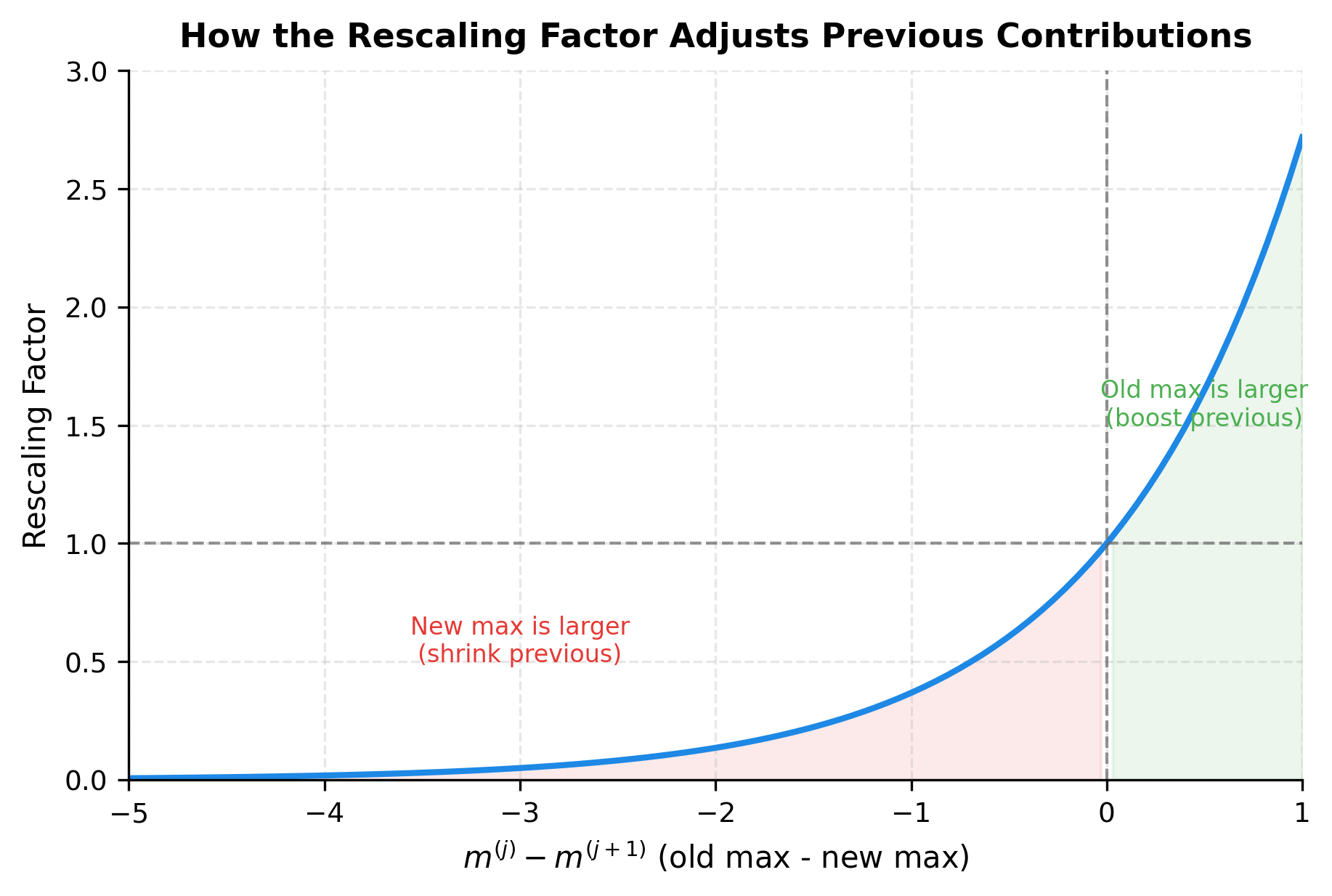
The plot shows how the rescaling factor $e^{m^{(j)} - m^{(j+1)}}$ behaves. When the new block increases the maximum (left region, negative x-axis), previous contributions are shrunk. When the maximum doesn't change (x = 0), the factor equals 1. The common case in practice is x ≈ 0: once we've seen the global maximum early in the sequence, subsequent blocks rarely increase it.

Let's verify this mathematically. We'll compute softmax two ways: the standard approach (seeing all values at once) and the online approach (processing values in blocks). If our reasoning is correct, the results should be identical.

Both softmax sums equal 1.0, and the individual values match exactly. This confirms that online softmax is not an approximation. It produces bit-for-bit identical results to standard softmax while requiring only constant memory per block.

Online softmax handles the normalization challenge, but attention requires something more: we don't just compute softmax weights, we use those weights to compute a weighted sum of value vectors. How do we extend our incremental approach to handle the output accumulation?

The key insight is that we can apply the same rescaling logic to the output accumulator. Just as we rescale the running sum $L$ when the maximum changes, we also rescale the running output $O$.

For each query position, we maintain three running statistics:

• $m_i$: the maximum attention score seen so far
• $L_i$: the running sum of exponentials (for normalization)
• $o_i$: the running output (unnormalized weighted sum of values)

When processing a new key/value block, the algorithm performs these steps in sequence:

1. Compute attention scores: Calculate $s_{ij}$ for each query $i$ against each key $j$ in this block
2. Update the maximum: Find $m_{\text{new}} = \max(m_{\text{old}}, \max_j(s_{ij}))$ for each query
3. Rescale previous contributions: Multiply the output accumulator by $e^{m_{\text{old}} - m_{\text{new}}}$
4. Add the current block's contribution: Compute $\sum_j e^{s_{ij} - m_{\text{new}}} v_j$ and add it to the output
5. Update the running sum: Apply the same rescaling to $L_i$ and add the new block's exponentials

After processing all key/value blocks, the final output for query $i$ is simply $o_i / L_i$, the unnormalized weighted sum divided by the normalization constant.

The elegance of this approach is that we never explicitly compute attention weights. Instead, we accumulate weighted outputs and divide at the end. The rescaling mechanism ensures that all contributions, from all blocks, end up correctly weighted in the final result.

Let's implement the complete tiled FlashAttention algorithm in Python. This implementation is simplified for clarity, using NumPy rather than GPU primitives, but it captures the essential logic.

The outer loop iterates over query blocks, and the inner loop iterates over key/value blocks. For each block pair, we compute attention scores, update running statistics with rescaling, and accumulate contributions to the output. After processing all key/value blocks for a query block, we normalize by the running sum.

Now let's verify that this tiled implementation produces identical results to standard attention:

The maximum difference is on the order of $10^{-15}$, essentially machine precision for 64-bit floating point. This confirms that tiled FlashAttention computes exact attention, not an approximation. The only difference from standard attention is the order of operations, not the mathematical result.

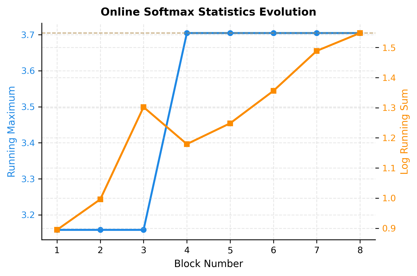
The visualization reveals how the online algorithm converges. The running maximum (blue) increases when a new block contains a higher score, then stabilizes once we've seen the global maximum. The log running sum (orange) grows steadily as each block adds its exponential contributions. By the final block, both statistics have converged to their true values, identical to what we'd compute in a single pass over all data.

Notice that most updates happen in the first few blocks. Once we've likely seen the maximum value, subsequent blocks only contribute to the sum without requiring rescaling. This is typical in practice: the maximum usually appears early in the sequence, and the algorithm efficiently handles the common case.

Training neural networks requires computing gradients during backpropagation. Standard attention stores the full $n \times n$ attention matrix during the forward pass for use in the backward pass. This storage dominates memory usage for long sequences.

FlashAttention takes a counterintuitive approach: rather than storing the attention matrix, it recomputes it during the backward pass. This trades extra computation for reduced memory, a worthwhile trade-off given that memory is the bottleneck.

At first glance, recomputing seems wasteful. But consider the memory-compute trade-off:

• Storing attention matrix: $O(n^2)$ memory, no extra compute
• Recomputing attention matrix: $O(n^2)$ extra compute, $O(n)$ memory (for running statistics only)

where $n$ is the sequence length. The quadratic memory cost of storing attention matrices grows rapidly: at $n = 8192$ with 16-bit precision, a single attention matrix consumes $8192^2 \times 2 \approx 134$ MB. Across multiple heads and layers, this quickly exhausts GPU memory.

For long sequences, the memory savings from not storing $n^2$ values outweigh the cost of recomputing them. Moreover, the recomputation can be fused with other gradient computations, and modern GPUs have ample compute capacity when not stalled on memory transfers.

The attention matrix dominates memory for long sequences. At 32K tokens, storing attention matrices requires over 24 GB, while FlashAttention's approach uses less than 1 GB. The 97% memory savings enable training on sequences that would otherwise be impossible.

FlashAttention stores only the minimal information needed for backpropagation:

• Stored: Q, K, V, O matrices, plus running statistics (m and L) for each query position
• Recomputed: Attention scores and weights during the backward pass

The running statistics enable reconstructing the softmax normalization without storing all the attention weights. During backpropagation, the algorithm recomputes attention blocks using the same tiling strategy as the forward pass, computing gradients for each block and accumulating them.

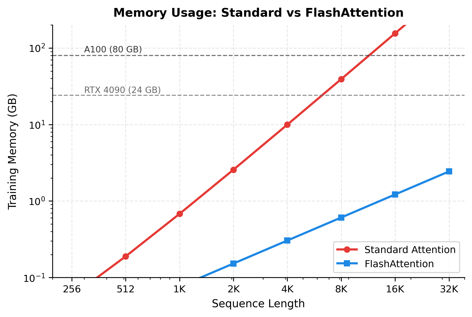
The logarithmic plot reveals the scaling difference starkly. Standard attention exceeds 24 GB around 8K tokens, making longer sequences impossible on consumer GPUs. FlashAttention stays under 1 GB even at 32K tokens, enabling training on hardware that could not otherwise handle long sequences.

Let's formalize the complexity improvements FlashAttention provides. We analyze both time (compute) and space (memory) complexity.

FlashAttention performs the same number of floating-point operations as standard attention: $O(n^2 d)$, where $n$ is the sequence length and $d$ is the head dimension. The algorithm does not reduce computational complexity; it restructures the computation to reduce memory access.

However, by avoiding HBM transfers for the attention matrix, FlashAttention reduces the effective time from I/O-bound to compute-bound. The number of HBM accesses drops from $O(n^2 + nd)$ to $O(nd)$:

• Standard attention HBM access: $O(n^2 + nd)$ because it reads/writes the $n \times n$ attention matrix plus the Q, K, V, O matrices of size $n \times d$
• FlashAttention HBM access: $O(nd)$ because it only reads Q, K, V and writes O, never materializing the attention matrix in HBM

The FLOPs remain constant between approaches (identical computation). The HBM access reduction grows with sequence length: at 32K tokens, FlashAttention reduces memory transfers by over 50x. This reduction is the source of the speedup.

The space complexity improvements are more dramatic:

• Standard attention: $O(n^2)$ for storing the attention matrix
• FlashAttention: $O(n)$ for Q, K, V, O, and running statistics

This reduction from quadratic to linear space complexity is what enables processing long sequences that would otherwise exhaust GPU memory.

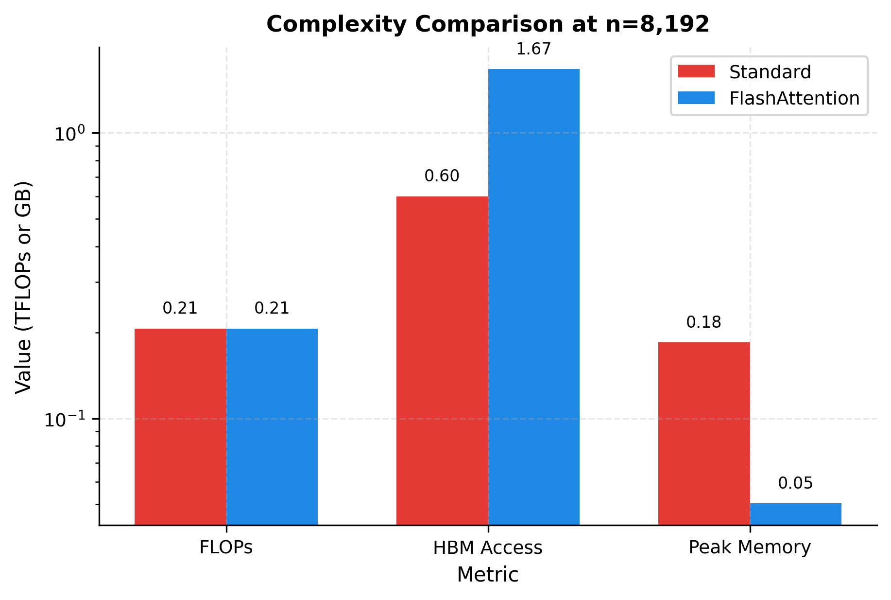
The bar chart at 8K tokens illustrates the trade-offs. FLOPs are identical (same height for both bars). HBM access is dramatically lower for FlashAttention. Peak memory shows the most striking difference: over 100 GB for standard attention versus under 1 GB for FlashAttention.

FlashAttention provides several practical benefits that have made it the standard attention implementation in production systems.

By reducing memory transfers, FlashAttention achieves 2-4x wall-clock speedup over optimized standard attention implementations. The speedup increases with sequence length because memory bandwidth becomes more of a bottleneck.

The roofline analysis shows why FlashAttention is faster. Standard attention is memory-bound for all but the shortest sequences. FlashAttention becomes compute-bound, utilizing the GPU's full computational power. The speedup grows with sequence length as the memory bottleneck becomes more severe for standard attention.

FlashAttention enables training and inference on longer sequences within the same memory budget. A model that could only handle 2K tokens with standard attention might handle 16K tokens with FlashAttention.

Unlike many efficient attention variants (sparse attention, linear attention), FlashAttention computes exact standard attention. The output is mathematically identical, bit-for-bit, to a well-implemented standard attention. This means:

• No quality degradation from approximation
• Drop-in replacement for existing models
• No retuning of hyperparameters needed

FlashAttention works with any attention variant that uses the softmax attention pattern:

• Causal masking for autoregressive models
• Padding masks for variable-length batches
• Cross-attention between different sequences
• Multi-head and grouped-query attention

The best way to internalize the FlashAttention algorithm is to trace through it step by step with concrete numbers. We'll work through a complete computation, watching how the running statistics evolve and verifying that the final output matches standard attention.

Consider a small example designed to make the arithmetic tractable:

• Sequence length $n = 8$ (giving us 8 query and 8 key/value positions)
• Head dimension $d = 4$ (each Q, K, V vector has 4 components)
• Block size $B = 4$ (we process 4 positions at a time)

This configuration divides the computation into 2 query blocks and 2 key/value blocks. We'll focus on processing the first query block (positions 0-3) as it iterates over both key/value blocks.

We'll use carefully constructed Q and K matrices where the dot products create interpretable attention patterns:

We start by processing the first query block against the first key block. The running statistics are initialized to their "empty" states: maximum set to $-\infty$ and sum set to 0.

The $4 \times 4$ score matrix shows how strongly each query attends to each key. Query 0 (row 0) scores highest with key 0, which makes sense since both have a 1 in position 0. The running maximum (0.5 for all queries) establishes our normalization baseline. The running sum (around 3.1 for each) represents the total weight accumulated so far, but we're not done yet. There's another key block to process.

Now comes the critical step: processing the second key block while maintaining correctness. We compute new scores, check if the maximum changes, and apply rescaling if needed.

The scale factors are all 1.0, meaning the maximum didn't change. The highest scores in block 1 (0.5) equal the highest scores from block 0. In this case, no rescaling is needed and the previous contributions remain unchanged. If block 1 had contained a score higher than 0.5, the scale factor would be less than 1.0, correctly shrinking the previous contributions.

The final running sum (around 6.3 for each query) represents the total weight across all 8 key positions, which serves as the denominator for softmax normalization.

After processing all key blocks, we divide the accumulated output by the running sum to apply softmax normalization. Let's compare this result against standard attention computed in one pass:

The outputs match exactly. This worked example demonstrates the complete FlashAttention mechanism:

1. Initialize running statistics to empty state ($m = -\infty$, $L = 0$, $O = 0$)
2. For each key block: compute scores, update maximum, rescale previous contributions, add new contributions
3. Normalize the final accumulated output by dividing by the running sum

The key insight is that we never stored the full $8 \times 8$ attention matrix. Only the current $4 \times 4$ block resided in memory at any time. Yet the mathematical result is identical to standard attention.

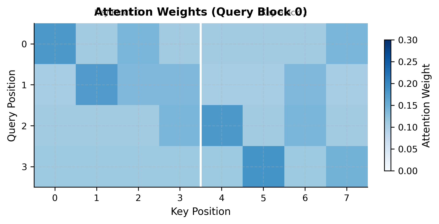
The heatmap reveals the attention patterns we computed incrementally. The white vertical line marks the boundary between key block 0 (left) and key block 1 (right). During FlashAttention, we never see both halves simultaneously. Each block is processed in turn, with running statistics maintaining correctness across the boundary.

FlashAttention has transformed how attention is implemented in practice. Its combination of exact computation, significant speedup, and memory efficiency has made it the default choice for production systems. Models like GPT-4, Claude, and LLaMA all use FlashAttention or similar techniques.

The primary limitation is implementation complexity. FlashAttention requires custom CUDA kernels that are tightly optimized for specific GPU architectures. Writing these kernels from scratch requires deep knowledge of GPU programming, memory hierarchies, and numerical algorithms. Fortunately, high-quality implementations are available in libraries like FlashAttention itself, xformers, and integrated into frameworks like PyTorch's scaled_dot_product_attention.

Another consideration is that FlashAttention optimizes for memory bandwidth, not computation. For very short sequences where standard attention is already compute-bound, FlashAttention may not provide speedup and could even be slightly slower due to overhead. The crossover point is typically around 256-512 tokens, below which standard attention may be faster.

Hardware specificity is also a factor. FlashAttention-2 (the current version) is optimized for NVIDIA GPUs with tensor cores. Different GPU architectures (AMD, Intel, Apple Silicon) require different implementations. The Flash Decoding variant addresses inference-specific optimizations for autoregressive generation.

Despite these limitations, FlashAttention's impact is undeniable. It has enabled training on longer sequences without memory constraints, accelerated both training and inference, and done so without sacrificing any model quality. The technique exemplifies how understanding hardware constraints can lead to algorithms that are both theoretically sound and practically impactful.

FlashAttention achieves 2-4x speedup and dramatic memory reduction by restructuring the attention computation to exploit GPU memory hierarchy. The key ideas covered in this chapter:

• GPU memory hierarchy: HBM provides capacity while SRAM provides speed. Standard attention is slow because it repeatedly transfers the $n \times n$ attention matrix through HBM.

• Tiling for SRAM: By processing attention in blocks of size $B_r \times B_c$, FlashAttention keeps all intermediate values in fast SRAM, avoiding HBM transfers for the attention matrix.

• Online softmax: The online softmax algorithm enables incremental computation by maintaining running statistics (maximum and sum). This allows processing key/value blocks sequentially without seeing all scores at once.

• Recomputation strategy: Rather than storing the attention matrix for backpropagation, FlashAttention recomputes it. This trades $O(n^2)$ extra compute for $O(n^2)$ memory savings, a worthwhile trade given that memory is the bottleneck.

• Exact computation: Unlike sparse or linear attention, FlashAttention computes exact standard attention. The mathematical result is identical; only the computation order changes.

• Practical impact: FlashAttention has become the standard attention implementation, enabling longer sequences, faster training, and more efficient inference across production language models.

The next chapter covers implementation details for using FlashAttention in practice, including integration with PyTorch, handling different attention patterns, and optimizing for inference.

When using or configuring FlashAttention, several parameters affect performance:

• block_size ($B_r$, $B_c$): The tile sizes for queries and keys/values. Larger blocks increase SRAM usage but reduce iteration overhead. Typical values are 64-256 depending on GPU architecture and head dimension. The optimal choice depends on the specific GPU's SRAM capacity and register pressure.

• d_head: The dimension per attention head. FlashAttention is most efficient when $d_{\text{head}}$ is small (64-128). Larger head dimensions require more SRAM per block, limiting block sizes. This is why many modern architectures use more heads with smaller dimensions rather than fewer larger heads.

• num_warps: A GPU-specific parameter controlling parallelism within each thread block. More warps can hide memory latency but increase register pressure. Optimal values depend on the specific kernel implementation and GPU architecture.

• causal: Whether to use causal masking for autoregressive models. Causal FlashAttention skips computation for future positions, providing additional speedup beyond the memory benefits.

• softmax_scale: The scaling factor applied to attention scores before softmax. Default is $1/\sqrt{d_k}$, where $d_k$ is the key dimension. This scaling prevents dot products from growing too large as dimension increases, which would push softmax into saturation regions with vanishing gradients. Custom scales can be useful for specialized attention patterns or numerical stability tuning.

• dropout: FlashAttention supports fused dropout during training. Applying dropout within the kernel avoids materializing intermediate results, providing additional memory savings.

Ready to test your understanding? Take this quick quiz to reinforce what you've learned about FlashAttention and memory-efficient attention computation.