

Learn how QKV projections enable transformers to learn flexible attention patterns through specialized query, key, and value representations.

This article is part of the free-to-read Language AI Handbook
Choose your expertise level to adjust how many terms are explained. Beginners see more tooltips, experts see fewer to maintain reading flow. Hover over underlined terms for instant definitions.
Query, Key, Value
In the previous chapter, we implemented self-attention using raw embeddings: each token's embedding served directly as the basis for computing similarities and aggregating context. This approach works, but it has a fundamental limitation. When a token computes dot products with other tokens using its own embedding, it's asking: "Which tokens are similar to me?" But similarity isn't the same as relevance. A pronoun like "it" isn't similar to "cat" in embedding space, yet "cat" is highly relevant for understanding what "it" refers to.
The solution is to give tokens different representations for different roles. When a token is looking for context (querying), it should express what information it needs. When a token is being looked at (acting as a key), it should advertise what information it offers. And when a token contributes to another token's representation (providing a value), it should supply the actual content to be aggregated. This separation of concerns is the Query, Key, Value (QKV) framework.
The Database Lookup Analogy
The QKV mechanism mirrors how databases retrieve information. Consider a library catalog: you search with a query (perhaps "books about neural networks"), the system compares your query against keys (book metadata, titles, descriptions), and returns values (the actual book content or references). The query expresses what you want, keys describe what's available, and values provide the substance.
In self-attention, each token is projected into three different representations: a query (what information am I looking for?), a key (what information do I contain?), and a value (what information should I contribute?). Attention weights are computed by matching queries to keys, then used to aggregate values.
This analogy clarifies why raw embedding similarity falls short. In a database, your search query isn't compared directly against the books themselves; it's compared against structured metadata designed to facilitate matching. Similarly, in self-attention, we don't want tokens to match based on their raw meanings. We want them to match based on learned patterns that capture functional relationships: subjects matching predicates, pronouns matching antecedents, modifiers matching their targets.
The QKV Mechanism: From Intuition to Formula
Now that we understand why we need separate representations for querying, being queried, and contributing content, let's build up the mathematical machinery that makes this work. We'll develop each component step by step, showing how the formulas directly address the challenge of learning flexible attention patterns.
The journey from intuition to formula follows a natural progression:
- Project tokens into specialized query, key, and value spaces
- Measure compatibility between queries and keys using dot products
- Scale the scores to prevent numerical instability
- Aggregate values according to the attention weights
Each step solves a specific problem that arises from the previous one. By the end, you'll see how these pieces combine into a single elegant formula that powers modern transformers.
Step 1: Projecting Into Specialized Spaces
The core insight is simple: if we want tokens to play different roles, we should give them different representations for each role. We accomplish this through learned linear projections, three separate transformations that map each token's embedding into query, key, and value spaces.
Why three separate projections? Consider what happens when a pronoun like "it" needs to find its antecedent. The pronoun's embedding encodes "third-person singular neuter pronoun," but that's not what it should search for. It should search for "noun phrase that could be referred to." Meanwhile, a noun like "cat" shouldn't advertise "I'm a cat" but rather "I'm a noun phrase available for reference." And when "cat" contributes information, it should provide its semantic content (the concept of a cat), not its grammatical role.
These are three fundamentally different jobs:
- Querying: What information am I looking for?
- Being queried: What information do I have to offer?
- Contributing: What content should I transmit?
A single embedding can't optimally serve all three purposes. So we learn three different transformations, each specialized for its role.
Given an input embedding for a single token, we compute:
where:
- : the input embedding vector (a row vector with dimensions)
- : the resulting query vector, expressing what this token is looking for
- : the resulting key vector, advertising what this token contains
- : the resulting value vector, carrying the content to be aggregated
- : the query projection matrix (learned during training)
- : the key projection matrix (learned during training)
- : the value projection matrix (learned during training)
- : the input embedding dimension
- : the dimension of queries and keys (must match for dot product compatibility)
- : the dimension of values (can differ from )
Each projection is a matrix multiplication, a linear transformation where each output dimension is a weighted combination of input dimensions. The crucial point is that these weights are learned during training. The model doesn't know in advance which embedding features matter for querying versus being queried versus contributing content. Instead, gradient descent discovers these patterns from data:
- learns which combinations of embedding features make effective queries (what patterns indicate "I need information about X")
- learns which combinations make effective keys (what patterns indicate "I have information about X")
- learns which content is worth transmitting when attention flows
This learning happens implicitly through the training objective. If attending from a verb to its subject improves next-word prediction, the projection matrices gradually adjust to make verb queries match subject keys.
Scaling to sequences. For a complete sequence of tokens, we stack all embeddings into a matrix (where each row is one token) and project all tokens simultaneously:
The resulting matrices have shapes , , and . Row of each matrix is the query, key, or value vector for token .
Why might these projections learn different things? Consider an embedding that encodes both syntactic information (part of speech, grammatical role) and semantic information (meaning, topic). The query projection might learn to emphasize syntactic features, helping verbs find their subjects by grammatical role rather than semantic similarity. Meanwhile, the value projection might preserve semantic content, so that when attention flows, it transfers meaning rather than grammatical markers.
The separation between keys and values is particularly powerful. A word's key determines which queries it matches (what attention it receives), while its value determines what information it contributes. This decoupling means a word can attract attention for one reason (syntactic role) while contributing entirely different information (semantic content).
Step 2: Measuring Compatibility with Dot Products
With queries and keys in hand, we face the next challenge: how do we measure whether a query matches a key? We need a scoring function that takes two vectors and returns a single number indicating compatibility. Higher numbers should mean better matches.
Several options exist, including additive attention, multiplicative attention, and others, but the dot product has become the standard choice for its simplicity and efficiency. The geometric interpretation is intuitive:
- Vectors pointing in the same direction → large positive dot product (strong match)
- Orthogonal vectors → zero dot product (no relationship)
- Vectors pointing in opposite directions → negative dot product (poor match)
This gives us exactly the ranking behavior we want: the most compatible keys get the highest scores, and training can learn arbitrary matching patterns by adjusting the projection matrices.
For positions and , the compatibility score is:
where:
- : the raw attention score measuring how well position 's query matches position 's key
- : the query vector for position
- : the key vector for position
- , : the -th components of these vectors
- : the dimension of query and key vectors (must match for the dot product to be defined)
The beauty of the dot product is that it's differentiable, fast to compute, and captures alignment in learned representation space. Because and come from learned projections, the model can discover arbitrary matching patterns during training.
To compute all scores at once (every query against every key), we use matrix multiplication:
where:
- : the score matrix containing all pairwise attention scores
- : the query matrix (row is the query for position )
- : the transposed key matrix (column is the key for position )
Entry is the dot product of row of with column of , which equals . This single matrix multiplication gives us all pairwise scores in one highly optimized operation, a key reason why attention scales well on modern hardware.
The power of learned projections. This is where QKV attention differs fundamentally from raw embedding similarity. In the previous chapter, tokens matched based on how similar their embeddings were, a fixed computation that couldn't adapt to context. Now they match based on how well their learned projections align.
Consider the implications: a verb's query can learn to match the key of a noun playing the subject role, even if "run" and "dog" have very different embeddings. The word "it" can learn a query that matches noun phrase keys, even though pronouns and nouns occupy different regions of embedding space. The projections transform the matching problem from "what words are similar?" to "what words are relevant?", and relevance is learned from data.
Step 3: The Scaling Problem and Its Solution
We have scores, but there's a subtle problem lurking in the mathematics. As the dimension grows, dot products tend to become larger in magnitude, not because the vectors are more aligned, but simply because we're summing more terms. This creates numerical instability that can derail training. To understand why and how we fix it, let's work through the statistics step by step.
Setting up the problem. Assume each component of and has zero mean and unit variance (a reasonable assumption for normalized embeddings). We want to understand how the variance of the dot product depends on dimension.
Step 1: Write the dot product as a sum. The dot product is:
where:
- : the -th component of the query vector
- : the -th component of the key vector
- : the dimension of both vectors
Step 2: Compute variance of each term. Each product is the product of two independent random variables with zero mean and unit variance. For independent random variables and with and :
So each term has variance 1.
Step 3: Sum the variances. For independent random variables, the variance of a sum equals the sum of variances:
Conclusion. The dot product has variance , so its standard deviation is . At (common in practice), scores have standard deviation 8. At , it's about 22.6. This growth in magnitude isn't a feature; it's a bug that we need to fix.
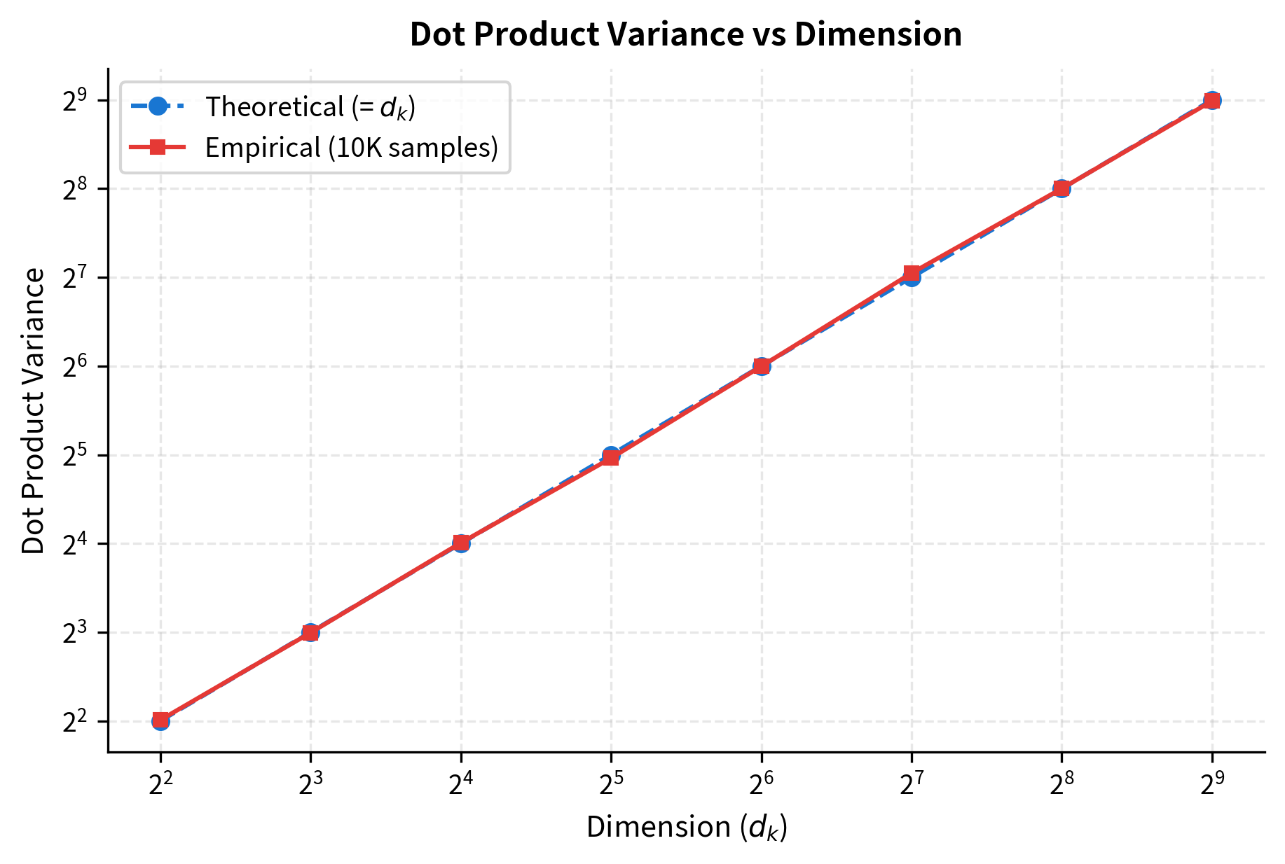
The plot confirms our theoretical prediction: variance grows linearly with dimension. The empirical measurements (red squares) lie almost perfectly on the theoretical line (blue circles), validating our statistical analysis.
Why does this matter? The problem becomes clear when we consider what happens next: we apply softmax to convert scores into probability-like attention weights.
The softmax function converts a vector of real numbers into a probability distribution. For a vector of scores , softmax computes:
where:
- : the -th score (the raw attention score for position )
- : the exponential of , ensuring all values become positive
- : the sum of exponentials across all positions, serving as a normalizing constant
- : the number of positions (sequence length)
The exponential function amplifies differences between inputs: larger scores get exponentially larger outputs. When one score is much larger than others, softmax assigns nearly all probability mass to that element. The attention becomes "hard," focusing on essentially one position while ignoring all others.
More critically, this creates gradient problems. In the softmax function, elements with very low probability receive vanishingly small gradients. If attention is sharply focused due to large score magnitudes, the model struggles to learn that other positions might also be relevant. Training becomes slow and unstable.
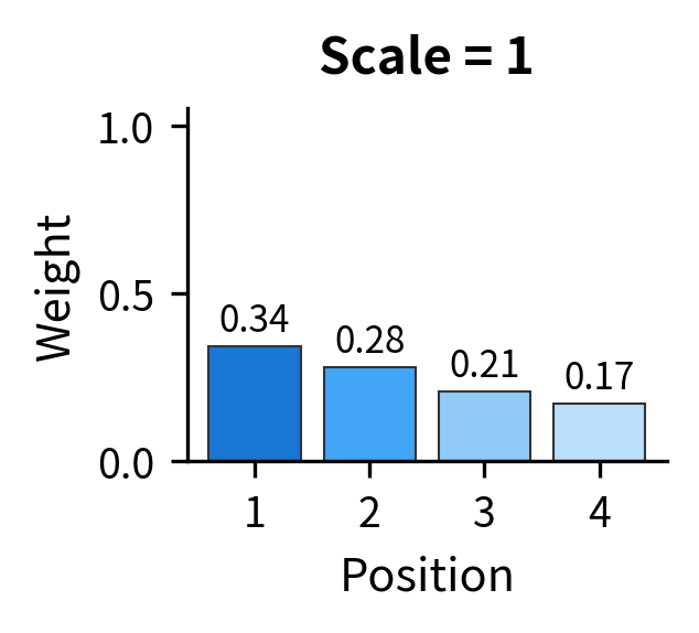
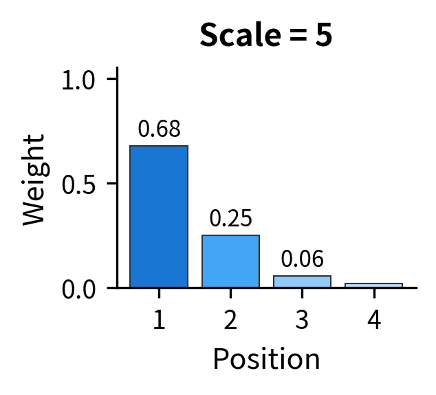
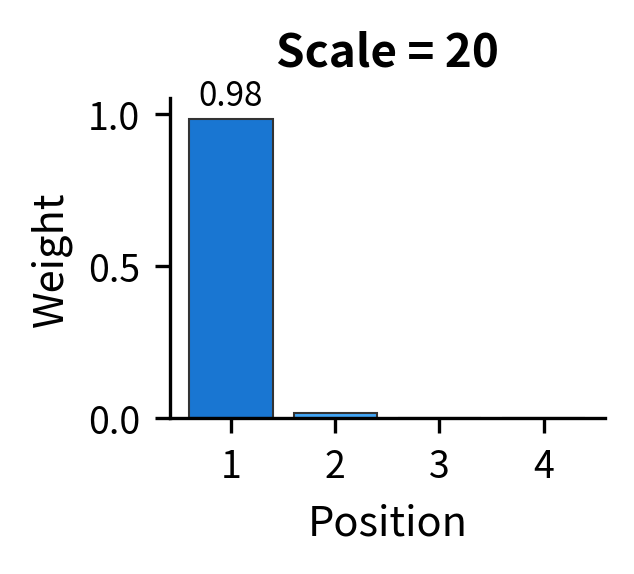
The visualization makes the problem viscerally clear. All three plots use scores with the same relative differences, where position 1's score is always 25% higher than position 2's, and so on. But scaling up the magnitudes completely changes the output distribution. In the rightmost plot, position 1 receives 99.9% of the weight, and the model can barely learn to attend elsewhere.
The elegant solution. Since the problem is that score variance grows with , we fix it by dividing scores by . This simple scaling operation normalizes the variance back to approximately 1, regardless of dimension:
- Original variance:
- After scaling by : variance becomes
The result is the complete scaled dot-product attention formula:
where:
- : the query matrix, with row containing the query vector for position
- : the key matrix, with row containing the key vector for position
- : the value matrix, with row containing the value vector for position
- : the raw score matrix, where entry is the dot product
- : the scaling factor that stabilizes score magnitudes
- : applied row-wise, converts each row of scaled scores into a probability distribution (attention weights)
- : the sequence length (number of tokens)
- : the query/key dimension
- : the value dimension (determines the output dimension)
The formula works in three stages. First, computes all pairwise query-key dot products. Second, dividing by and applying softmax converts these scores into attention weights. Third, multiplying by aggregates value vectors according to these weights, producing context-enriched output representations.
After scaling, scores have controlled variance regardless of , and softmax operates in a regime where gradients flow to all positions.
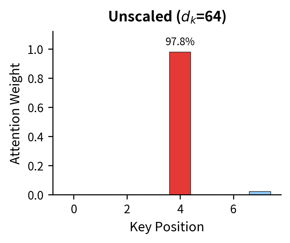
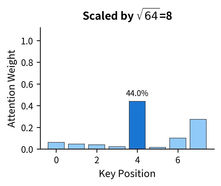
The side-by-side comparison demonstrates scaling's importance. Without it (left), attention collapses to a near-hard distribution where one position dominates. With scaling (right), the model retains flexibility to attend broadly. Crucially, gradients flow to all positions during training, allowing the model to learn nuanced attention patterns.
Let's verify that the dimensions work out correctly by tracing through a concrete example:
The shapes confirm our understanding: input embeddings flow through projections to create Q, K, and V. The attention weight matrix is always because we compute all pairwise interactions. The output has the same sequence length as the input but takes on the value dimension . In practice, is often chosen to equal and the original embedding dimension, enabling residual connections.
Step 4: Aggregating Values
We've now computed attention weights, a probability distribution over positions for each query. But weights alone don't produce useful outputs. The final step uses these weights to aggregate value vectors, producing new representations enriched with contextual information.
This is where the separation of keys and values proves its worth. Keys determined which positions receive attention (through query-key matching). Values determine what content actually flows. A word might attract attention because of its syntactic role (captured in its key) while contributing semantic information (carried in its value).
For position , the output is a weighted sum of all value vectors:
where:
- : the output vector for position , now enriched with contextual information
- : the attention weight from position to position , indicating how much position attends to position
- : the value vector at position , carrying the content that can be transferred
- : the sequence length (total number of positions)
- : the value dimension
The attention weights come from applying softmax to the scaled scores, so they satisfy for each position . This constraint ensures the output is a proper weighted average.
Geometrically, this weighted average has an elegant interpretation. Position 's output is a blend of all value vectors, with weights determined by query-key compatibility. Positions with keys that matched 's query (high ) contribute more; positions with mismatched keys (low ) contribute less. Because the weights sum to 1, the output lies within the convex hull of the value vectors, a point "inside" the space spanned by all possible values.
The information flow paradigm. Self-attention can be understood as a message-passing system. Each position broadcasts its value vector, and each position receives a custom blend of all broadcasts, with the blend weights determined by query-key compatibility. Unlike recurrent networks that pass information sequentially, or convolutional networks that only see local neighborhoods, attention allows any position to directly receive information from any other position in a single step.
This direct, content-addressable communication is what makes transformers so effective. A pronoun can directly access its antecedent, regardless of distance. A verb can simultaneously gather information from its subject, object, and modifiers. The network doesn't need to learn complex routing through intermediate positions; it learns which positions are relevant and attends to them directly.
Let's visualize the complete attention flow for a simple sentence:
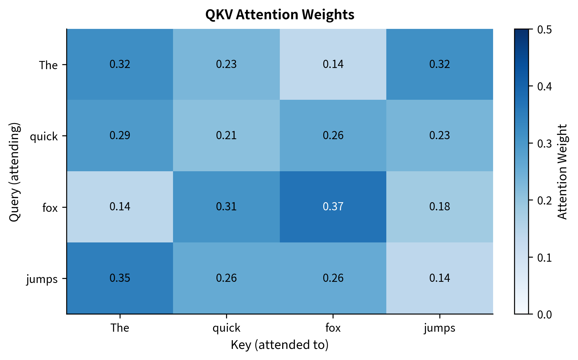
The heatmap shows how each word's query matches against all keys. Each row sums to 1.0 because softmax normalizes the weights. In this random initialization, the patterns aren't meaningful, but after training, we would see linguistically interpretable patterns: articles attending to their nouns, verbs attending to subjects and objects, and so on.
Dimensions and Shapes
Understanding the tensor shapes in self-attention is crucial for implementation and debugging. Let's summarize the key dimensions:
| Tensor | Shape | Description |
|---|---|---|
| Input | tokens, each with -dimensional embedding | |
| Query projection, maps | ||
| Key projection, maps | ||
| Value projection, maps | ||
| Queries | Query vectors for all tokens | |
| Keys | Key vectors for all tokens | |
| Values | Value vectors for all tokens | |
| Scores | All pairwise attention scores | |
| Weights | Softmax-normalized attention | |
| Output | Context-enriched representations |
A few important constraints:
- Query and key dimensions must match () because we compute their dot product
- Value dimension can differ () since values are aggregated, not compared
- Output dimension equals value dimension () because the output is a weighted sum of values
In practice, most implementations set , where is the embedding dimension and is the number of attention heads. This choice ensures that the total computation across all heads remains comparable to a single-head attention with full dimension. We'll explore multi-head attention in a later chapter.
QKV as Learned Transformations
Why do learned projections help? Consider what happens without them. If we use raw embeddings, a word can only attend to other words that happen to have similar embeddings. The word "it" might attend to "this" and "that" (similar pronouns) but struggle to attend to "cat" (semantically relevant but embedding-distant).
With learned projections, the model can discover arbitrary matching patterns. During training:
- learns to transform embeddings into representations that express what each word is looking for
- learns to transform embeddings into representations that advertise what each word offers
- learns what content should actually flow when attention is paid
These projections operate independently, so a word's query doesn't need to resemble its key or value. A pronoun's query might encode "seeking a noun phrase antecedent" while its key might encode "available for coreference" and its value might encode its referent-neutral semantic content.
Let's visualize how the same embeddings project differently into query, key, and value spaces:
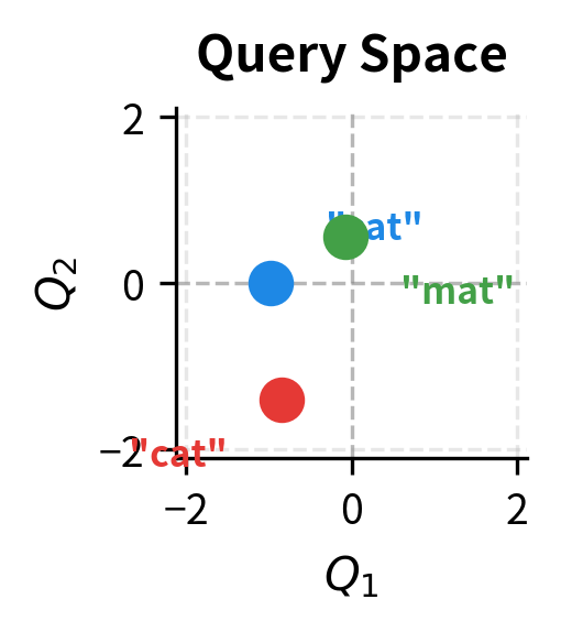
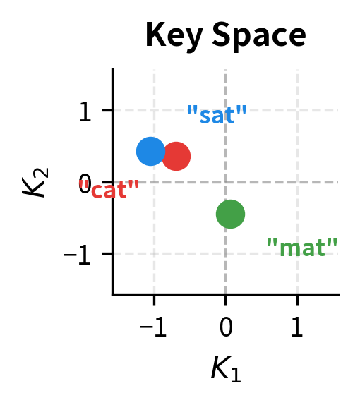
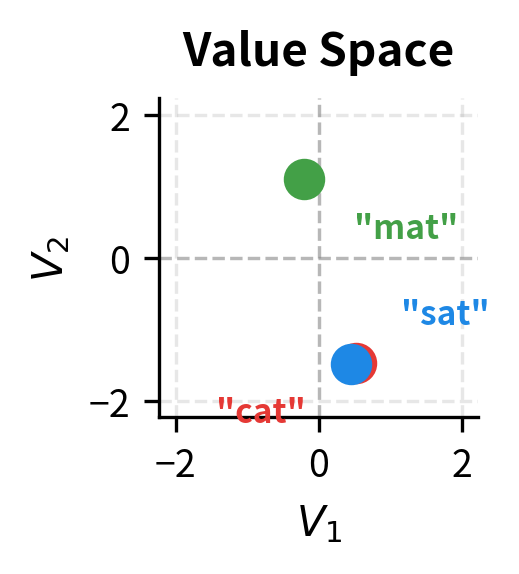
The three projections arrange the same words differently. In query space, the positions reflect what each word is searching for. In key space, positions reflect how words present themselves to queries. In value space, positions determine what gets aggregated. A word might be close to another in query space (they look for similar things) but far in value space (they contribute different content).
Putting It All Together
We've now built up all the components of QKV attention: projections that create specialized representations, dot products that measure compatibility, scaling that ensures stable gradients, and value aggregation that transmits information. Let's combine these into a complete self-attention layer:
The attention weights matrix reveals the core of what self-attention computes: a soft routing table that determines how information flows between positions. Each row sums to exactly 1.0 (confirming proper softmax normalization), and each entry indicates how much one position attends to another.
With random initialization, these patterns are meaningless, just noise from the random projection matrices. But after training on language data, we would see interpretable patterns emerge: determiners attending to nouns, verbs gathering information from subjects and objects, pronouns reaching back to their antecedents.
A Worked Example with Real Words
To make these abstractions concrete, let's trace through QKV attention step by step with a meaningful sentence. We'll use deliberately small embeddings (4 dimensions) and projection matrices (projecting to 3 dimensions) so we can follow every number through the computation.
We've designed these embeddings to be interpretable: each dimension corresponds to a linguistic feature. "The" is a pure determiner (1.0 only in the determiner dimension). "cat" is primarily a noun with high animacy. "sat" is a pure verb. In real systems, embeddings would be dense vectors where meaning is distributed across dimensions, but our hand-crafted features help us trace what the projections do.
Step 1: Computing QKV Projections. The projection matrices transform these 4D embeddings into 3D query, key, and value vectors:
Observe that each word now has three different representations. The same embedding for "cat" becomes different vectors in query, key, and value spaces. This is the core of the QKV framework: specialized representations for specialized roles.
With random projection matrices (as we have here), the vectors don't encode anything linguistically meaningful. But the structure is in place: if we trained these projections on language data, "cat"'s query might learn to seek modifiers and related nouns, its key might learn to signal "available as subject/object," and its value might carry semantic features worth transmitting.
Step 2: Computing Scaled Attention Scores. Now we compute how well each query matches each key:
The raw scores are dot products between query and key vectors. Each entry measures how well one word's query aligns with another word's key. Scaling by compresses the score range, preventing the softmax saturation we discussed earlier.
Notice the variety in scores: some query-key pairs produce positive scores (the vectors point in similar directions), while others produce negative scores (opposing directions). This variety is what allows attention to be selective, with some positions receiving high attention while others receive little.
Step 3: Converting Scores to Attention Weights. Softmax transforms these real-valued scores into a probability distribution:
Each row now sums to exactly 1.0, making these valid probability distributions. The exponential in softmax amplifies differences: a score of 0.5 doesn't just beat 0.3 by a little. It gets substantially more weight after exponentiation. This creates soft but focused attention patterns.
Reading the table: "The" attends to all three words with weights shown in its row. "cat" distributes its attention differently. "sat" has its own pattern. These weights will determine how value vectors are blended to produce each word's output.
Step 4: Aggregating Values into Outputs. Finally, we use the attention weights to compute weighted sums of value vectors:
Each word's output is now a blend of all value vectors, weighted by the attention distribution. The equations show which contributions dominate, displaying only weights above 0.1 to focus on the meaningful contributions.
This is the essence of self-attention: each position receives a custom mixture of information from the entire sequence. The original embedding for "sat" knew nothing about what subject performed the action. After attention, "sat"'s representation incorporates information from "cat" (and "The"), creating a contextualized representation that encodes not just "sat" but "sat with cat as subject in a determined noun phrase."
In trained models, these patterns become linguistically meaningful: verbs attend to their arguments, modifiers attend to what they modify, and pronouns attend to their antecedents, all learned automatically from data without explicit linguistic supervision.
Limitations and Impact
The QKV framework transformed how attention mechanisms are designed. By separating the roles of querying, being queried, and contributing content, it provides flexibility that raw embedding comparisons cannot match. Modern transformers rely entirely on QKV attention, with the projection matrices learning task-specific patterns.
The key limitations stem from the mechanism's simplicity. The projections are linear transformations, meaning the model can only learn linear relationships between embedding dimensions and QKV roles. Deep transformer networks address this by stacking multiple attention layers with nonlinear feed-forward networks between them, allowing the composition of linear attention operations to approximate complex functions.
Another limitation is the lack of explicit structure. QKV attention treats all positions symmetrically, with no built-in notion of syntax, hierarchy, or compositional structure. The model must learn these patterns from data, which requires substantial training examples. This data hunger is both a limitation (large datasets required) and a strength (the model isn't constrained by human-designed rules).
The impact of QKV attention extends beyond NLP. The same mechanism powers vision transformers (ViT), which treat image patches as "tokens." It underlies multimodal models that attend across text, images, and other modalities. The generality of query-key-value matching as a computational primitive has made it foundational across modern AI.
Key Parameters
When implementing QKV self-attention, these parameters control the mechanism's capacity and computational cost:
-
embed_dim(d): The dimension of input token embeddings. This determines the input size to the projection matrices. Common values range from 256 to 4096 in production transformers. -
d_k(query/key dimension): The dimension of query and key vectors after projection. Smaller values reduce computation (since attention scores require operations) but limit the expressiveness of query-key matching. Typically set toembed_dim / num_headsin multi-head attention. -
d_v(value dimension): The dimension of value vectors after projection. This determines the output dimension of the attention layer. Usually equalsd_kfor simplicity, but can differ when the output needs a different size than the matching space. -
Initialization scale: The projection matrices are typically initialized with small random values. Xavier/Glorot initialization scales weights by , where is the input dimension and is the output dimension. This scaling helps maintain stable gradient magnitudes during training by keeping the variance of activations approximately constant across layers.
The ratio of d_k to embed_dim represents a compression factor. Setting d_k < embed_dim forces the model to learn a compressed representation for matching, which can act as a form of regularization. Setting d_k = embed_dim preserves full expressiveness but increases memory and computation.
Summary
Query, Key, Value projections transform self-attention from a fixed similarity computation into a learned matching mechanism. By giving each token separate representations for different roles, the model can learn arbitrary attention patterns that capture linguistic relationships.
Key takeaways from this chapter:
-
Three roles, one mechanism: Queries express what a token seeks, keys advertise what a token offers, and values provide what gets aggregated. This separation enables flexible, learned attention patterns.
-
Projection matrices are learned: , , and are the trainable parameters. During training, they discover which aspects of embeddings matter for matching and aggregation.
-
Query-key matching determines attention: The dot product computes compatibility scores. High scores mean a query matches a key well, leading to high attention weight.
-
Scaling prevents gradient issues: Dividing by keeps score magnitudes stable regardless of dimension, ensuring softmax operates in a regime with healthy gradients.
-
Values carry the content: Attention weights determine how much each position contributes, but value vectors determine what content flows. A token can have a key that attracts attention while its value transmits different information.
-
Dimensions have meaning: Query and key dimensions must match () for dot product compatibility. Value dimension () determines output size. In practice, for simplicity.
In the next chapter, we'll explore multi-head attention, which runs multiple QKV attention operations in parallel. This allows the model to capture different types of relationships simultaneously, dramatically increasing the expressiveness of the attention mechanism.
Quiz
Ready to test your understanding? Take this quick quiz to reinforce what you've learned about the Query, Key, Value mechanism in self-attention.

Comments