Multi-Head Attention: Parallel Attention for Richer Representations

In the previous chapters, we built up the complete picture of scaled dot-product attention: how queries match with keys, how values get aggregated, and how masking controls information flow. A single attention mechanism can capture one type of relationship between tokens. But language is rich with multiple simultaneous relationships. When reading "The cat sat on the mat because it was tired," you simultaneously track syntactic structure (subject-verb agreement), semantic relationships (what "it" refers to), and positional patterns (nearby words). Can we design attention to capture all of these at once?

Multi-head attention answers this question by running multiple attention operations in parallel, each with its own learned projections. Instead of one attention mechanism looking for one type of pattern, we have several "heads," each specializing in different aspects of the input. This architectural choice is central to transformer performance and appears in every major language model from BERT to GPT-4.

Single-head attention computes one set of attention weights per position. Each token decides how to weight all other tokens, producing a single blended representation. This works well for capturing one dominant relationship, but it forces a choice: should "sat" attend mostly to its subject "cat," its location "mat," or its tense indicators?

Consider a more complex example: "The lawyer who the witness saw left." To parse this sentence correctly, a model must simultaneously track multiple dependencies. "Who" relates back to "lawyer" (as an antecedent). "Saw" connects to "witness" (as its subject) and to "who" (as its object). "Left" connects back to "lawyer" (not "witness") as its subject. A single attention head must somehow encode all these relationships in one set of weights.

The solution is straightforward: instead of computing attention once, compute it multiple times with different projections. Each "head" learns to focus on different aspects of the input. One head might specialize in syntactic relationships, another in coreference, and another in local context. By combining their outputs, the model builds a richer representation than any single head could achieve.

Multi-head attention divides the model's capacity across $h$ parallel attention heads. Each head operates on a reduced dimension, so the total computation remains comparable to single-head attention with the full dimension.

The process unfolds in four steps:

1. Project the input into $h$ separate query, key, and value representations
2. Compute scaled dot-product attention independently for each head
3. Concatenate all head outputs into a single tensor
4. Project the concatenated output back to the model dimension

Let's trace through each step with concrete mathematics and then implement it in code.

Given an input sequence $\mathbf{X} \in \mathbb{R}^{n \times d_{\text{model}}}$ with $n$ tokens and model dimension $d_{\text{model}}$, we project it into queries, keys, and values for each head. If we have $h$ heads, we typically set the head dimension to $d_k = d_{\text{model}} / h$. This division ensures that the total computation across all heads remains comparable to a single attention operation over the full dimension.

For head $i$, we compute the query, key, and value matrices through learned linear projections:

where:

• $\mathbf{X} \in \mathbb{R}^{n \times d_{\text{model}}}$: the input sequence with $n$ tokens, each represented as a $d_{\text{model}}$-dimensional vector
• $\mathbf{W}^Q_i \in \mathbb{R}^{d_{\text{model}} \times d_k}$: the learned query projection matrix for head $i$, transforming each token into a $d_k$-dimensional query vector
• $\mathbf{W}^K_i \in \mathbb{R}^{d_{\text{model}} \times d_k}$: the learned key projection matrix for head $i$, transforming each token into a $d_k$-dimensional key vector
• $\mathbf{W}^V_i \in \mathbb{R}^{d_{\text{model}} \times d_v}$: the learned value projection matrix for head $i$ (often $d_v = d_k$)
• $\mathbf{Q}_i, \mathbf{K}_i \in \mathbb{R}^{n \times d_k}$: the resulting query and key matrices for head $i$
• $\mathbf{V}_i \in \mathbb{R}^{n \times d_v}$: the resulting value matrix for head $i$
• $d_k$: the per-head dimension, typically $d_{\text{model}} / h$

Each head gets its own projection matrices, allowing it to learn different transformations of the input. Head 1 might project tokens to emphasize syntactic features, while head 2 emphasizes semantic similarity. The key insight is that different projection matrices create different "views" of the same input, each potentially highlighting different aspects of the token relationships.

Each head computes standard scaled dot-product attention using its own projections. The attention mechanism compares queries against keys to determine relevance weights, then uses those weights to aggregate values:

where:

• $\text{head}_i \in \mathbb{R}^{n \times d_v}$: the output of attention head $i$, containing contextual representations for all $n$ tokens
• $\mathbf{Q}_i \mathbf{K}_i^T \in \mathbb{R}^{n \times n}$: the matrix of raw attention scores, where entry $(j, k)$ measures how much query at position $j$ matches key at position $k$
• $\sqrt{d_k}$: the scaling factor that prevents dot products from growing too large as $d_k$ increases (covered in the previous chapter on scaled dot-product attention)
• $\text{softmax}(\cdot)$: applied row-wise to convert scores into attention weights that sum to 1 for each query position
• $\mathbf{V}_i$: the value matrix whose rows are aggregated according to the attention weights

This produces $h$ separate outputs, each of shape $\mathbb{R}^{n \times d_v}$. The heads operate completely independently at this stage; there is no information sharing between them. This independence is what allows different heads to specialize in detecting different types of relationships.

After computing all heads, we concatenate their outputs along the feature dimension. Each head produces an $n \times d_v$ matrix, and stacking these side-by-side creates a larger matrix:

where:

• $\text{head}_1, \ldots, \text{head}_h$: the $h$ individual head outputs, each of shape $\mathbb{R}^{n \times d_v}$
• $h \cdot d_v$: the concatenated feature dimension, combining all heads' outputs

If $d_v = d_k = d_{\text{model}} / h$, then $h \cdot d_v = d_{\text{model}}$, and the concatenated output has the same dimension as the original input. This dimensional consistency is intentional: it allows multi-head attention to be used as a drop-in replacement for single-head attention. The concatenation preserves each head's contribution separately, letting the subsequent projection learn how to combine them.

Finally, we apply a learned linear projection to the concatenated output. This projection maps the combined head outputs back to the model dimension:

where:

• $\text{Concat}(\text{head}_1, \ldots, \text{head}_h) \in \mathbb{R}^{n \times (h \cdot d_v)}$: the concatenated outputs from all $h$ attention heads
• $\mathbf{W}^O \in \mathbb{R}^{(h \cdot d_v) \times d_{\text{model}}}$: the learned output projection matrix
• $\text{MultiHead}(\mathbf{X}) \in \mathbb{R}^{n \times d_{\text{model}}}$: the final output, matching the input dimension

This projection serves two purposes. First, it combines information from all heads, allowing the model to learn how to mix their contributions. A head specializing in syntax might contribute more heavily for certain tokens, while a semantic head dominates for others. Second, it ensures the output dimension matches the input dimension, enabling residual connections in the transformer architecture.

Now that we've walked through each step conceptually, let's see how they combine into a complete formulation. Understanding this picture helps clarify how multi-head attention works: by running multiple specialized attention operations in parallel and learning to combine their insights.

The outer structure of multi-head attention takes the outputs from all heads and merges them:

This formula reads from inside out: first compute each head, then concatenate their outputs, then apply the output projection. But what exactly is each head doing? Each head applies its own learned projections before computing attention:

where:

• $\mathbf{Q}, \mathbf{K}, \mathbf{V}$: the query, key, and value inputs (in self-attention, all three equal the input $\mathbf{X}$)
• $\mathbf{W}^Q_i, \mathbf{W}^K_i, \mathbf{W}^V_i$: the per-head projection matrices for head $i$, each transforming the full $d_{\text{model}}$-dimensional input into a smaller $d_k$-dimensional subspace
• $\text{Attention}(\cdot)$: the scaled dot-product attention function from the previous chapter
• $\mathbf{W}^O$: the output projection that learns how to combine all heads' contributions

The design is flexible. In self-attention, $\mathbf{Q} = \mathbf{K} = \mathbf{V} = \mathbf{X}$, so the same input sequence projects to all three roles. But the same multi-head attention mechanism also supports cross-attention in encoder-decoder models, where queries come from the decoder and keys/values come from the encoder. The mathematical structure remains identical; only the inputs differ.

Why should projecting to lower-dimensional subspaces and computing attention there be useful? Think of it this way: the full $d_{\text{model}}$-dimensional embedding space contains many different types of information about each token. Its syntactic role, semantic meaning, position in the sentence, relationship to neighboring words. A single attention operation in the full space must somehow balance all of these considerations when deciding what to attend to.

By projecting to a lower-dimensional subspace, each head can focus on a particular "slice" of the information. One head's projection matrices might learn to emphasize dimensions that capture syntactic structure, causing that head to attend based on grammatical relationships. Another head's projections might emphasize semantic dimensions, causing it to attend based on meaning similarity. The output projection then learns to weigh and combine these different perspectives.

This is analogous to how ensemble methods work in machine learning: multiple weak learners, each capturing part of the pattern, combine to form a stronger predictor than any single model could achieve.

A natural question arises: if we're running $h$ separate attention operations, doesn't that multiply our parameter count by $h$? Actually, no. The dimension splitting ensures that multi-head attention uses approximately the same number of parameters as single-head attention with the full dimension.

Let's trace through the calculation:

1. Per head: Each head has three projection matrices ($\mathbf{W}^Q_i$, $\mathbf{W}^K_i$, $\mathbf{W}^V_i$), each of size $d_{\text{model}} \times d_k$. That's $3 \times d_{\text{model}} \times d_k$ parameters per head.

2. All heads: With $h$ heads, we multiply by $h$: total QKV parameters are $h \times 3 \times d_{\text{model}} \times d_k$. Here's the key insight: since $d_k = d_{\text{model}} / h$, we have $h \times d_k = d_{\text{model}}$. This simplifies our expression to $3 \times d_{\text{model}}^2$.

3. Output projection: The matrix $\mathbf{W}^O$ has size $(h \cdot d_v) \times d_{\text{model}}$. With $d_v = d_k = d_{\text{model}} / h$, the input dimension is $h \cdot (d_{\text{model}} / h) = d_{\text{model}}$, giving us $d_{\text{model}} \times d_{\text{model}} = d_{\text{model}}^2$ parameters.

4. Grand total: $3 \times d_{\text{model}}^2 + d_{\text{model}}^2 = 4 \times d_{\text{model}}^2$ parameters.

This is exactly what we'd have with single-head attention using the full dimension, plus one additional output projection. The key benefit of multi-head attention is that we get $h$ different attention patterns, each potentially specializing in different relationships, for essentially the same parameter budget as a single larger head.

With the mathematics clear, let's translate these ideas into working code. We'll build multi-head attention from scratch using NumPy, making every operation explicit so you can see exactly how the formulas map to implementation. This hands-on approach will solidify your understanding and prepare you to work with production implementations in PyTorch or TensorFlow.

Our implementation needs two building blocks: first, the scaled dot-product attention we covered in the previous chapter; second, the multi-head wrapper that orchestrates multiple attention operations in parallel.

We start with a function that computes attention for tensors that already include a head dimension. This allows us to process all heads simultaneously through batched matrix multiplication:

Notice the tensor shape: (batch, heads, seq_len, d_k). By placing the head dimension second, we can compute attention scores for all heads at once. The matrix multiplication Q @ K.transpose(...) produces a (batch, heads, seq_len, seq_len) tensor containing $h$ separate attention matrices, one per head. This is the key to efficient parallel computation.

Now we build the main module. The MultiHeadAttention class encapsulates all the projection matrices and orchestrates the four-step process we described earlier.

A key implementation detail: instead of storing separate $\mathbf{W}^Q_i$, $\mathbf{W}^K_i$, $\mathbf{W}^V_i$ matrices for each head, we use a single combined projection matrix W_qkv of shape (d_model, 3 * d_model). This computes all queries, keys, and values for all heads in one matrix multiplication. The result is then split and reshaped to separate the heads. This approach is more efficient on GPUs because it maximizes parallelism and minimizes memory transfers.

The split_heads and combine_heads methods handle the tensor reshaping that makes parallel head computation possible. split_heads takes a tensor of shape (batch, seq_len, d_model) and reorganizes it to (batch, num_heads, seq_len, d_k), separating the head dimension. combine_heads reverses this transformation after attention is computed.

Let's verify our implementation produces the expected output shapes and that the attention weights are properly normalized:

The output tensor has shape (1, 6, 64), matching the input exactly. This dimensional consistency is essential for residual connections in transformer architectures. The attention weights have shape (1, 4, 6, 6), representing a separate $6 \times 6$ attention matrix for each of the 4 heads.

Each row sums to exactly 1.0, confirming that softmax normalization is working correctly. This is expected: for each query position, the attention weights across all key positions must form a valid probability distribution.

Let's visualize how multi-head attention changes the token representations. We'll use PCA to project the 64-dimensional embeddings down to 2D, allowing us to see how the representations shift after passing through the attention layer.

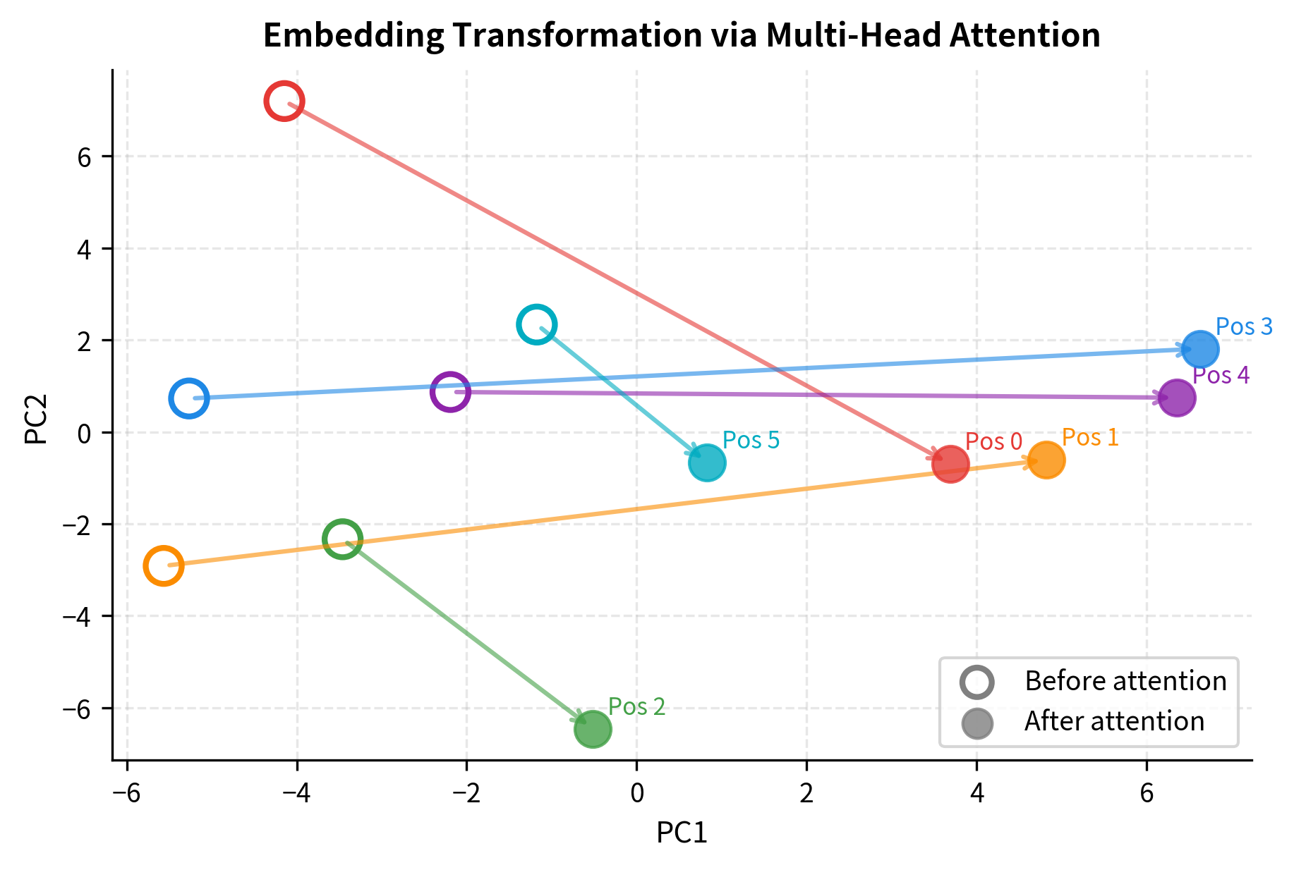
The visualization shows how multi-head attention repositions each token's representation in embedding space. The arrows indicate the direction and magnitude of change. Tokens that attended strongly to semantically related positions move toward each other, while tokens that focused on different aspects of the input shift in different directions. This is the contextual enrichment in action: each position now carries information gathered from across the sequence.

The true power of multi-head attention becomes apparent when we visualize what different heads are doing. Even with random initialization (before any training), the different projection matrices cause each head to compute different attention patterns. After training on language data, these patterns become meaningful: heads specialize to detect specific types of relationships.

Let's visualize the attention patterns for each head on a simple sentence. We'll create random embeddings and see how the four heads distribute their attention differently:

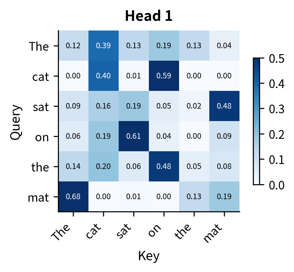
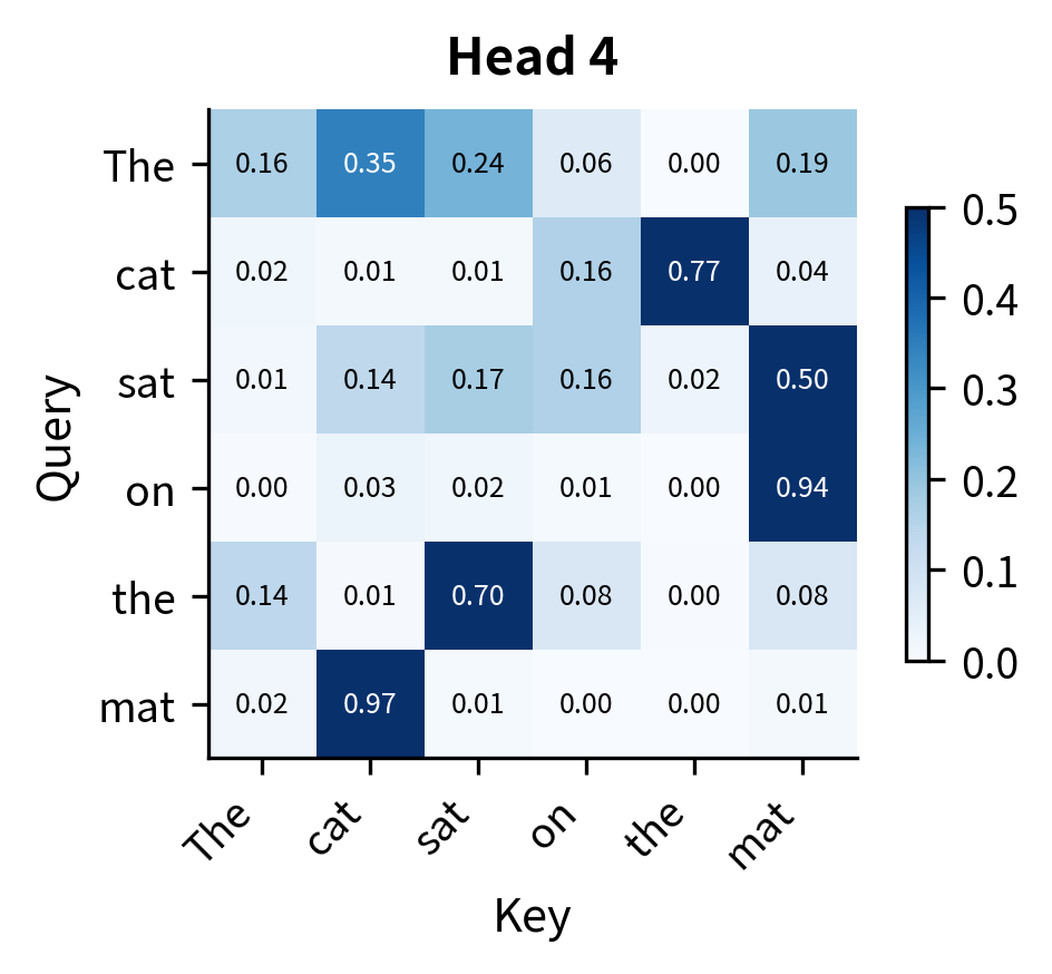
The heatmaps reveal that even with random initialization, each head produces a distinct attention pattern. Some heads distribute attention more uniformly, while others concentrate it on specific positions. In a trained model, these differences become meaningful and interpretable: one head might consistently attend to the previous word (useful for language modeling), another to syntactically related words (useful for parsing), and another to semantically similar words (useful for coreference resolution).

The key observation is that the same input, "The cat sat on the mat," produces four different perspectives on token relationships. This diversity is precisely what we wanted when we motivated multi-head attention: the ability to capture multiple types of dependencies simultaneously.

We can quantify how "focused" or "distributed" each head's attention is using entropy. A head with low entropy concentrates attention on a few positions, while a head with high entropy distributes attention more uniformly. This provides a numerical measure of the diversity we observed visually.

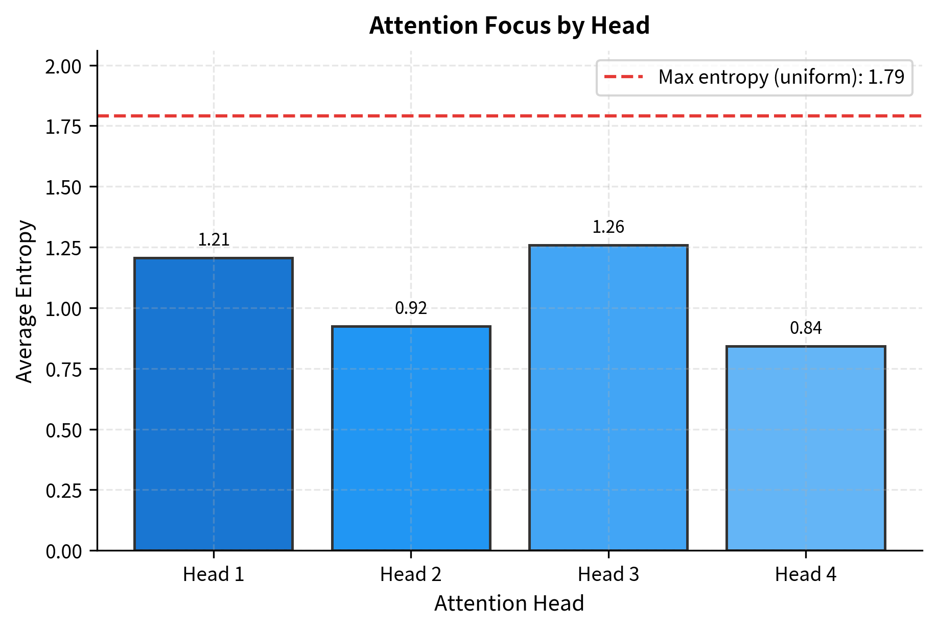
Heads with lower entropy relative to the maximum are more "focused," concentrating their attention on specific positions. Heads closer to the maximum entropy distribute attention more uniformly. This variation in focus is another dimension of head diversity: some heads act as sharp selectors, while others aggregate information more broadly.

Research on trained transformers reveals that attention heads develop distinct specializations. Some commonly observed patterns include:

• Positional heads: Attend to fixed relative positions (e.g., always attend to the previous token, or always attend to the first token)
• Syntactic heads: Track grammatical relationships like subject-verb or modifier-noun connections
• Coreference heads: Link pronouns to their antecedents across the sequence
• Rare word heads: Focus on infrequent tokens that carry high information content
• Separator heads: Attend to punctuation and sentence boundaries

This specialization emerges purely from training on language modeling objectives. No explicit supervision tells heads what to focus on; they discover useful patterns through gradient descent.

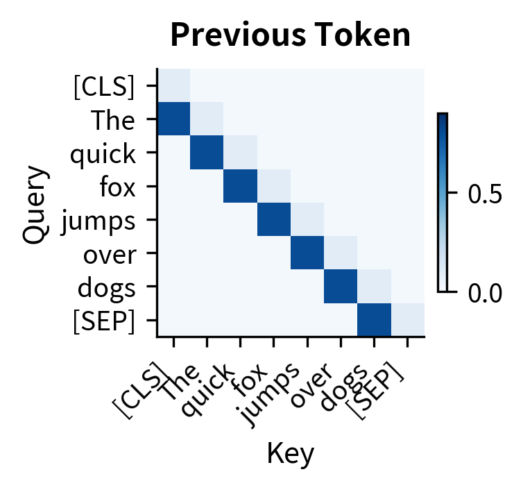
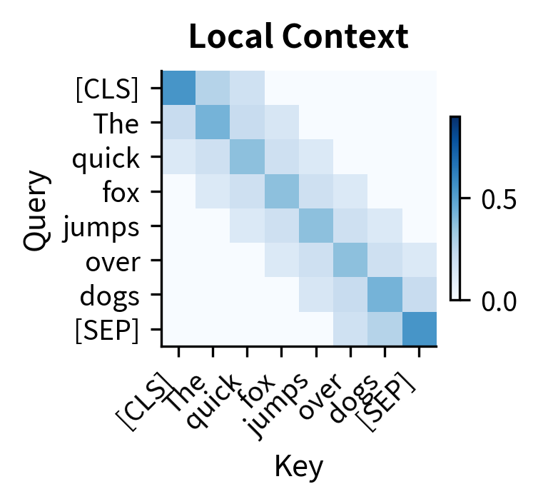
The three patterns illustrate different specializations:

• Previous token head: The diagonal pattern shows each token attending primarily to its predecessor. This captures local sequential dependencies, useful for language modeling where the previous word strongly predicts the next.

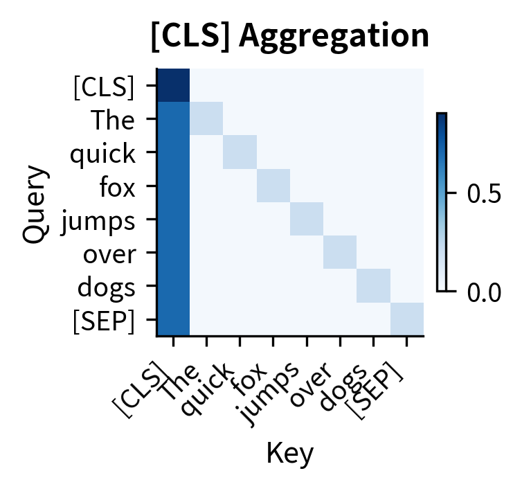
• [CLS] aggregation head: The first column lights up, showing all tokens attending to the special classification token. This pattern aggregates information from the entire sequence into one position, commonly used for classification tasks.

• Local context head: The banded pattern shows attention concentrated within a local window. This captures phrase-level relationships without being distracted by distant tokens.

How much does multi-head attention actually help? Let's compare the representational capacity of single-head versus multi-head attention on a simple task: capturing diverse pairwise relationships.

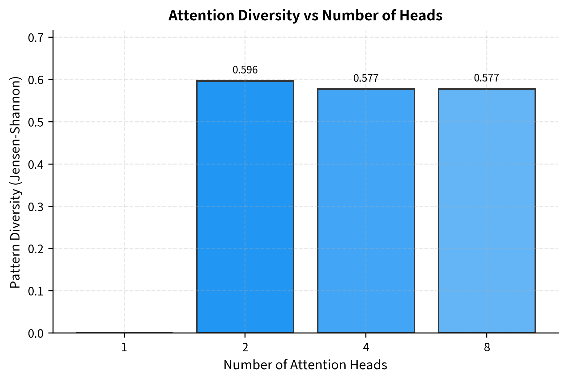
The diversity metric reveals a clear pattern: more heads lead to more varied attention patterns. With a single head, the diversity score is 0 by definition since there's nothing to compare. With 2 heads, the model can already capture distinct patterns. As we increase to 4 and 8 heads, diversity continues to grow, though the incremental gains diminish. This suggests that beyond a certain point, additional heads may begin to learn redundant patterns.

When implementing multi-head attention in production systems, several practical considerations come into play.

The original transformer paper used 8 heads with a 512-dimensional model, giving each head 64 dimensions. Modern large models often use more heads, but the per-head dimension typically stays between 64 and 128.

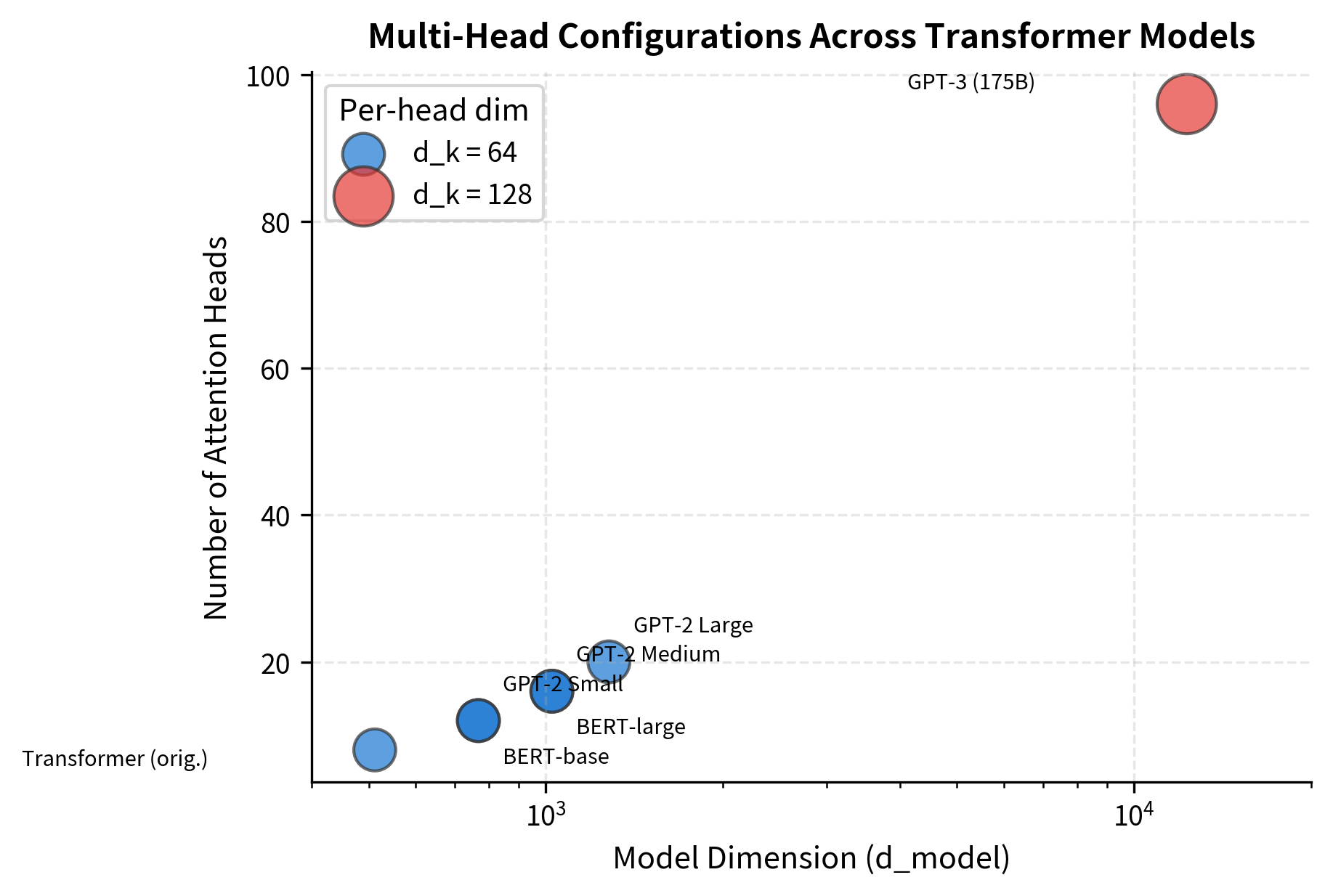
The visualization reveals a consistent design pattern: as model dimension increases, the number of heads scales proportionally to maintain per-head dimensions between 64 and 128. This suggests an empirically validated "sweet spot" for head expressiveness. Too few dimensions per head limit each head's ability to capture complex patterns; too many heads with too few dimensions fragment the representation unhelpfully.

Although multi-head attention computes $h$ separate attention operations, modern implementations parallelize this efficiently. The key insight is that we can stack all heads into a single tensor and use batched matrix multiplication.

This batched approach processes all heads with the same matrix operations, leveraging GPU parallelism. The computational cost is essentially equivalent to single-head attention with some reshaping overhead.

Research has shown that not all attention heads are equally important. Some heads can be removed after training with minimal impact on performance. This head pruning technique reduces computation and memory for inference.

Studies on BERT found that many heads could be pruned without significant accuracy loss, suggesting some redundancy in the learned representations. This has practical implications for deploying models in resource-constrained environments.

Multi-head attention is one of the key innovations that made transformers successful. By allowing the model to jointly attend to information from different representation subspaces at different positions, it provides a flexible mechanism for capturing complex relationships in language. Each head learns its own projection matrices, creating specialized views of the input that combine to form rich contextual representations.

The primary limitation is computational. Multi-head attention still has $O(n^2)$ complexity in sequence length $n$, and the overhead of multiple heads adds constant factors to both computation and memory. For a sequence of 4,096 tokens with 32 heads, the model must compute and store 32 separate attention matrices, each of size $4096 \times 4096$. This quadratic scaling remains a bottleneck for very long documents, motivating research into efficient attention variants like sparse attention (which attends to a subset of positions), linear attention (which reformulates the computation to avoid explicit attention matrices), and methods like FlashAttention (which optimizes memory access patterns).

Another consideration is interpretability. While we can visualize attention patterns, understanding what each head has learned remains challenging. Research has shown that some heads appear redundant, attending to similar patterns, while others develop specializations that don't correspond to human-interpretable categories. This makes it difficult to debug unexpected model behavior or explain predictions. The observation that many heads can be pruned without significant accuracy loss suggests that multi-head attention may include built-in redundancy, which could be beneficial for robustness but represents inefficiency during inference.

Despite these limitations, multi-head attention works well across virtually all NLP tasks. The ability to capture multiple types of relationships simultaneously, without explicit supervision about what those relationships should be, is a key reason why transformers generalize so well. From named entity recognition to machine translation to question answering, multi-head attention provides the representational flexibility needed to handle diverse linguistic phenomena.

When configuring multi-head attention, the following parameters have the most significant impact on model behavior:

• num_heads (h): The number of parallel attention heads. Common values range from 8 to 96 depending on model size. More heads enable greater specialization but require the model dimension to be evenly divisible. Start with 8 heads for smaller models and scale proportionally with model dimension.

• d_model: The model dimension, which determines the total representation capacity. Must be divisible by num_heads. Standard values include 512 (original transformer), 768 (BERT-base), 1024 (BERT-large), and 12288 (GPT-3).

• d_k (head dimension): The dimension per head, computed as d_model // num_heads. Values between 64 and 128 work well in practice. Smaller values allow more heads but limit each head's expressiveness.

• d_v (value dimension): Often set equal to d_k. Can be set independently if you want asymmetric query-key versus value dimensions, though this is uncommon.

• Initialization scale: Projection matrices are typically initialized with variance $\frac{2}{d_{\text{model}}}$ or similar schemes. Poor initialization can cause attention weights to become too uniform or too peaked early in training.

Multi-head attention extends single-head attention by running multiple attention operations in parallel, each with its own learned projections. This architectural choice significantly impacts model capacity and performance.

Key takeaways from this chapter:

• Parallel heads: Multi-head attention computes $h$ independent attention operations, each learning different relationship patterns between tokens. Each head can specialize in detecting specific linguistic phenomena.
• Dimension splitting: The model dimension $d_{\text{model}}$ is divided among heads, with each head operating on dimension $d_k = d_{\text{model}} / h$. This keeps total computation comparable to single-head attention while enabling multiple perspectives.
• Four-step process: (1) Project input to Q, K, V for each head using learned matrices $\mathbf{W}^Q_i$, $\mathbf{W}^K_i$, $\mathbf{W}^V_i$; (2) compute scaled dot-product attention independently per head; (3) concatenate head outputs; (4) apply final output projection $\mathbf{W}^O$.
• Head specialization: Different heads learn to focus on different aspects: positional patterns, syntactic relationships, semantic similarity, or coreference links. This emerges from training without explicit supervision.
• Parameter efficiency: The total parameter count is $4 \times d_{\text{model}}^2$, similar to single-head attention with an output projection. The gain is in representational diversity, not parameter count.
• Practical implementations: Efficient implementations batch all heads into single tensor operations, leveraging GPU parallelism through combined QKV projections.

In the next chapter, we'll examine the computational complexity of attention in detail. Understanding the $O(n^2)$ scaling (where $n$ is sequence length) and its implications is essential for working with long sequences and motivates the efficient attention variants used in modern long-context models.

Ready to test your understanding? Take this quick quiz to reinforce what you've learned about multi-head attention.