

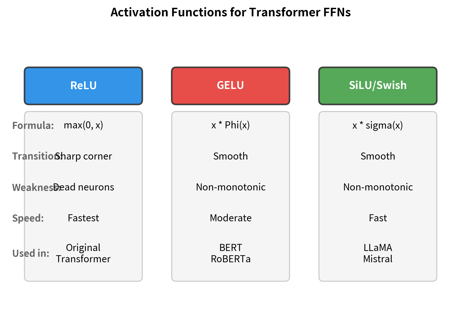
Compare activation functions in transformer feed-forward networks: ReLU's simplicity and dead neuron problem, GELU's smooth probabilistic gating for BERT, and SiLU/Swish for modern LLMs like LLaMA.

This article is part of the free-to-read Language AI Handbook
Choose your expertise level to adjust how many terms are explained. Beginners see more tooltips, experts see fewer to maintain reading flow. Hover over underlined terms for instant definitions.
FFN Activation Functions
The feed-forward network's power comes from its nonlinear activation function. Without nonlinearity, stacking multiple linear layers would collapse into a single linear transformation, no matter how deep the network. The activation function is what enables FFNs to approximate arbitrarily complex functions of language.
The original transformer used ReLU, the workhorse of deep learning since 2012. But as researchers scaled transformers to billions of parameters and trained them on trillions of tokens, subtle differences between activation functions became significant. GELU emerged as the standard for encoder models like BERT. SiLU (also called Swish) now dominates decoder models like LLaMA and GPT-NeoX. Understanding why these activations differ, and when each excels, is essential for building modern language models.
This chapter traces the evolution from ReLU to GELU to SiLU/Swish, examining the mathematical properties that make each function suitable for different contexts. You'll implement each activation, visualize their differences, and understand the practical trade-offs that guide model design choices.
ReLU: The Original Choice
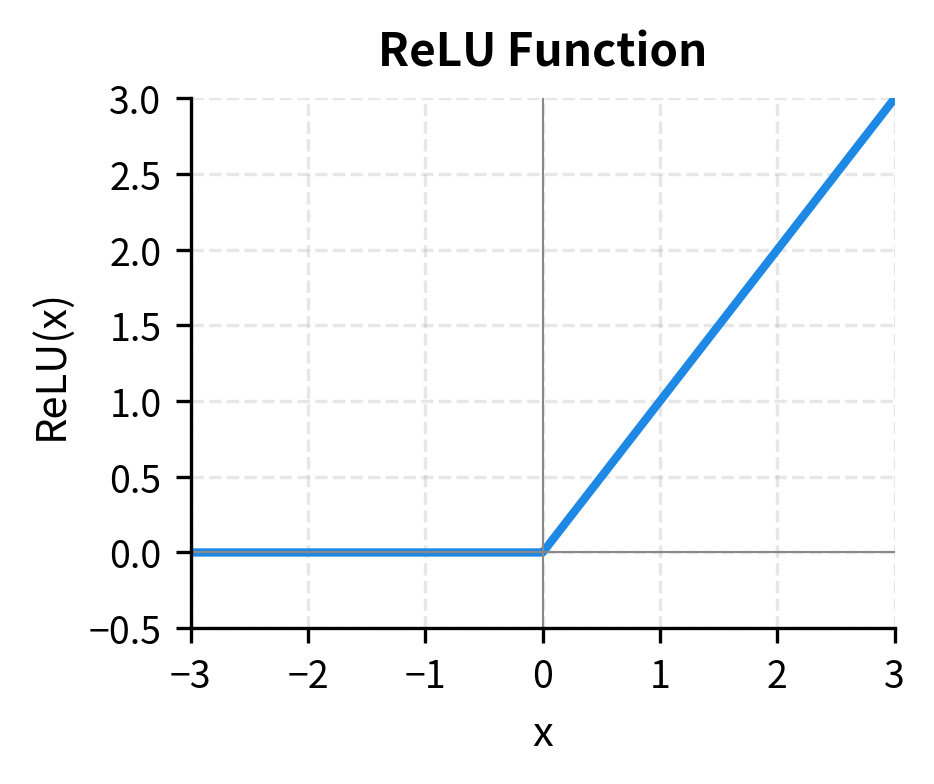
The Rectified Linear Unit (ReLU) is the simplest nonlinear activation function in modern deep learning. It applies a trivial rule: keep positive values unchanged, set negative values to zero. Mathematically:
where:
- : the input value (a single element of the pre-activation vector)
- : returns if , otherwise returns
This simplicity is deceptive. ReLU revolutionized deep learning when introduced in AlexNet (2012), enabling training of much deeper networks than the sigmoid and tanh activations that preceded it. The original transformer adopted ReLU for its feed-forward layers, inheriting this proven workhorse.
A piecewise linear activation function that outputs the input directly if positive, otherwise outputs zero. Its simplicity enables fast computation and its non-saturating positive region prevents vanishing gradients during backpropagation.
Let's implement ReLU and examine its behavior:
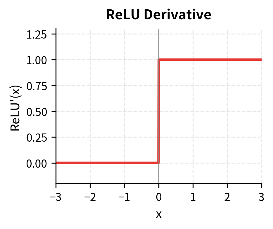
ReLU's advantages are clear. Its computation is trivial: a single comparison operation. The derivative is equally simple:
where:
- The derivative is 1 for positive inputs, meaning gradients flow through unchanged
- The derivative is 0 for negative inputs, meaning gradients are blocked entirely
- The derivative is technically undefined at exactly , but implementations typically use 0 or 1
This step function gradient never vanishes for positive inputs like sigmoid's gradient does for large values. And ReLU creates sparse activations, as roughly half of all hidden units output zero for typical input distributions, which can improve efficiency and interpretability.
The Dead ReLU Problem
But ReLU has a critical weakness. When a neuron's pre-activation is consistently negative, its gradient is always zero. The neuron stops learning entirely. This "dying ReLU" problem becomes more severe as networks deepen or learning rates increase.
Consider what happens during training. If a weight update pushes a neuron's bias too negative, that neuron's output becomes zero for all inputs. With zero output, the gradient flowing through that neuron is zero. With zero gradient, the weights never update. The neuron is dead.
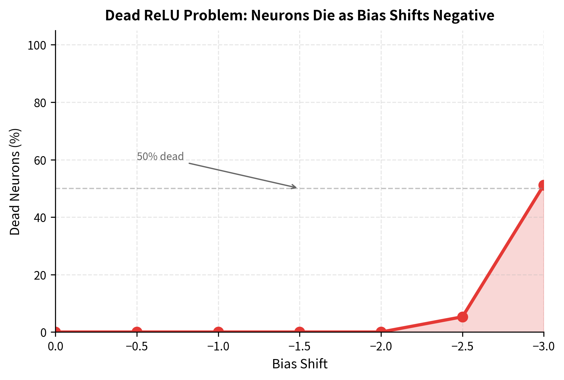
The plot shows how quickly neurons die as bias values shift negative. In real training, this can happen in patches of the network, reducing effective capacity without obvious symptoms. The model trains, but parts of it have effectively disconnected from the computation.
GELU: The Smooth Alternative
Hendrycks and Gimpel introduced the Gaussian Error Linear Unit (GELU) in 2016, though it didn't gain widespread adoption until BERT popularized it in 2018. GELU addresses ReLU's sharp corner by introducing smooth, probabilistic gating.
The intuition behind GELU is elegant: instead of deterministically zeroing negative values, gate each input by its probability of being positive under a standard normal distribution. Inputs that are clearly positive (large positive values) pass through nearly unchanged. Inputs that are clearly negative (large negative values) are nearly zeroed. Inputs near zero, where classification is uncertain, are partially attenuated.
The mathematical formulation follows this intuition:
where:
- : the input value to the activation function
- : the cumulative distribution function (CDF) of the standard normal distribution, representing the probability that a standard normal random variable is less than or equal to
The CDF itself is computed using the error function:
where:
- : the probability that a standard normal random variable takes a value less than or equal to
- : the Gauss error function, a special function that arises in probability and statistics
- : a scaling factor that converts from the standard normal to the error function's parameterization
The CDF ranges from 0 to 1. For large positive , , so . For large negative , , so . The transition is smooth, governed by the bell curve of the normal distribution.
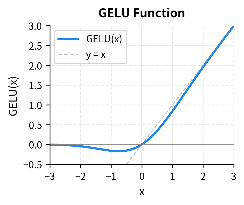
An activation function that gates inputs by their Gaussian CDF values, creating a smooth, non-monotonic function that approximates stochastic regularization. GELU is the standard activation for encoder-style transformers like BERT and RoBERTa.
GELU has a distinctive shape: it's nearly linear for positive values, smoothly transitions through zero, and has a slight dip into negative territory before approaching zero asymptotically. This dip is unique. For small negative inputs (around ), GELU actually outputs slightly negative values. This non-monotonic behavior distinguishes it from ReLU variants.
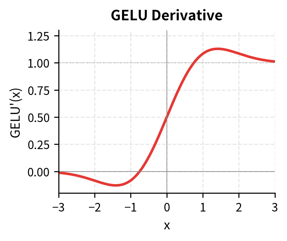
The derivative of GELU, which determines gradient flow during backpropagation, is:
where:
- : the standard normal CDF (as defined above)
- : the standard normal probability density function (PDF)
- The first term contributes the "identity-like" gradient for positive inputs
- The second term creates a smooth transition region and ensures the derivative is continuous everywhere
GELU Approximations
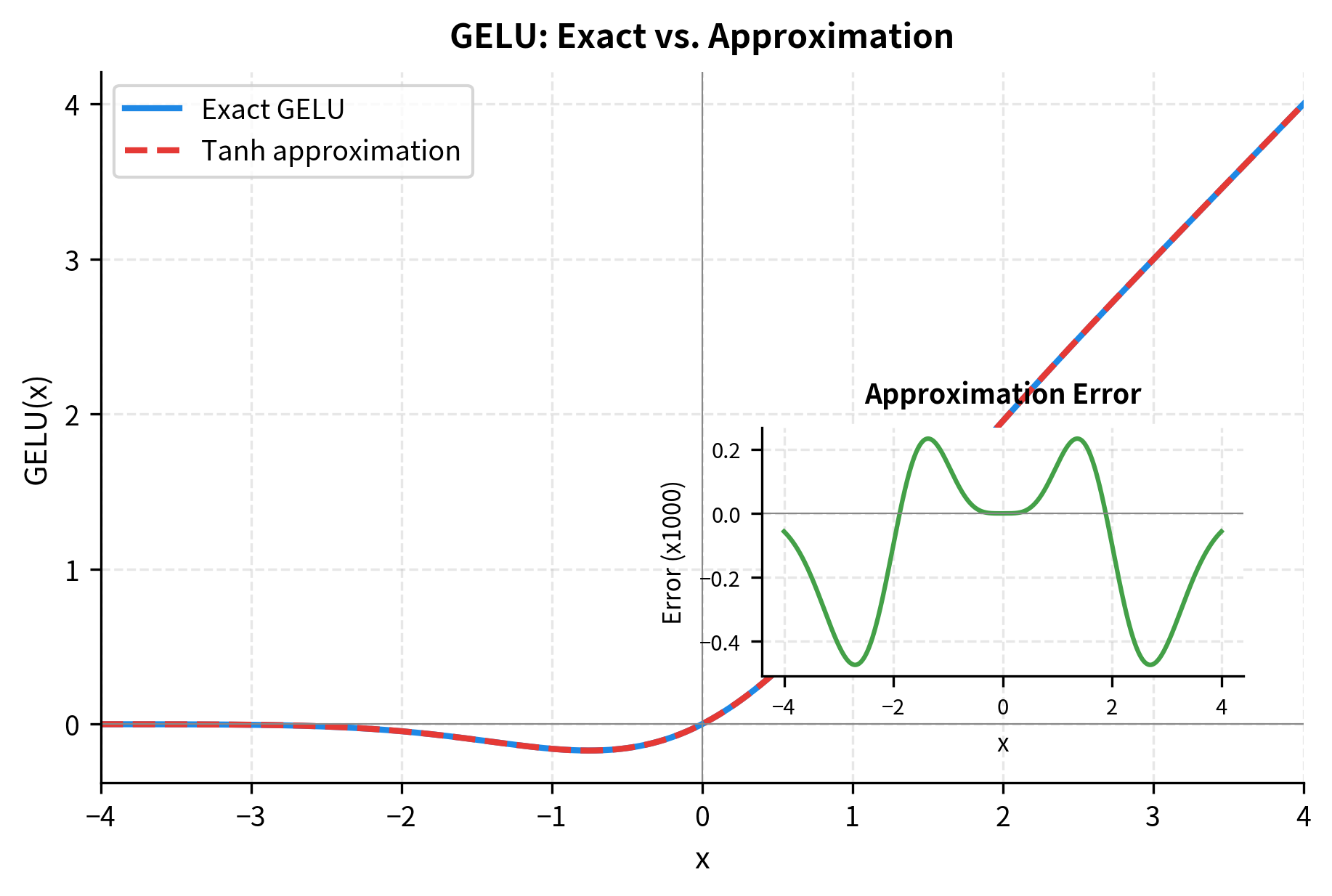
Computing the exact error function is expensive. In practice, transformers use fast approximations. The most common is the tanh approximation:
where:
- : the input value
- : the hyperbolic tangent function, which outputs values in the range
- : a scaling constant derived from properties of the normal distribution
- : an empirically-fitted coefficient that improves the approximation accuracy
- : a polynomial that approximates the argument to the error function
This formula looks complex, but it avoids the expensive erf computation while matching GELU closely. The constants were determined by fitting to the exact GELU curve, minimizing the maximum error across typical input ranges.
Let's compare the exact and approximate versions:
The approximation error is negligible for practical purposes. Most deep learning frameworks offer both versions, with the tanh approximation being faster on hardware that lacks specialized erf instructions.
SiLU/Swish: The Modern Standard
While GELU became the activation of choice for encoder models like BERT, a different function emerged for large decoder models: SiLU, also known as Swish. Google researchers introduced Swish in 2017 through neural architecture search, discovering that this simple formula consistently outperformed ReLU across tasks.
where:
- : the input value
- : the logistic sigmoid function (defined below)
- : the exponential function with negative argument, which rapidly approaches 0 for large positive and infinity for large negative
The sigmoid function that gates the input is:
where:
- : outputs a value in the range , interpretable as a "gate" or probability
- For large positive : , so (input passes through)
- For large negative : , so (input is suppressed)
- At : , so
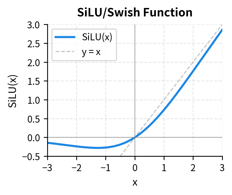
The name "SiLU" stands for Sigmoid Linear Unit, emphasizing its structure: the input multiplied by its sigmoid. "Swish" was Google's original branding. The two names refer to the same function, though the literature isn't always consistent.
An activation function defined as , where is the sigmoid function. SiLU is smooth, non-monotonic, and unbounded above. It has become the standard activation for decoder-style transformers like LLaMA, Mistral, and GPT-NeoX.
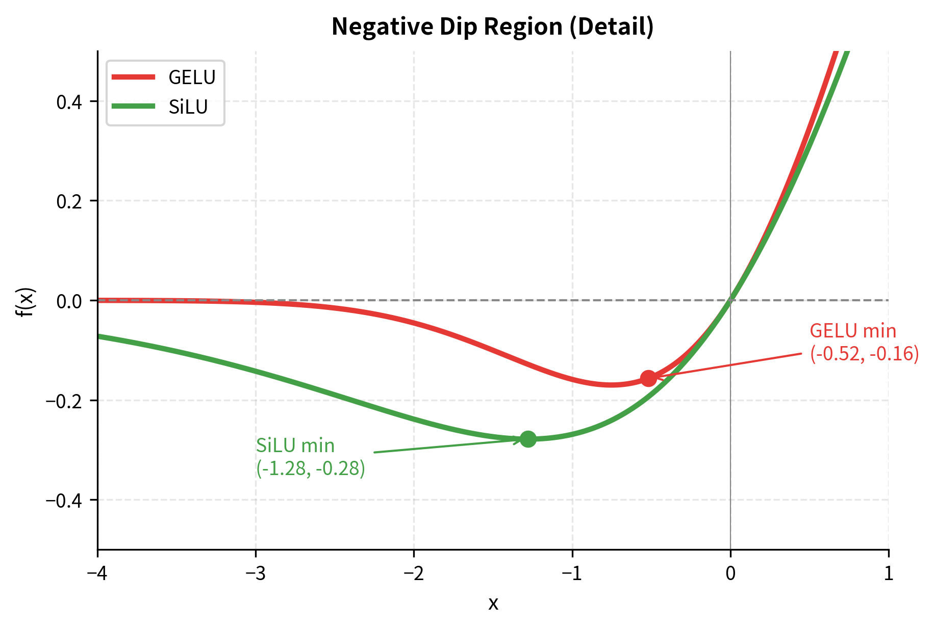
SiLU shares GELU's smooth, non-monotonic character. Both have a slight negative dip, both transition smoothly through zero, and both asymptotically approach the identity for large positive values. But the functions differ subtly: SiLU's dip is slightly deeper (minimum around -0.28 compared to GELU's -0.17), and its transition is slightly sharper.
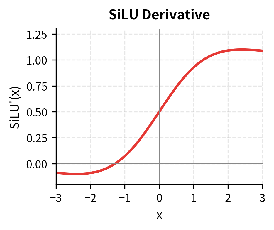
The derivative of SiLU, derived using the product rule, is:
where:
- : the sigmoid function
- : the derivative of the sigmoid, which has a bell-shaped curve centered at
- The first term approaches 1 for large positive , giving gradient 1
- The second term adds a positive contribution near , allowing SiLU's derivative to exceed 1
Why Decoder Models Prefer SiLU
The preference for SiLU in decoder models like LLaMA, Mistral, and Falcon isn't fully understood theoretically, but several factors contribute:
-
Simpler computation: SiLU requires only sigmoid and multiplication, avoiding the error function or its approximations. On modern hardware with fast sigmoid implementations, this can be faster than GELU.
-
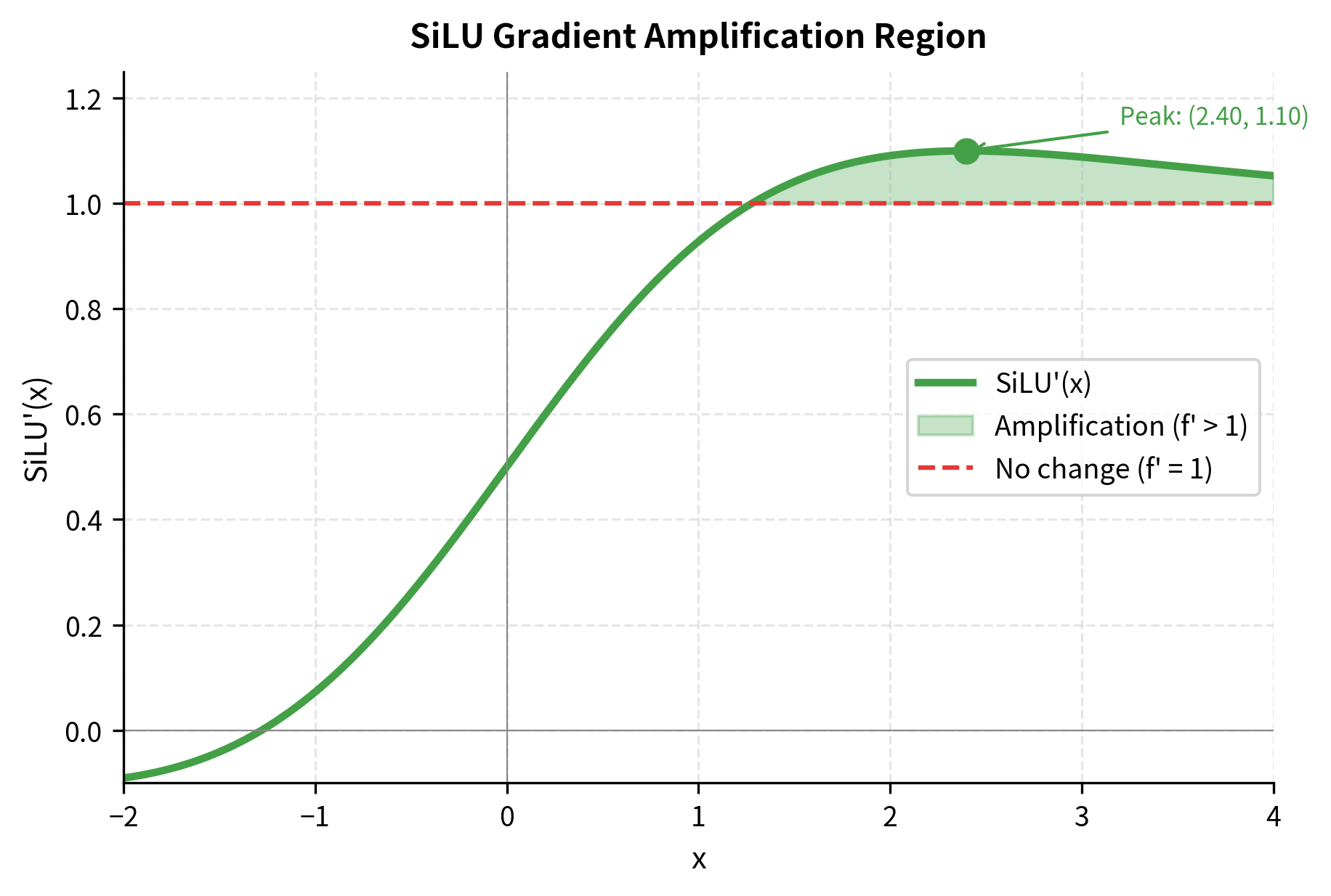
Slightly stronger gradients: SiLU's derivative can exceed 1 (peaking around 1.1 near ), which may help gradient flow in very deep networks. GELU's derivative is bounded between 0 and 1.
-
Empirical performance: In large-scale experiments at the scale of modern LLMs, SiLU consistently matches or slightly outperforms GELU for autoregressive language modeling. The differences are small but measurable.
-
Pairing with gated linear units: Modern architectures like LLaMA use SiLU specifically within gated linear unit (GLU) variants, where the activation's properties interact with the gating mechanism. We'll explore this in the next chapter.
Activation Function Comparison
With all three activations implemented, let's visualize them together to understand their relationships and differences:
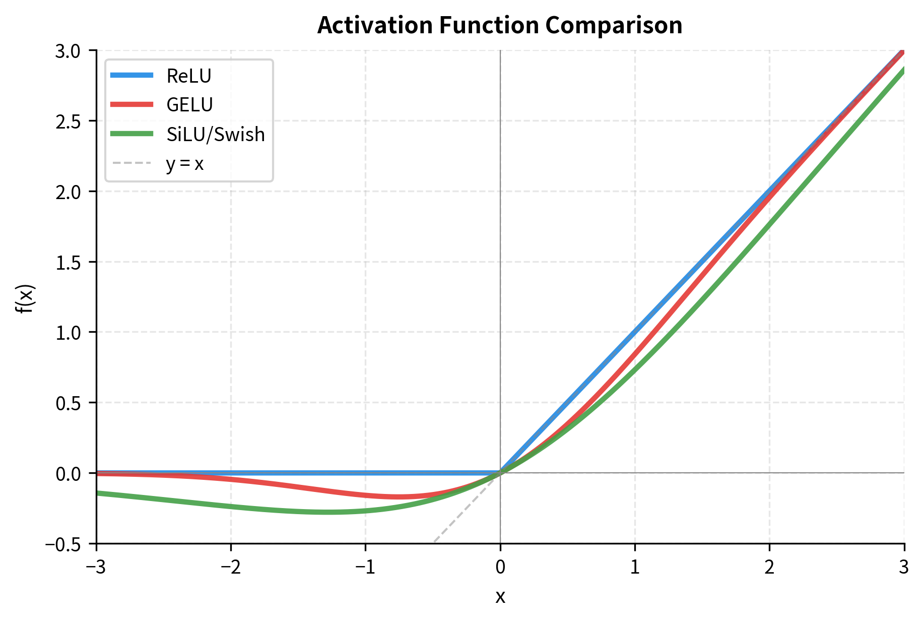
The three functions converge for large positive inputs, approaching the identity function. They also converge for large negative inputs, approaching zero. The critical differences are in the transition region around zero, where:
- ReLU has a sharp corner with discontinuous derivative
- GELU has a smooth transition with a slight negative dip (minimum at )
- SiLU has a smooth transition with a deeper negative dip (minimum at )
Let's also compare the derivatives, which directly affect gradient flow during training:
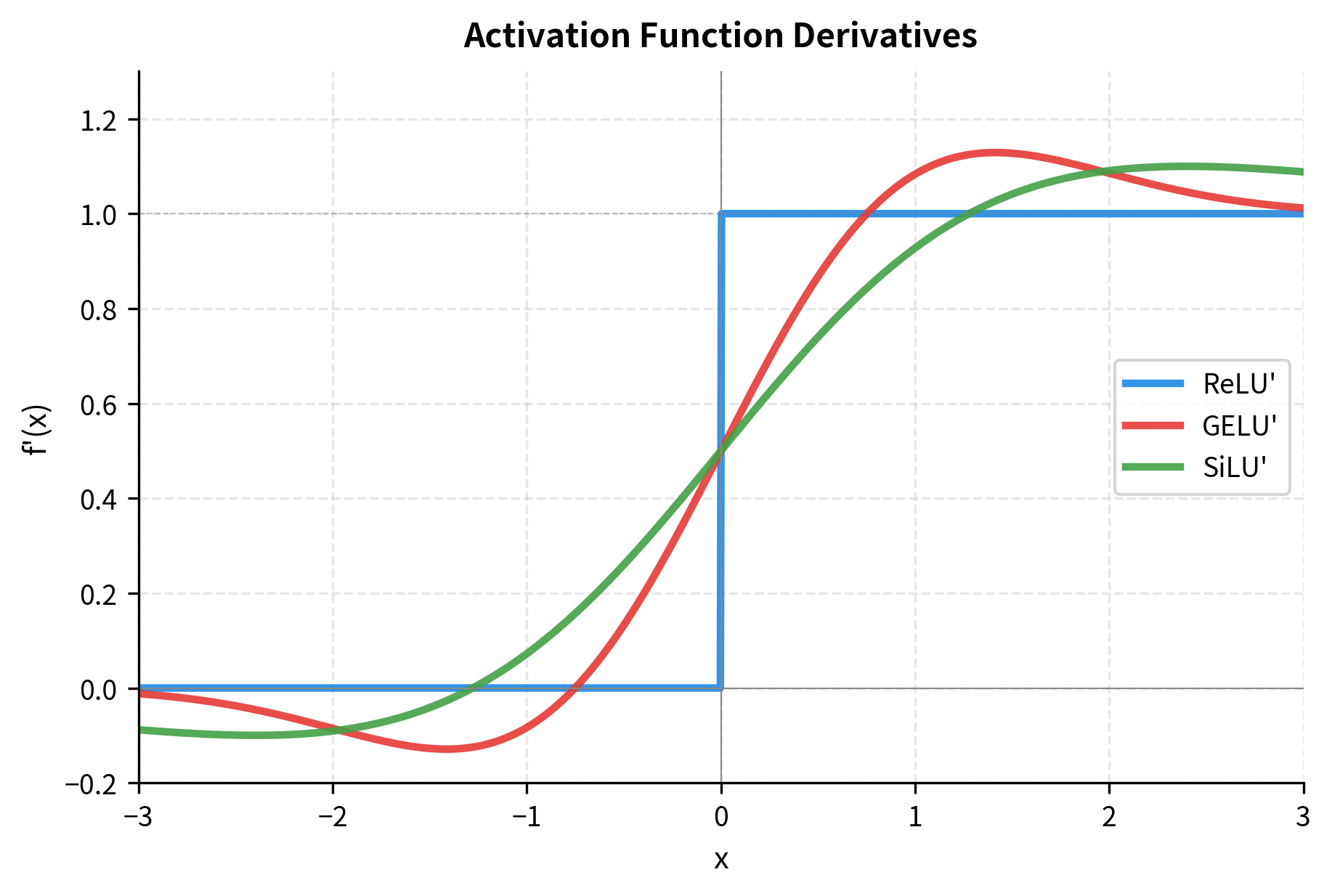
The derivative plots reveal a crucial difference: SiLU's derivative can exceed 1.0, reaching approximately 1.1 near . This means SiLU can slightly amplify gradients for certain input values, potentially helping gradient flow in very deep networks. Let's visualize where this gradient amplification occurs:
Quantitative Comparison
Let's compute specific properties that affect neural network behavior:
Key observations from this analysis:
-
Minimum value: ReLU never goes negative (by definition). GELU's dip is mild (-0.17), while SiLU dips deeper (-0.28). These negative values can help with regularization but also introduce potential instabilities.
-
Sparsity: All three create some degree of sparsity (outputs near zero), but ReLU is the most sparse for normally distributed inputs. This sparsity can aid interpretability and efficiency.
-
Linearity: All three are highly linear for positive inputs (correlation > 0.999 with ), which helps preserve signal magnitude through deep networks.
The Negative Dip: Feature or Bug?
GELU and SiLU's negative regions deserve closer examination. For certain negative inputs, these activations produce negative outputs rather than zero. This seems counterintuitive: why would we want activations to sometimes invert their input's sign?
The negative dip serves as a form of implicit regularization. Consider what happens during training: inputs that land in the dip region (roughly for GELU) get attenuated but not eliminated. This "soft gating" provides a richer gradient signal than ReLU's hard zero, potentially helping the network escape local minima.
The magnitude of the dip matters for training dynamics. A deeper dip (SiLU) means stronger negative signals for moderately negative inputs, which could either help or hurt depending on the task. Empirically, both work well, with the choice often coming down to which pairs better with other architectural decisions (like gated linear units).
Activation Functions in Practice
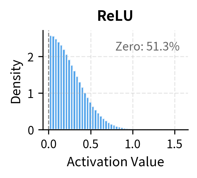
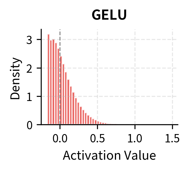
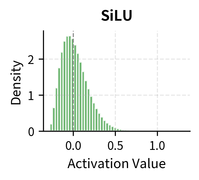
Let's simulate how these activations behave in an actual FFN layer, processing typical transformer hidden states:
The statistics reveal important differences. ReLU creates the sparsest representations (50% of values near zero) and has no negative outputs. GELU and SiLU have less sparsity and a small fraction of negative outputs. The mean activation is higher for the smooth activations because they don't hard-threshold negative inputs to zero.
Computational Efficiency
Activation function speed matters at scale. When processing billions of tokens through trillion-parameter models, even small differences in activation computation time accumulate. Let's benchmark our implementations:
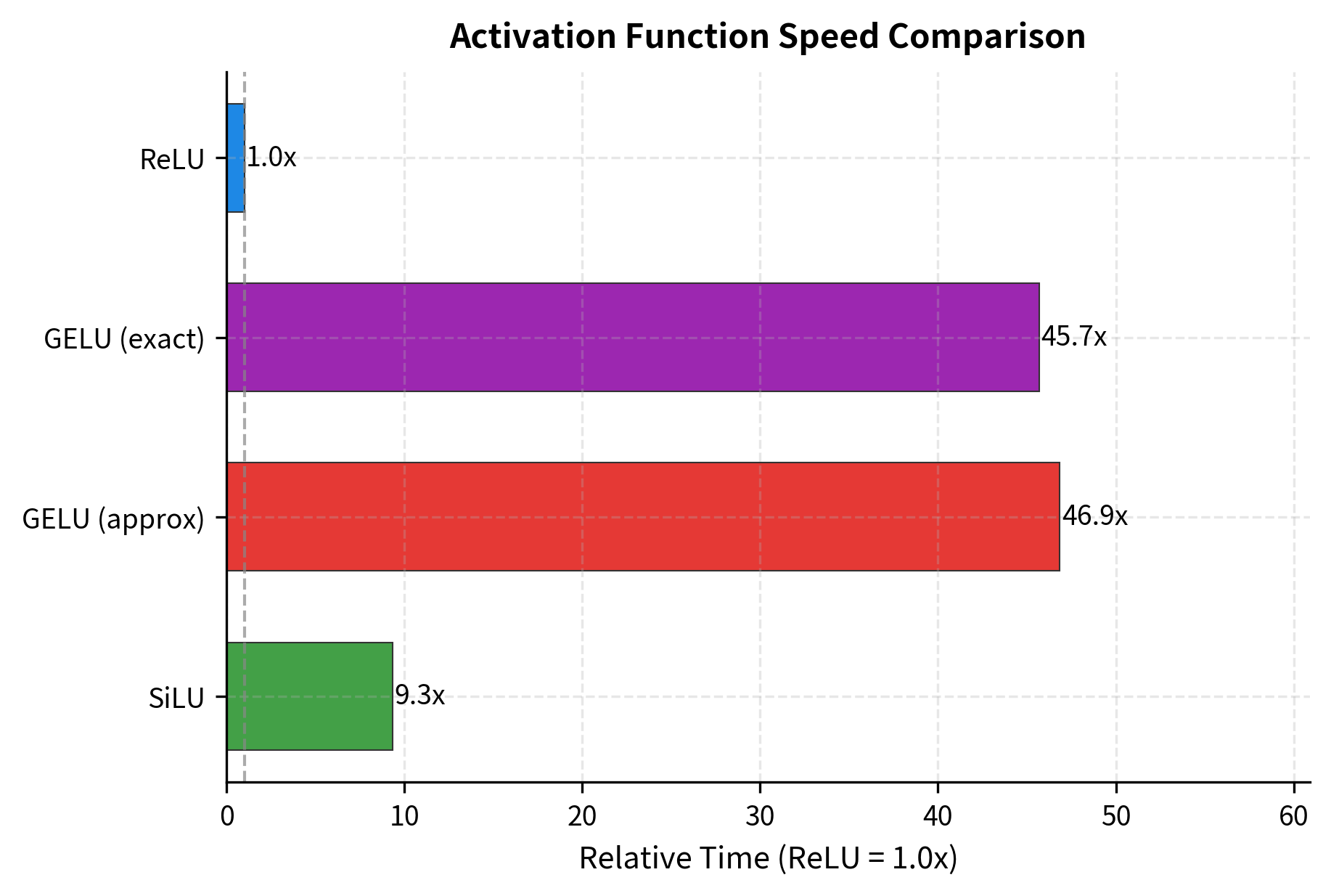
ReLU is fastest because it's just a comparison operation. The exact GELU using erf is slowest. The GELU tanh approximation is faster than exact GELU but still slower than SiLU. SiLU is relatively fast because sigmoid has efficient implementations on most hardware.
In practice, these differences are often dwarfed by memory bandwidth limitations and matrix multiplication costs. The activation function typically accounts for less than 1% of total FFN compute time. Still, at sufficient scale, even small improvements matter.
Which Activation Should You Use?
The choice of activation function depends on your model architecture and use case. Here's a practical guide:
Use ReLU when:
- You need maximum computational efficiency and simplicity
- You're building a custom architecture and want a well-understood baseline
- Your model is small enough that the dead neuron problem is manageable
- You're working with older codebases or frameworks that expect ReLU
Use GELU when:
- You're building an encoder model (BERT, RoBERTa, ELECTRA style)
- You want compatibility with pretrained encoder models
- You prioritize smooth gradients over computational efficiency
- You're fine-tuning an existing GELU-based model
Use SiLU when:
- You're building a decoder model (GPT, LLaMA, Mistral style)
- You're using gated linear units (SwiGLU, GeGLU) in your FFN
- You want the slight performance edge that modern LLMs have demonstrated
- You need a smooth activation but prefer simpler computation than GELU
The empirical differences between GELU and SiLU are often small. Unless you're training at massive scale where every fraction of a percent matters, either smooth activation will likely work well. The more important choice is between ReLU (with its dead neuron risk) and the smooth alternatives.
Implementation: Configurable Activation Module
Let's create a configurable activation function module that supports all three options, following patterns used in modern transformer libraries:
Limitations and Impact
The choice of activation function in transformer FFNs has subtle but measurable effects on model behavior. While the differences between GELU and SiLU are often small in benchmarks, they compound across billions of forward passes during training.
One underappreciated limitation is numerical stability. GELU's error function and SiLU's exponential can both produce numerical issues at extreme input values. Production implementations include clipping (as we did for sigmoid) and sometimes use mixed-precision computation to balance speed and stability.
Another consideration is hardware optimization. Modern GPUs and TPUs have specialized circuits for certain operations. The sigmoid function in SiLU benefits from this optimization on many accelerators. GELU's error function is less universally optimized, which partly explains the trend toward SiLU in recent models despite GELU's theoretical elegance.
The impact of activation functions extends beyond raw performance. The smooth gradients of GELU and SiLU allow for more stable training at large batch sizes and high learning rates. This was crucial for scaling transformers to billions of parameters, where training instability becomes a serious concern.
Looking forward, activation functions continue to evolve. Gated linear units (covered in the next chapter) combine activation functions with multiplicative gating, creating even richer nonlinearities. The field hasn't settled on a final answer, and future architectures may introduce entirely new activation functions that further improve on the current options.
Summary
Activation functions inject nonlinearity into the feed-forward network, enabling transformers to learn complex functions of language. This chapter traced the evolution from ReLU to GELU to SiLU, examining the mathematical properties that make each suitable for different contexts.
Key takeaways:
-
ReLU () is the simplest activation, with zero computation cost beyond a comparison. Its sharp corner creates sparse representations but risks "dead neurons" that stop learning entirely. ReLU was used in the original transformer but has been largely superseded in modern architectures.
-
GELU () smoothly gates inputs by their Gaussian CDF values. The result is a differentiable, non-monotonic function with a slight negative dip around . GELU became the standard for encoder models (BERT, RoBERTa) and remains widely used.
-
SiLU/Swish () multiplies inputs by their sigmoid values. Like GELU, it's smooth and non-monotonic, but with a deeper negative dip and slightly simpler computation. SiLU has become the standard for decoder models (LLaMA, Mistral, GPT-NeoX).
-
Practical choice: The differences between GELU and SiLU are often small in practice. Choose based on your model family (encoder vs. decoder), compatibility with pretrained models, or specific architectural requirements like gated linear units.
-
Computational efficiency: ReLU is fastest, followed by SiLU, then GELU approximation, then exact GELU. However, activation computation is typically less than 1% of total FFN time, so speed rarely drives the choice.
The next chapter examines gated linear units (GLUs), which combine activation functions with multiplicative gating to create even more expressive FFN architectures. Variants like SwiGLU and GeGLU have become standard in state-of-the-art models like LLaMA and PaLM.
Key Parameters
When configuring activation functions for transformer FFNs, these parameters and choices affect model behavior:
-
activation_type: The activation function to use. Common options are
"relu","gelu","gelu_approximate", and"silu". Choose based on your model architecture: GELU for encoder models (BERT-style), SiLU for decoder models (LLaMA-style), or ReLU for maximum simplicity and speed. -
approximate (for GELU): Whether to use the tanh approximation instead of the exact error function. The approximation is faster on most hardware and introduces negligible error (< 0.005 maximum). Most production systems use the approximation.
-
inplace (framework-specific): Some frameworks allow in-place activation to reduce memory usage. This modifies the input tensor directly rather than creating a new output tensor. Use with caution, as it can cause issues with gradient computation if the original values are needed.
-
numerical clipping (for SiLU/sigmoid): Input values should be clipped to prevent overflow in the exponential function. A range of is typical. Most deep learning frameworks handle this automatically, but custom implementations should include explicit clipping.
-
dtype considerations: Activation functions behave differently at different precisions. At float16 or bfloat16, the dynamic range is limited, which can cause issues with the exponential in SiLU or the error function in GELU. Mixed-precision training typically keeps activations in higher precision for stability.
Quiz
Ready to test your understanding? Take this quick quiz to reinforce what you've learned about activation functions in transformer feed-forward networks.

Comments