

Deep dive into Mistral 7B's architectural innovations including sliding window attention, grouped query attention, and rolling buffer KV cache. Learn how these techniques achieve LLaMA 2 13B performance with half the parameters.

This article is part of the free-to-read Language AI Handbook
Choose your expertise level to adjust how many terms are explained. Beginners see more tooltips, experts see fewer to maintain reading flow. Hover over underlined terms for instant definitions.
Mistral Architecture
When Mistral AI released their 7B parameter model in September 2023, it achieved something remarkable: matching or exceeding the performance of LLaMA 2 13B on most benchmarks while using nearly half the parameters. This wasn't magic. It was the result of carefully chosen architectural innovations that improve efficiency without sacrificing capability. The most significant of these is sliding window attention, a technique that limits the computational burden of attention while preserving the model's ability to reason over long contexts.
This chapter dissects the Mistral architecture, examining how it builds on the LLaMA foundation while introducing key modifications that boost efficiency. We'll implement sliding window attention from scratch, visualize how it differs from full attention, and understand why Mistral's design choices have made it one of the most influential open-weight models in the field.
Architectural Foundation
Mistral 7B inherits the core structure of LLaMA while introducing targeted improvements. Understanding these changes requires first recognizing what stays the same: Mistral uses a decoder-only transformer with RMSNorm for layer normalization, SwiGLU for the feed-forward network, and rotary positional embeddings (RoPE) for encoding position information. These components, proven effective in LLaMA, form the foundation upon which Mistral builds.
The key architectural parameters for Mistral 7B are:
- Hidden dimension: 4096
- Number of layers: 32
- Number of attention heads: 32
- Number of KV heads: 8 (grouped query attention)
- Feed-forward hidden dimension: 14336
- Vocabulary size: 32000
- Context length: 8192 tokens (sliding window of 4096)
- Total parameters: 7.3 billion
Three innovations distinguish Mistral from its predecessors: sliding window attention (SWA), rolling buffer KV cache, and pre-fill chunking. Together, these enable efficient processing of long sequences while maintaining strong performance.
The configuration reveals Mistral's efficiency-focused design. The 8 KV heads (compared to 32 query heads) indicate grouped query attention, while the 4096-token sliding window enables the model to handle 8K context lengths without quadratic memory growth.
Sliding Window Attention
To understand sliding window attention, we need to first appreciate the problem it solves. Standard self-attention allows every token to attend to every other token. This seems natural: when predicting the next word, shouldn't the model consider the entire context? The answer is yes, in principle. But the computational reality tells a different story.
The Quadratic Problem
Consider what happens when you compute attention. For each token in your sequence, you calculate a score against every other token. With tokens, that's scores per token, and tokens total, giving scores. Store these in memory, and you need space proportional to . Compute them, and you need operations proportional to .
This quadratic scaling creates a harsh reality:
| Sequence Length | Attention Scores | Growth Factor |
|---|---|---|
| 1,024 tokens | ~1 million | 1x |
| 4,096 tokens | ~17 million | 16x |
| 16,384 tokens | ~268 million | 256x |
Doubling the sequence length quadruples both memory and compute. By the time you reach 16K tokens, a common context length for modern models, you're dealing with hundreds of millions of attention scores per layer. Multiply by 32 layers and the numbers add up quickly.
The Sliding Window Insight
Mistral's solution starts with a simple observation: in practice, tokens rarely need to attend to the entire preceding context with equal importance. Recent tokens matter more than distant ones for most language patterns. What if we formalized this intuition and restricted attention to only the most recent tokens?
This is exactly what sliding window attention does. Instead of allowing token to attend to all tokens from 0 to , we restrict it to a fixed window of size . Token can only attend to tokens in positions through , a span of at most tokens.
Think of it like looking through a sliding window that moves along with your position in the sequence. Early in the sequence, when you're at position 3, you might see positions 0, 1, 2, and 3. Later, at position 1000, you see positions 997, 998, 999, and 1000. The window always contains the same number of tokens (or fewer, at the start), regardless of how long the sequence grows.
From Intuition to Formula
Let's formalize this sliding window mathematically. We need a mask that tells the attention mechanism which positions are allowed (within the window) and which are forbidden (outside the window or in the future).
The attention mask determines whether query position can attend to key position :
Let's unpack each component:
- : the query position, meaning the token that's "asking" for information
- : the key position, meaning the token that might provide information
- : the window size (4096 for Mistral 7B)
- : the leftmost position in the window, clamped to 0 for early tokens
- The condition : defines the valid window, positions can attend to
The mask values themselves serve a specific purpose in the attention computation:
- : When added to attention scores, leaves them unchanged, allowing attention
- : When added to attention scores, makes them negative infinity. After softmax, , completely blocking attention
Why this particular formulation? The answer lies in how attention scores become attention weights. Raw scores pass through softmax, which exponentiates each score. By adding to forbidden positions, we ensure their exponentiated values are exactly zero, not just small. This creates a hard boundary that the model cannot violate.
Complexity Transformation
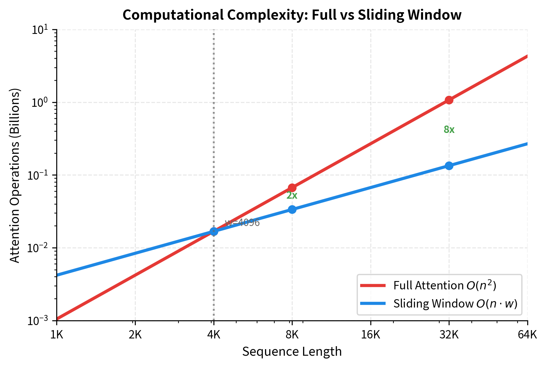
The power of sliding window attention becomes clear when we analyze its complexity. With full attention, each of tokens computes scores against all tokens, giving operations. With sliding window attention, each of tokens computes scores against only tokens, giving operations.
When is fixed (4096 for Mistral), this becomes : linear in sequence length. The difference is significant:
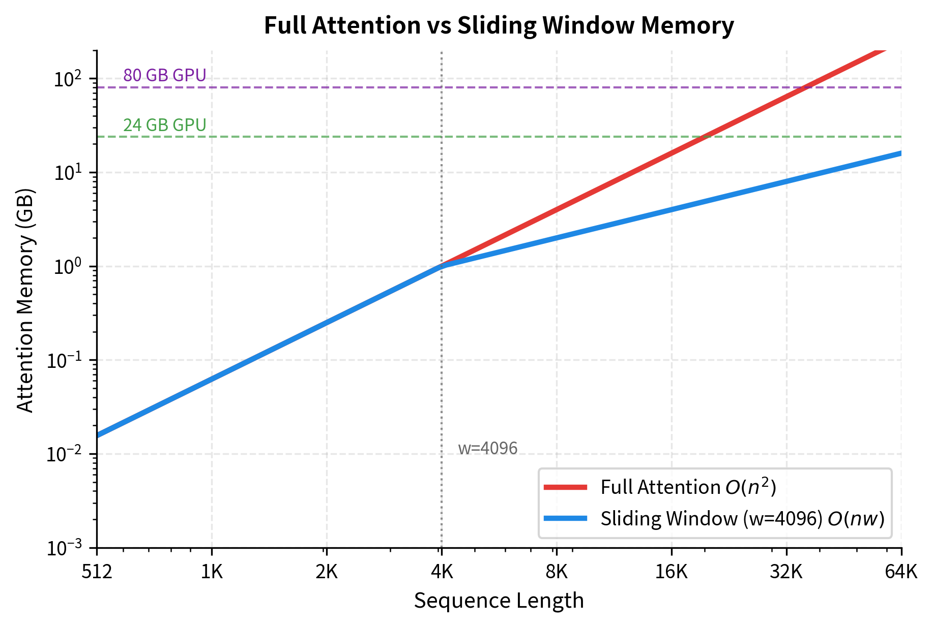
- Full attention at 32K tokens: billion scores
- Sliding window at 32K tokens: million scores
That's an 8x reduction at 32K tokens, and the gap widens as sequences grow longer.
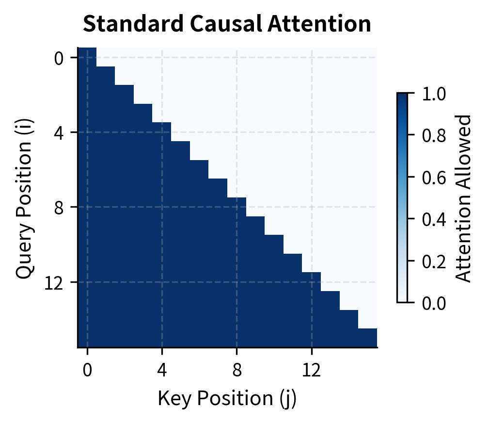
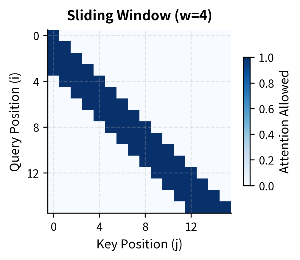
The visual difference is clear. Standard causal attention fills the entire lower triangle, meaning late tokens must process attention scores for all preceding tokens. Sliding window attention creates a narrow band along the diagonal, greatly reducing the number of computations.
Information Flow Across Layers
A natural concern arises: if each token can only see tokens back, how does the model capture long-range dependencies? If the sliding window is 4096 tokens, can a token at position 8000 ever learn anything from a token at position 100?
The answer is yes, and understanding why requires thinking about how information propagates through stacked transformer layers.
The Layered Propagation Mechanism
Consider a concrete example. At layer 1, token 8000 can directly attend to tokens 3905 through 8000 (a window of 4096 positions). It cannot see token 100 directly. But here's the key insight: token 3905 at layer 1 could see tokens 0 through 3905. When token 8000 attends to token 3905 at layer 2, it's attending to a representation that already contains information from the beginning of the sequence.
Each layer extends the reach:
- Layer 1: Token sees positions , a direct window of tokens
- Layer 2: Token attends to tokens that themselves saw tokens back, extending indirect reach to
- Layer : Information can travel up to positions through layered propagation
This gives us the receptive field formula:
where:
- : the receptive field at layer , measuring how far back information can theoretically travel
- : the layer number (1 to )
- : the sliding window size
Applying the Formula to Mistral
For Mistral 7B with layers and :
This theoretical receptive field of 131K tokens vastly exceeds Mistral's 8K context length. Even at layer 2, the receptive field is tokens, covering the entire context window.
This analysis reveals an important design choice: Mistral's window size and layer count are calibrated so that the receptive field exceeds the context length early in the network. By layer 2, any token can (indirectly) access information from any other token in the context.
The Trade-off: Direct vs Indirect Access
While the receptive field ensures information can flow across the entire context, there's a qualitative difference between direct and indirect access. When token 8000 directly attends to token 7999, it sees that token's representation with full fidelity. When it indirectly accesses token 100 through layered propagation, the information has passed through multiple aggregation steps, potentially becoming more diffuse.
For tasks requiring precise retrieval of specific early tokens, this indirect propagation may be less effective than full attention. But for most language modeling tasks, where context builds gradually and recent tokens matter most, the sliding window provides an excellent trade-off between efficiency and capability.
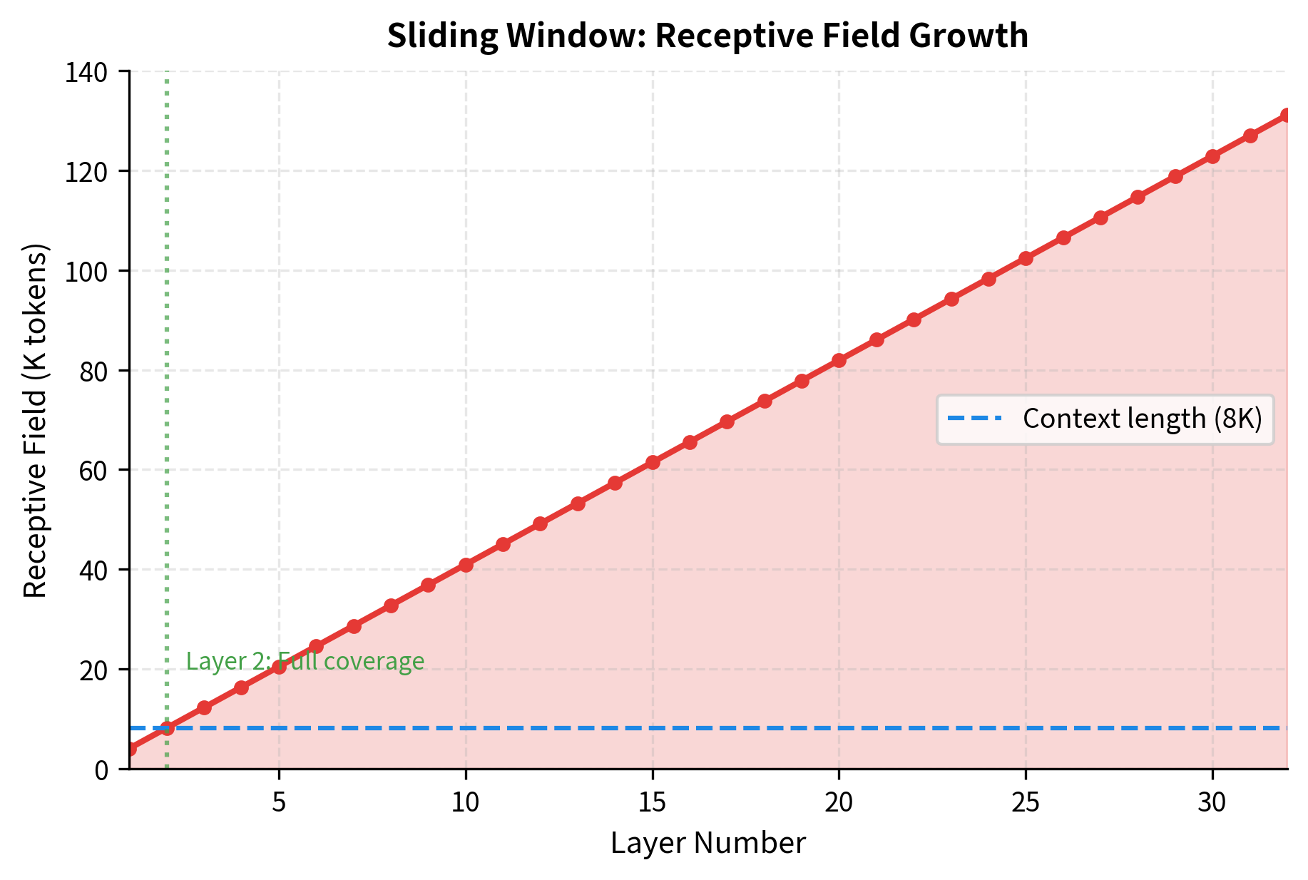
The visualization shows that by layer 2, the receptive field already exceeds the 8K context length. This means that even though individual attention operations are local, the overall architecture can still capture dependencies spanning the entire input.
Memory and Compute Savings
Understanding the theory of sliding window attention is valuable, but the practical impact is what matters for deployment. Let's derive exactly how much memory and compute we save, starting from first principles.
Deriving the Memory Formulas
The attention mechanism computes a score for each query-key pair. With query positions and key positions, we have scores to store. Each attention head maintains its own score matrix, and each score requires storage space determined by the numerical precision.
For full attention, the memory required is:
For sliding window attention, each query position only attends to key positions. When the sequence is shorter than the window (), we still compute scores per query. When the sequence exceeds the window (), we compute exactly scores per query:
Let's define each variable precisely:
- : total memory in bytes for all attention score matrices
- : sequence length (number of tokens)
- : sliding window size (4096 for Mistral)
- : number of attention heads (32 for Mistral)
- : bytes per element (2 for fp16, 4 for fp32)
The Crossover Point
The formulas reveal a key insight: the two methods behave identically when . Both compute the same attention matrix because the window hasn't started to "slide" yet. The divergence occurs when :
- Full attention: Memory grows as , accelerating as sequences lengthen
- Sliding window: Memory grows as , which is linear in since is fixed
For Mistral with , the crossover happens at 4096 tokens. Below this, both methods are equivalent. Above this, sliding window provides increasing savings:
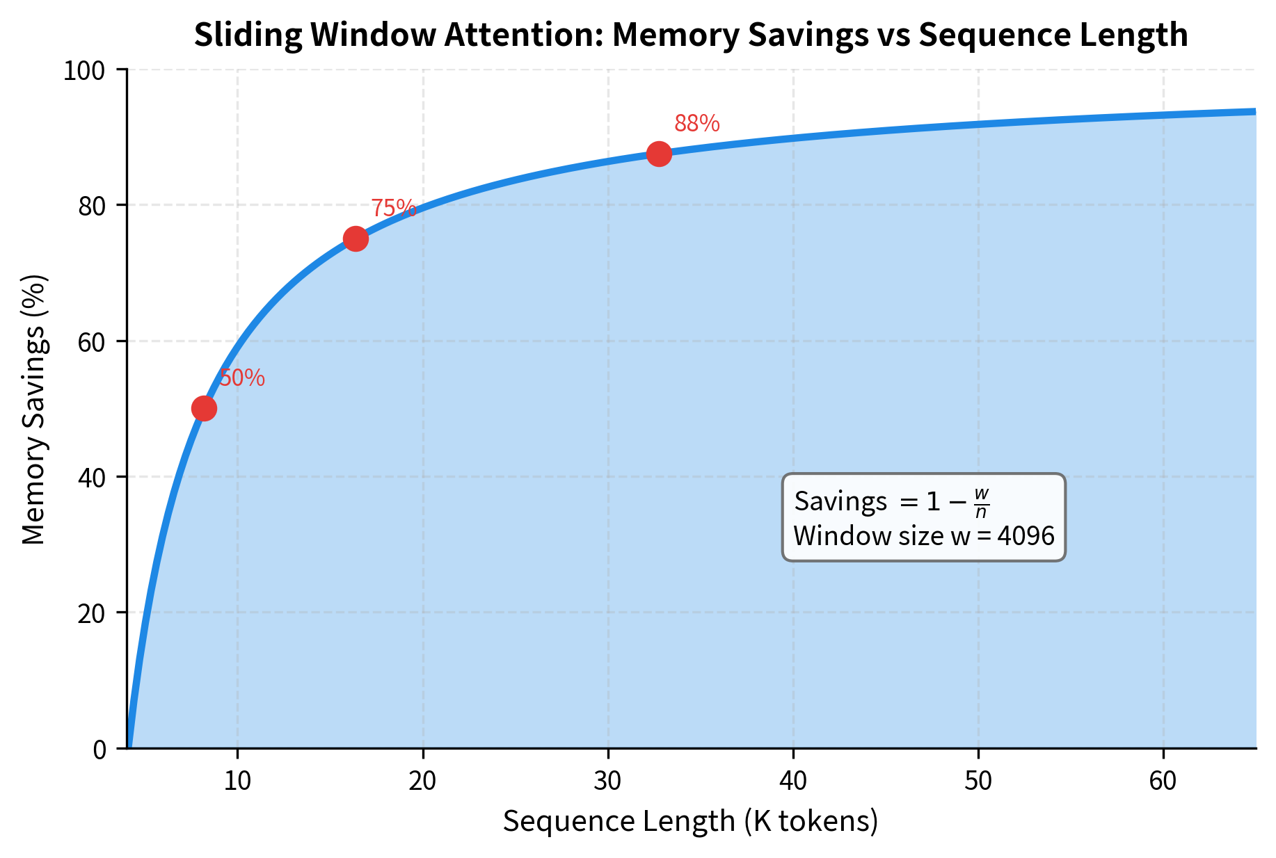
- At : Sliding window uses the memory (50% savings)
- At : Sliding window uses the memory (87.5% savings)
The savings percentage follows a simple formula: when . As sequences grow longer, the savings approach 100%.
Quantifying the Savings
Let's compute concrete memory numbers for Mistral's configuration:
At the 8K context length that Mistral supports, sliding window attention uses exactly half the memory of full attention. At 32K tokens, the savings exceed 87%. These memory reductions directly translate to the ability to process longer sequences or use larger batch sizes.
The crossover point at the window size (4096) matters. Below this threshold, both methods use similar memory because sequences are shorter than the window. Beyond this point, sliding window attention's linear scaling provides increasing advantages.
Rolling Buffer KV Cache
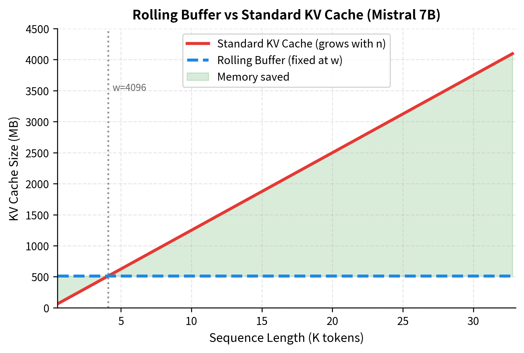
During autoregressive generation, transformers cache the key and value projections of previous tokens to avoid redundant computation. In standard transformers, this KV cache grows linearly with sequence length, eventually consuming significant memory for long generations.
Mistral implements a rolling buffer KV cache that exploits sliding window attention. Since tokens beyond the window boundary will never be attended to again, their cached keys and values can be safely discarded. The cache maintains only the most recent positions, using modular indexing to overwrite old entries.
The rolling buffer ensures that memory usage remains constant regardless of how many tokens are generated. For a 32-layer Mistral model with 8 KV heads per layer, the total cache memory is fixed at:
where:
- : total memory in bytes for the KV cache
- : factor accounting for storing both keys and values (each cached position stores one K vector and one V vector)
- : number of transformer layers (32 for Mistral 7B), since each layer maintains its own KV cache
- : sliding window size (4096 for Mistral), the maximum number of positions stored
- : number of key-value heads per layer (8 for Mistral 7B with GQA)
- : dimension of each head, computed as where and , giving
- : bytes per element (2 for fp16, 4 for fp32)
For Mistral 7B with fp16 precision, the fixed cache size is:
This fixed 512 MB footprint contrasts sharply with standard transformers, where the cache grows linearly with sequence length and could reach several gigabytes for long generations.
The fixed memory footprint is valuable for deployment scenarios where memory budgets are tight and generation lengths are unpredictable.
Grouped Query Attention
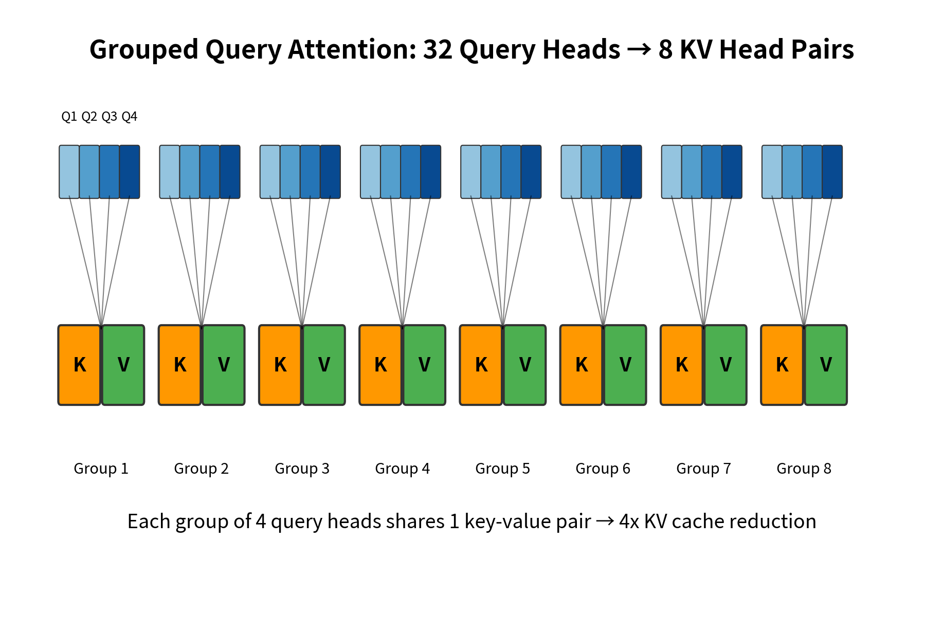
Mistral employs grouped query attention (GQA), which reduces the number of key-value heads relative to query heads. Instead of the standard multi-head attention where each query head has its own key-value pair, GQA groups multiple query heads to share the same key-value heads.
GQA is a memory-bandwidth optimization where query heads share key-value heads, with being a multiple of . In this notation:
- : number of query heads (32 for Mistral)
- : number of key-value heads (8 for Mistral)
- : the grouping ratio (4 for Mistral, meaning 4 query heads share each KV head)
This reduces KV cache size by a factor of while maintaining most of the representational capacity of full multi-head attention.
For Mistral 7B:
- Query heads: 32
- KV heads: 8
- Ratio: 4 query heads share each KV head
This means the KV cache is 4x smaller than it would be with standard multi-head attention, directly improving inference throughput by reducing memory bandwidth requirements.
The combination of GQA and the rolling buffer creates substantial memory savings. With 8 KV heads instead of 32, and a fixed window size instead of growing with sequence length, Mistral's inference memory footprint remains manageable even for long-context applications.
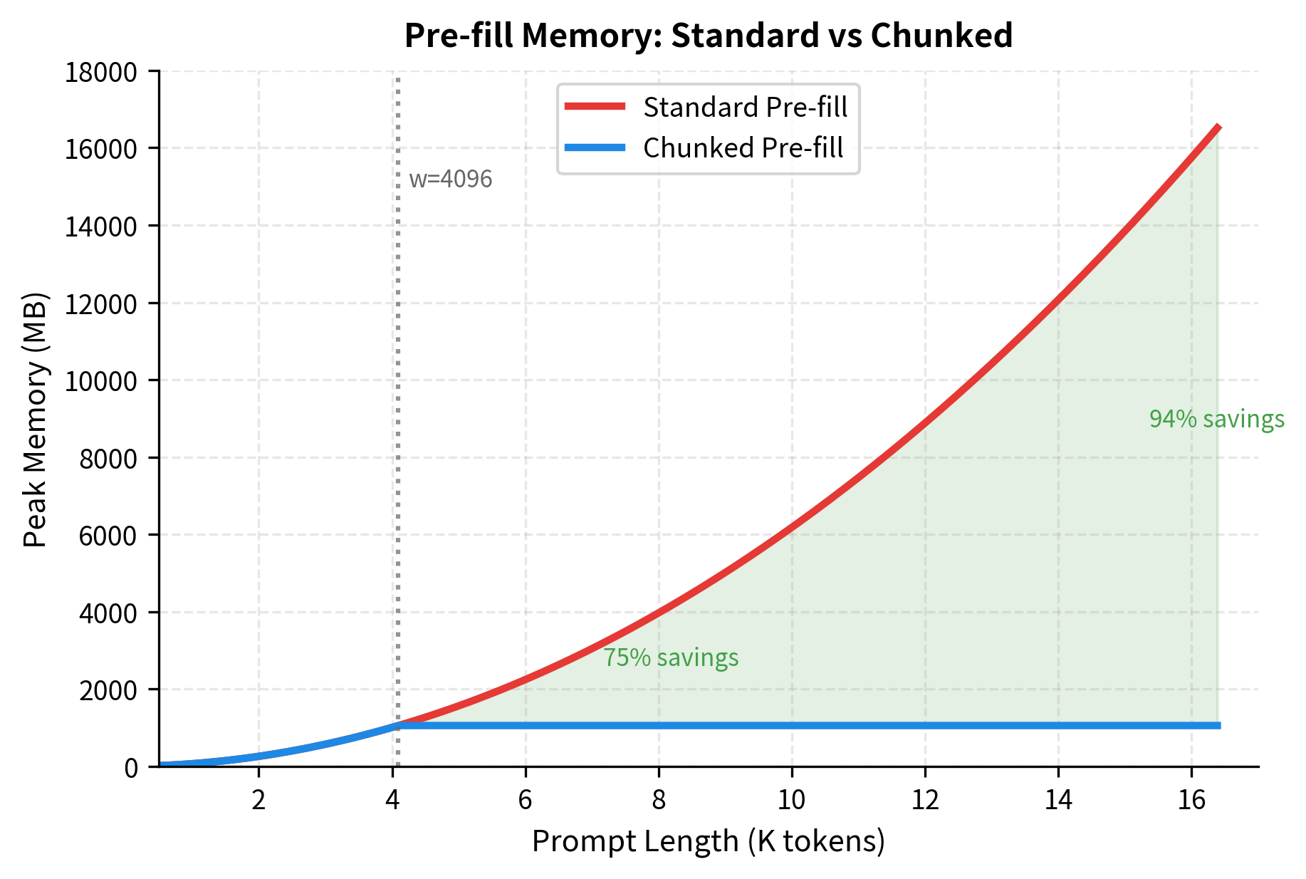
Pre-fill and Chunking
When processing a prompt before generation begins, standard transformers compute attention for all tokens at once. For long prompts, this can create memory spikes that exceed available capacity. Mistral introduces pre-fill chunking to address this.
The idea is simple: instead of processing the entire prompt in a single forward pass, split it into chunks of size (the window size). Process each chunk sequentially, using the rolling KV cache to maintain context between chunks. This bounds memory usage during pre-fill to the same level as during generation.
For an 8K token prompt, chunked pre-fill uses 75% less memory than standard pre-fill. This reduction enables processing of longer prompts on the same hardware, or processing multiple requests concurrently.
Implementation: Sliding Window Attention
Having understood the mathematics behind sliding window attention, let's implement it from scratch. Building the mechanism ourselves will solidify the concepts and reveal implementation details that matter in practice.
Step 1: Building the Attention Mask
The foundation of sliding window attention is the mask that enforces which positions can attend to which. We need to encode two constraints:
- Causal constraint: Position cannot attend to any position (no looking into the future)
- Window constraint: Position cannot attend to any position (outside the sliding window)
Both constraints translate to blocking certain positions with values:
The logic is straightforward: for each position pair , we check if is in the future () or outside the window (). If either condition is true, we block with .
Let's visualize the mask to verify it matches our expectations:
Reading this output row by row tells the story of the sliding window:
- Token 0: Can only attend to itself (the sequence just started)
- Token 1: Can attend to positions 0-1 (window not yet full)
- Token 2: Can attend to positions 0-2 (window not yet full)
- Token 3: Can attend to positions 0-3 (window now full with 4 positions)
- Token 4: The window slides! Can attend to positions 1-4, blocking position 0
- Tokens 5-7: The window continues sliding, always covering exactly 4 positions
This banded diagonal structure is what transforms quadratic complexity into linear.
Step 2: The Complete Attention Forward Pass
With the mask in place, we can implement the full sliding window attention computation. The algorithm follows the standard attention formula, but with our sliding window mask applied before softmax:
Let's walk through this implementation step by step:
-
Reshaping: We transpose from
(batch, seq, heads, dim)to(batch, heads, seq, dim)to enable batched matrix multiplication across all heads simultaneously -
Score computation: The matrix product
q @ k.Tcomputes dot products between all query-key pairs, giving raw attention scores. We scale by to prevent the softmax from becoming too peaked -
Mask application: Adding the mask ( or ) to scores enforces our sliding window constraint. Positions with will have zero attention weight after softmax
-
Stable softmax: We subtract the maximum score before exponentiating to prevent numerical overflow. This is mathematically equivalent to standard softmax but numerically stable
-
Value aggregation: The final matmul blends values according to attention weights, producing the output representation
Step 3: Testing and Visualization
Let's verify our implementation works correctly and visualize the resulting attention patterns:
The output maintains the same shape as the input queries, as expected. The attention weights tensor has shape (batch, heads, seq_len, seq_len), but only the diagonal band of width 4 contains non-zero values due to our sliding window mask.
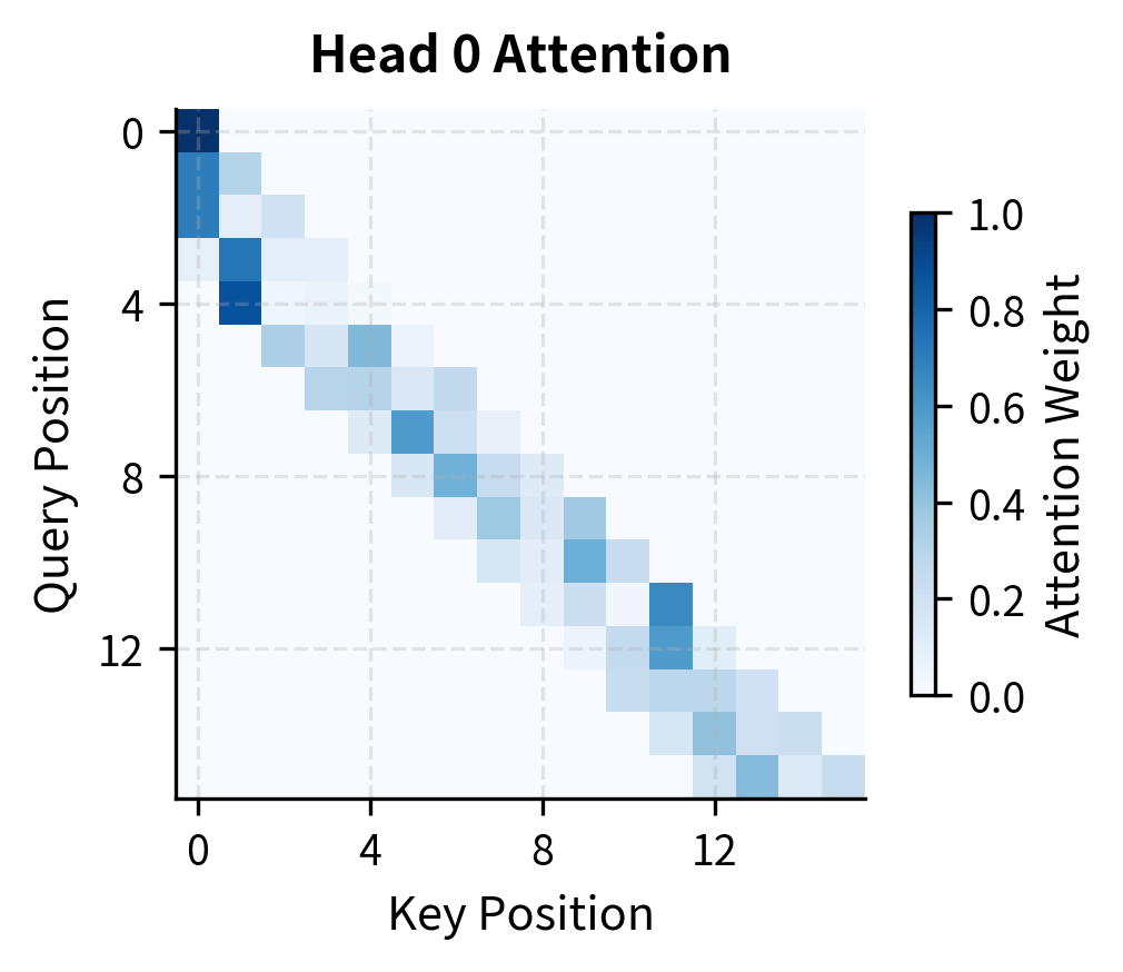
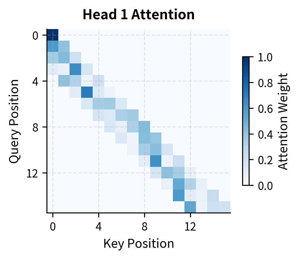
The attention heatmaps reveal several important properties of sliding window attention:
The banded structure: Each row shows attention concentrated in a diagonal band of width 4 (our window size). The strict boundaries are enforced by our mask, the positions outside the band have exactly zero attention weight.
Within-window variation: Inside the allowed window, different heads develop different patterns. Head 0 might emphasize recent positions while Head 1 focuses on slightly older ones. This diversity is valuable, different heads can specialize in different types of relationships.
Preserved expressiveness: Despite the hard constraint on which positions can be attended, the model retains full flexibility in how attention is distributed within the window. The softmax ensures weights sum to 1, but the specific allocation depends on the learned query-key interactions.
This implementation demonstrates that sliding window attention is a straightforward modification to standard attention. The only change is adding a carefully constructed mask before softmax. Everything else, the score computation, softmax normalization, and value aggregation, remains identical.
Mistral vs LLaMA: Architectural Comparison
Let's directly compare the architectural choices between Mistral 7B and LLaMA 2 7B to understand what changed:
The key differences are:
- KV heads: Mistral uses 8 KV heads (GQA) vs LLaMA's 32 (MHA), reducing KV cache by 4x
- FFN size: Mistral uses a larger intermediate dimension (14336 vs 11008), adding capacity
- Context length: Mistral supports 8K tokens vs LLaMA's 4K
- Sliding window: Mistral uses a 4096-token window, LLaMA uses full attention
These changes create a more efficient model that can handle longer contexts with less memory.
Performance Analysis
Mistral 7B achieves strong benchmark performance despite having fewer parameters than comparable models. The efficiency gains from its architectural choices translate to practical improvements in deployment.
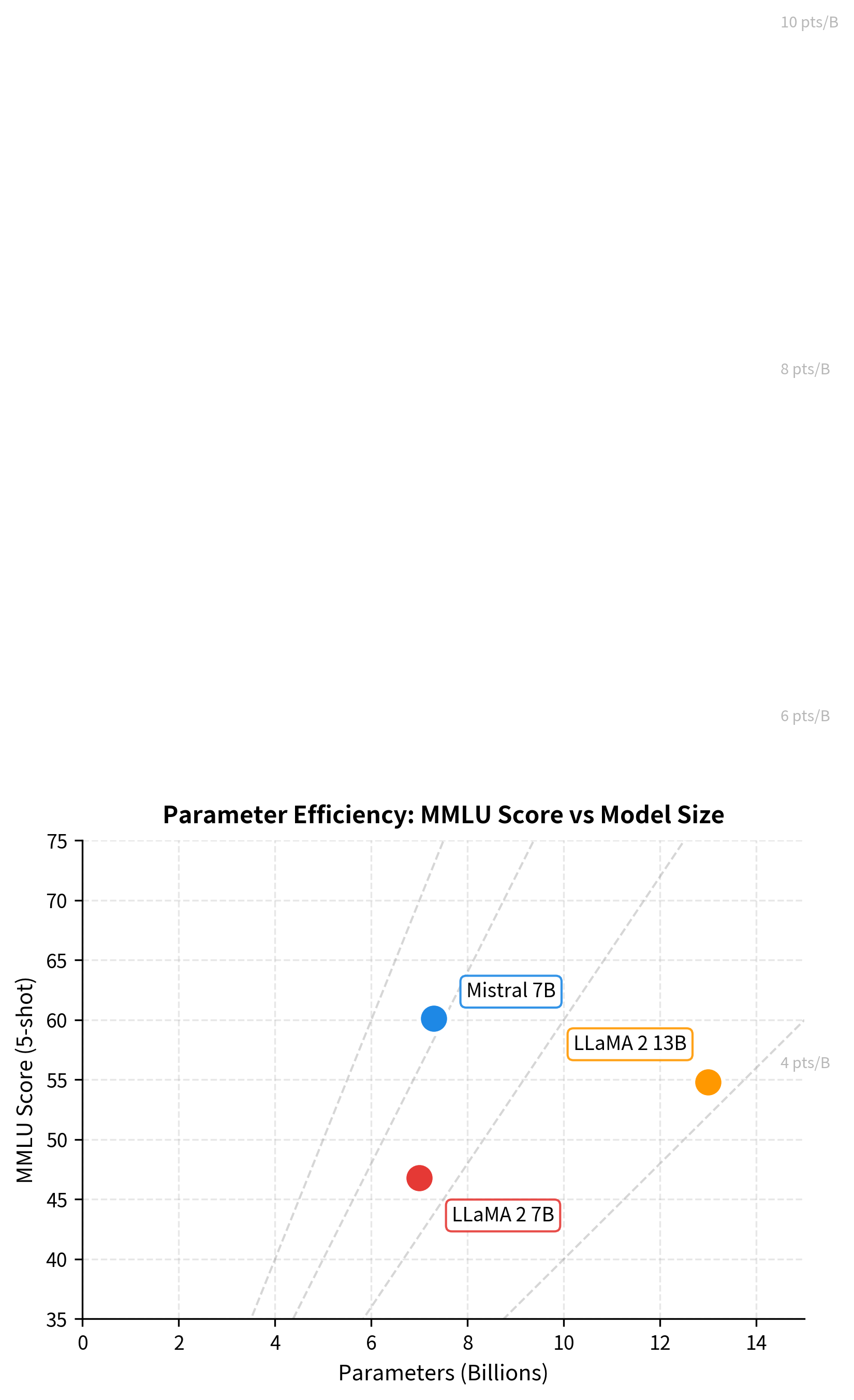
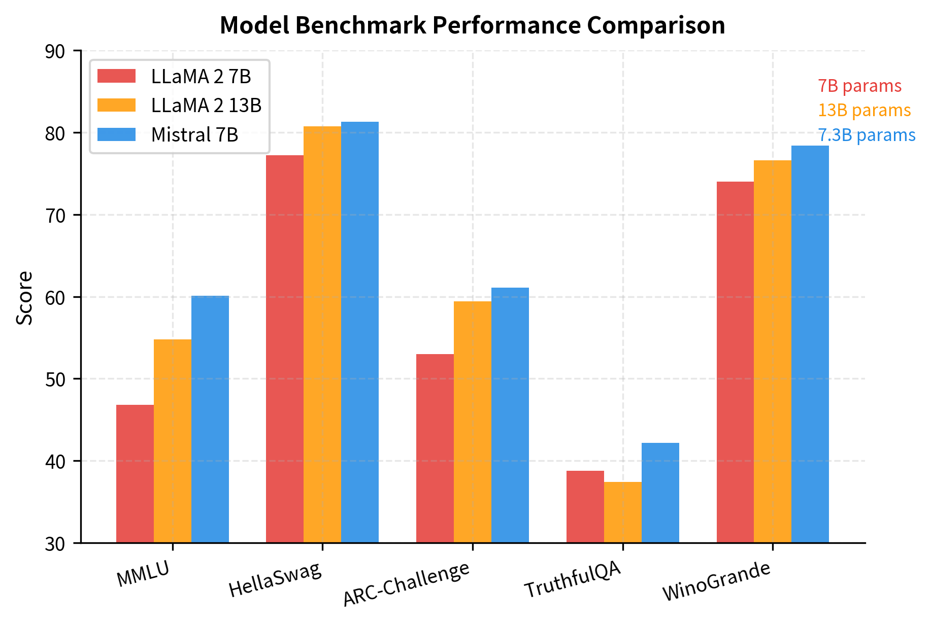
The results show that Mistral's architectural innovations enable parameter-efficient scaling. By using GQA and sliding window attention, the model frees up computational budget for a larger FFN layer and more efficient training, achieving better performance with fewer parameters.
Inference Efficiency
The practical impact of Mistral's design becomes most apparent during inference. Let's quantify the throughput improvements:
The comparison reveals Mistral's memory efficiency advantage. At 4K tokens, Mistral's KV cache is already 4x smaller due to GQA alone. At 8K tokens and beyond, the sliding window provides additional savings by capping cache growth. The total memory difference becomes substantial for long-context applications.
At 8K tokens, Mistral's KV cache is 8x smaller than LLaMA 2's would be (due to 4x from GQA and 2x from the context being capped at window size). This translates directly to higher throughput, as the memory bandwidth required to read the KV cache during each generation step is proportionally reduced.
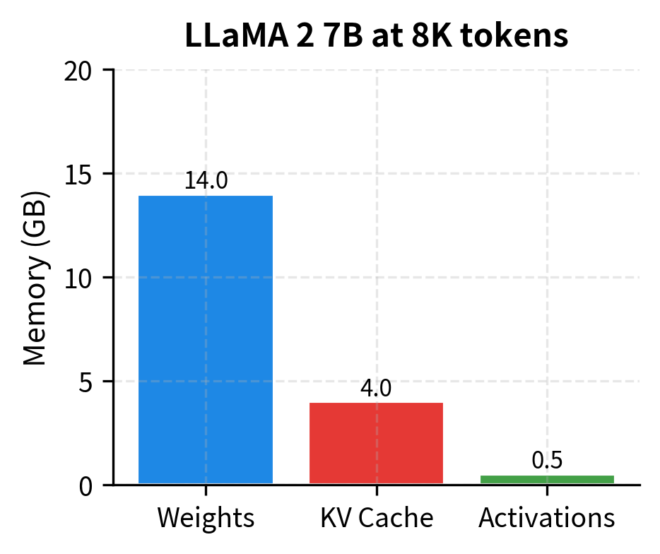
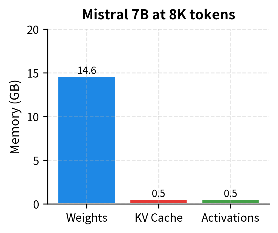
The memory breakdown visualizations show the impact of Mistral's design choices. While model weights are similar between the two architectures, the KV cache differs by nearly an order of magnitude. For LLaMA 2, the KV cache grows to dominate memory usage at long sequences. Mistral's combination of GQA (4x reduction) and rolling buffer (2x reduction at 8K context) keeps the KV cache manageable, freeing memory for larger batch sizes or longer generations.
Limitations and Considerations
While Mistral's architecture offers substantial efficiency gains, the design involves trade-offs worth understanding.
Sliding Window Limitations: The sliding window creates a hard attention cutoff. While information can propagate across layers to reach distant positions, this propagation is lossy. Information from early tokens becomes increasingly diffuse as it passes through more layers, potentially limiting performance on tasks requiring precise retrieval from early context. For tasks like long-document question answering where a specific fact from the beginning must be recalled exactly, the indirect propagation may be insufficient. In contrast, full attention can directly access any position with full fidelity.
GQA Trade-offs: Reducing KV heads from 32 to 8 means less independent key-value representations. While empirically this has minimal impact on most benchmarks, certain tasks that benefit from diverse attention patterns may see degradation. This trade-off matters most for tasks requiring fine-grained distinctions in how different query heads interpret the same input.
Pre-fill Chunking Overhead: Processing prompts in chunks requires sequential processing where parallel processing would otherwise be possible. For batch inference with many short prompts, this overhead can reduce throughput compared to processing all prompts simultaneously. The benefit only manifests for long individual sequences.
Rolling Buffer Complexity: The rolling buffer KV cache requires careful index management and can complicate certain inference optimizations. Speculative decoding and other advanced generation techniques may require modifications to work correctly with the circular buffer structure.
Despite these considerations, Mistral's design represents a compelling efficiency-capability trade-off that has proven effective across a wide range of applications. The architecture has influenced subsequent models and established sliding window attention as a viable approach for long-context language modeling.
Summary
Mistral 7B demonstrates that thoughtful architectural choices can achieve strong performance with fewer resources. The key innovations are:
-
Sliding Window Attention: Limits attention to the most recent tokens, reducing complexity from to , where is sequence length and is the fixed window size. Information propagates across layers to effectively extend the receptive field to tokens.
-
Rolling Buffer KV Cache: Stores only the most recent window of key-value pairs, keeping memory constant during generation regardless of sequence length. Combined with GQA (8 KV heads instead of 32), this reduces KV cache memory by 16x compared to full attention with standard MHA (4x from GQA, 4x from window vs full context for 16K sequences).
-
Grouped Query Attention: Four query heads share each KV head pair, reducing KV cache size by 4x while maintaining expressive capacity through independent query representations.
-
Pre-fill Chunking: Processes long prompts in window-sized chunks to bound peak memory, enabling longer context lengths on memory-constrained hardware.
These innovations work together to create a model that outperforms LLaMA 2 13B while using 44% fewer parameters. The efficiency gains don't come at the cost of capability. Instead, they free up resources that can be allocated to other components like a larger FFN layer.
The Mistral architecture has influenced the design of subsequent models and established that efficiency and performance can advance together. Sliding window attention, in particular, has become a common technique for extending context length without quadratic memory growth.
Key Parameters
The following parameters control Mistral's efficiency-capability trade-offs:
-
sliding_window(int, default=4096): The number of previous tokens each position can attend to. Larger values provide more direct context access but increase memory usage linearly. Mistral uses 4096, which balances efficiency with sufficient local context. For tasks requiring precise long-range retrieval, consider larger windows or full attention. -
num_kv_heads(int, default=8): The number of key-value heads in grouped query attention. Must dividenum_attention_headsevenly. Lower values reduce KV cache size but may limit representational diversity. Mistral's ratio of 32:8 (4:1) provides a good balance. -
num_attention_heads(int, default=32): The number of query heads. Each group ofnum_attention_heads / num_kv_headsquery heads shares one KV head pair. More heads enable finer-grained attention patterns. -
hidden_size(int, default=4096): The model dimension. Determines the size of embeddings and the input/output dimension for each layer. Head dimension is computed ashidden_size / num_attention_heads. -
intermediate_size(int, default=14336): The hidden dimension of the feed-forward network. Mistral uses a larger FFN (3.5x hidden_size) than LLaMA (2.7x), trading some of the memory savings from GQA for additional model capacity. -
max_position_embeddings(int, default=8192): The maximum context length. With sliding window attention, sequences can technically extend beyond this, but RoPE positional embeddings are optimized for this range. -
rope_theta(float, default=10000.0): The base frequency for rotary positional embeddings. Higher values extend the effective context length but may reduce precision for nearby positions.
Quiz
Ready to test your understanding? Take this quick quiz to reinforce what you've learned about Mistral's architectural innovations.

Comments