Search

Search articles

Phi Models: How Data Quality Beats Model Scale

Michael BrenndoerferUpdated August 3, 202545 min read

Explore Microsoft's Phi model family and how textbook-quality training data enables small models to match larger competitors. Learn RoPE, attention implementation, and efficient deployment strategies.

Track your reading progress

Sign in to mark chapters as read and track your learning journey

Sign in →
Reading Level

Choose your expertise level to adjust how many terms are explained. Beginners see more tooltips, experts see fewer to maintain reading flow. Hover over underlined terms for instant definitions.

Phi Models

What if smaller models could match larger ones? The Phi series from Microsoft Research challenged the prevailing "scale is all you need" paradigm by demonstrating that carefully curated training data matters as much as, or more than, model size. A 1.3 billion parameter model matching GPT-3.5 on certain benchmarks seemed implausible until Phi proved otherwise.

The Phi models represent a philosophical shift in language model development. Rather than training on all available web text and hoping scale will overcome noise, the Phi team focused obsessively on data quality. They synthesized "textbook-quality" training data using larger models, creating datasets specifically designed to teach reasoning, coding, and world knowledge. This approach treats model training as curriculum design rather than data accumulation.

This chapter explores the Phi model family from Phi-1 through Phi-3. You'll learn about the textbook-quality data hypothesis, understand the architectural choices that complement high-quality training, and see how small language models can achieve surprising capabilities when trained thoughtfully.

The Small Model Challenge

Before Phi, the path to better language models seemed clear: make them bigger. GPT-2 (1.5B parameters) improved on GPT (117M). GPT-3 (175B) improved on GPT-2. Each generation scaled up by roughly 10x, and performance followed. This pattern suggested that capability and size were fundamentally linked.

Scaling Laws

Scaling laws describe the predictable relationship between model size, training data, and compute on one hand, and model performance on the other. Research by Kaplan et al. (2020) and Hoffmann et al. (2022) showed that loss LL decreases as a power law:

L(N,D)Nα+DβL(N, D) \propto N^{-\alpha} + D^{-\beta}

where:

  • LL: the model's loss (lower is better)
  • NN: the number of model parameters
  • DD: the number of training tokens
  • α,β\alpha, \beta: empirically determined exponents (typically around 0.05-0.1)

This relationship suggests that larger models are reliably better given sufficient data and compute.

Out[2]:
Visualization
3D surface plot showing the scaling law relationship between parameters, data, and loss, with Phi model positions marked.
Scaling law visualization showing how model loss decreases with both parameters and training data. The surface represents the power law relationship, with Phi models (red markers) achieving lower loss than predicted by their parameter count due to high-quality training data.

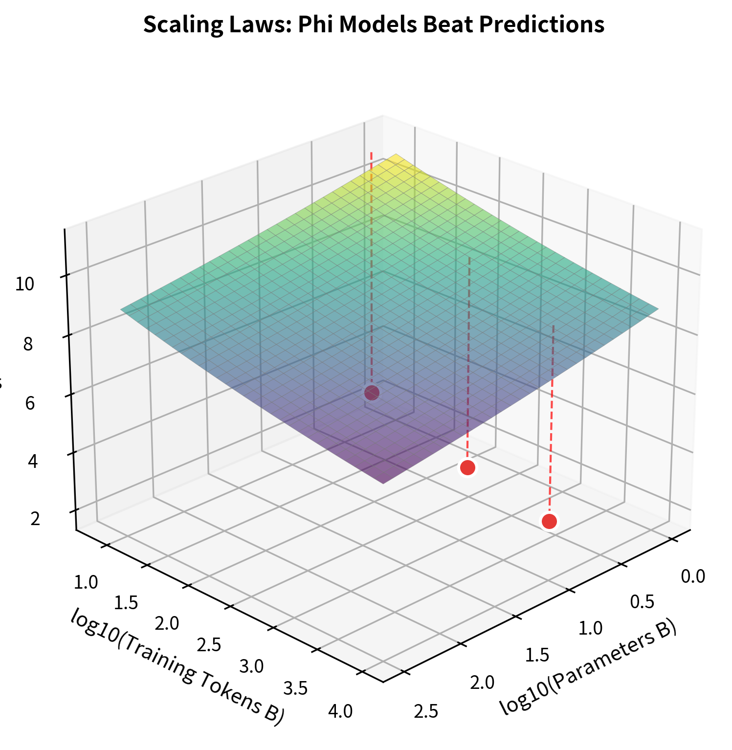
The Phi models consistently achieve lower loss than standard scaling laws predict, demonstrating that data quality can substitute for model size.

But scaling has costs. Training GPT-4 reportedly cost over $100 million. Running inference on 175B parameter models requires specialized hardware. The environmental footprint of training and deploying such models is substantial. If smaller models could achieve similar capabilities, the practical benefits would be enormous.

The Phi project asked a contrarian question: what if the training data, not just the quantity but the quality, is the primary bottleneck? Web-scraped datasets contain enormous amounts of low-quality content: SEO spam, machine-generated text, forum noise, and redundant information. What if we replaced this with carefully crafted educational content?

In[3]:
Code
# Compare model sizes in the Phi family vs contemporaries
phi_models = {
    "Phi-1 (2023)": {"params": 1.3, "training_tokens": 7, "focus": "Code"},
    "Phi-1.5 (2023)": {
        "params": 1.3,
        "training_tokens": 30,
        "focus": "Reasoning",
    },
    "Phi-2 (2023)": {"params": 2.7, "training_tokens": 250, "focus": "General"},
    "Phi-3-mini (2024)": {
        "params": 3.8,
        "training_tokens": 3300,
        "focus": "General",
    },
}

comparison_models = {
    "GPT-3.5": {"params": 175, "training_tokens": 300, "focus": "General"},
    "LLaMA-2-7B": {"params": 7, "training_tokens": 2000, "focus": "General"},
    "Mistral-7B": {"params": 7, "training_tokens": 8000, "focus": "General"},
    "LLaMA-2-70B": {"params": 70, "training_tokens": 2000, "focus": "General"},
}
Out[4]:
Console
Phi Model Family
=================================================================
Model                Params (B)   Tokens (B)     Focus
-----------------------------------------------------------------
Phi-1 (2023)         1.3          7              Code
Phi-1.5 (2023)       1.3          30             Reasoning
Phi-2 (2023)         2.7          250            General
Phi-3-mini (2024)    3.8          3300           General

Comparison Models
-----------------------------------------------------------------
GPT-3.5              175.0        300            General
LLaMA-2-7B           7.0          2000           General
Mistral-7B           7.0          8000           General
LLaMA-2-70B          70.0         2000           General

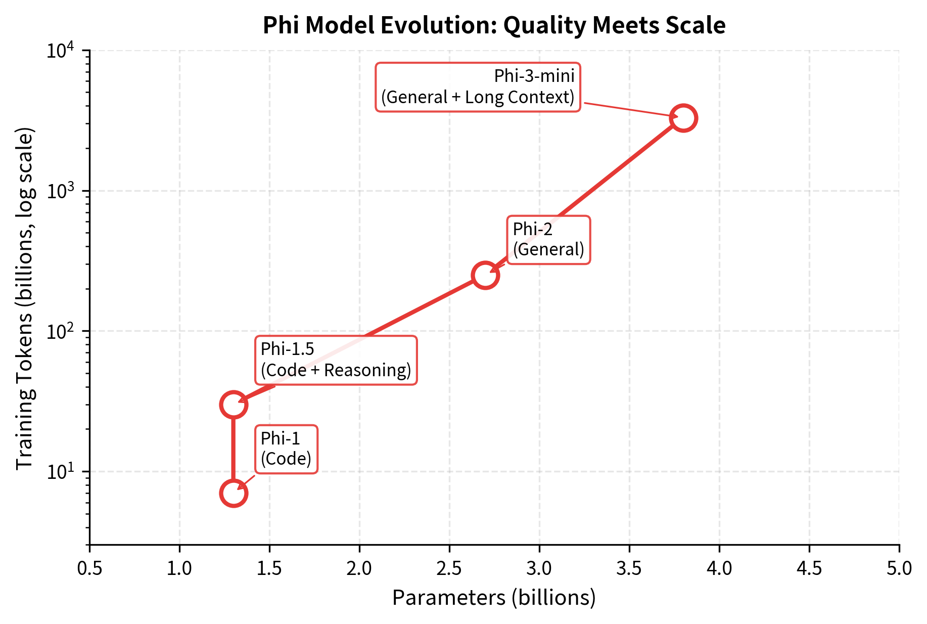
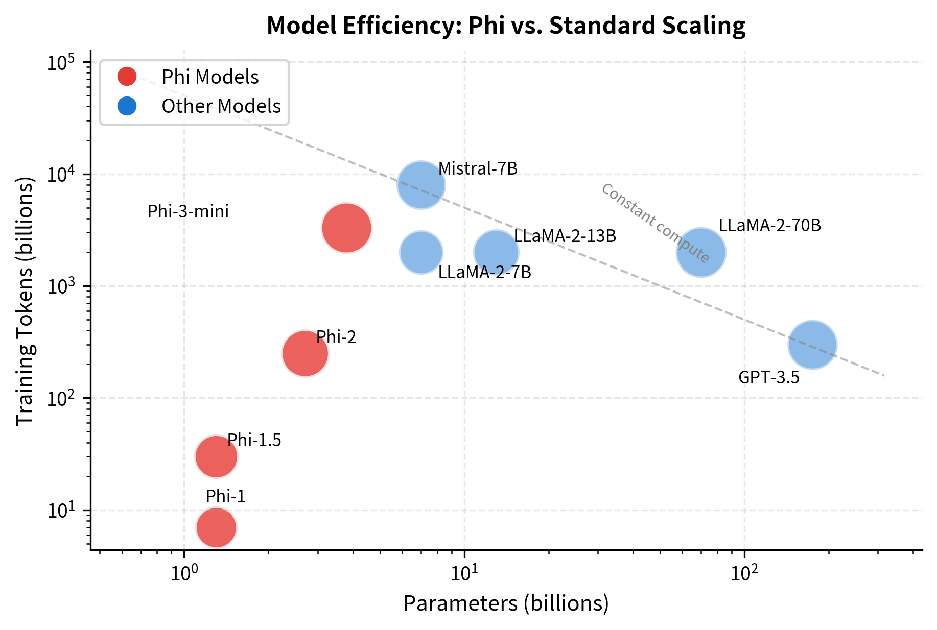
The table reveals the dramatic size difference between Phi models and their competitors. Phi-1 uses only 7B training tokens compared to LLaMA-2's 2,000B, yet achieves competitive performance. This 280x difference in training data volume underscores the impact of data quality.

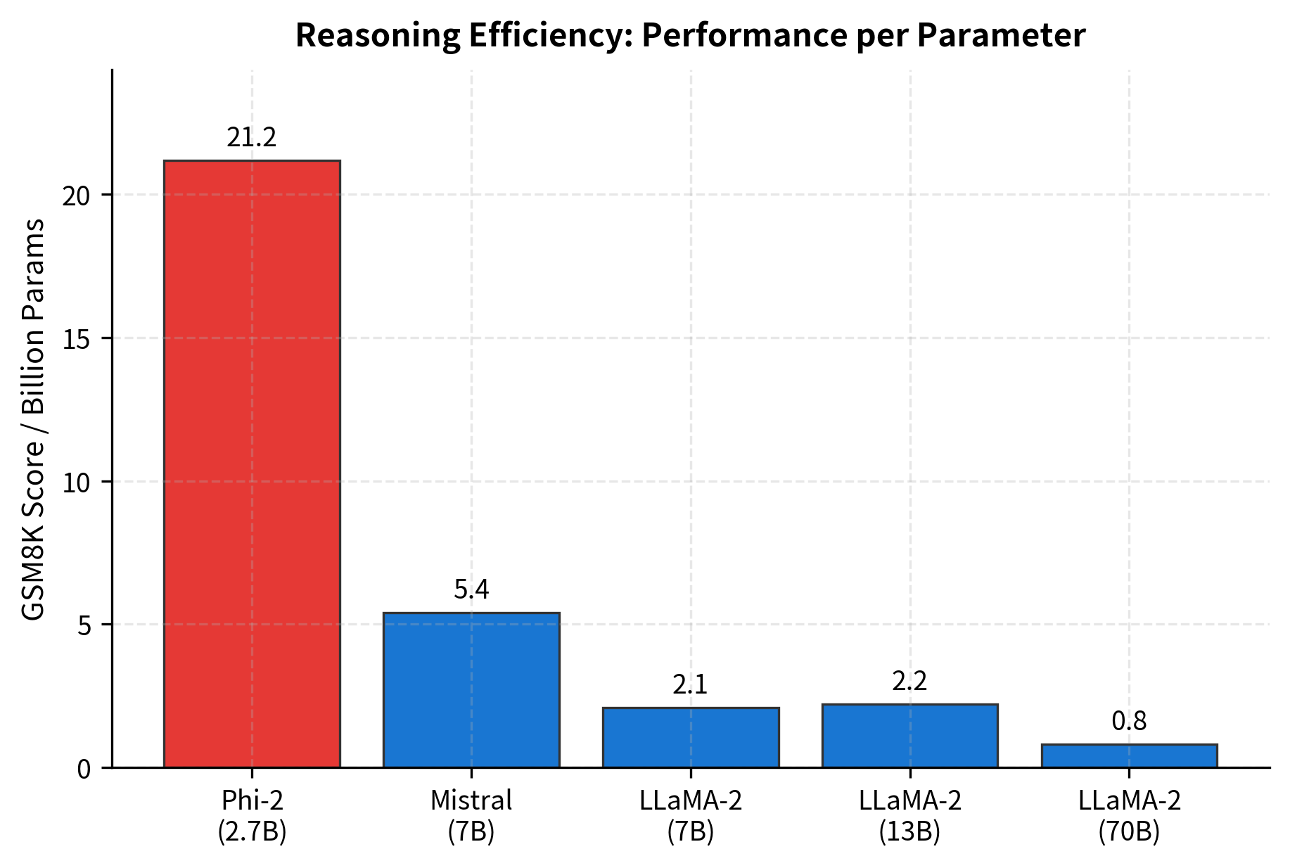
The parameter counts tell a striking story. Phi-1 with 1.3B parameters competed with models 10-100x larger on coding tasks. Phi-2 at 2.7B matched LLaMA-2-7B and approached LLaMA-2-70B on reasoning benchmarks. How is this possible?

Phi-1: Textbooks Are All You Need

The first Phi model focused on code generation. The team hypothesized that the quality of training data for coding tasks could be dramatically improved by generating synthetic "textbook" content rather than relying on scraped code from GitHub.

The Textbook-Quality Data Hypothesis

Real-world code has problems as training data:

  • Noise: Comments may be wrong, outdated, or missing entirely
  • Inconsistency: Different projects use different styles and patterns
  • Complexity: Production code often handles edge cases that obscure core concepts
  • Lack of explanation: Code exists without pedagogical context

A programming textbook, by contrast, introduces concepts systematically, provides clear explanations, uses consistent style, and builds complexity gradually. The Phi team used GPT-3.5 to generate synthetic textbook content covering Python programming concepts.

In[5]:
Code
# Example of the difference between web-scraped vs textbook-style code

# Web-scraped style (from real repositories)
webscrape_example = """
def proc(lst, k=None):
    # TODO: refactor
    res = []
    for i, x in enumerate(lst):
        if k and i >= k:
            break
        if x is not None and str(x).strip():
            res.append(x.lower() if hasattr(x, "lower") else x)
    return res or None  # legacy compat
"""

# Textbook style (synthetic, educational)
textbook_example = '''
def filter_and_normalize(items, limit=None):
    """
    Filter out empty items and normalize strings to lowercase.
    
    This function demonstrates two common list operations:
    1. Filtering: removing None and empty string values
    2. Normalization: converting strings to lowercase
    
    Args:
        items: A list of items to process
        limit: Optional maximum number of items to return
        
    Returns:
        A list of filtered and normalized items
    
    Example:
        >>> filter_and_normalize(["Hello", None, "WORLD", ""])
        ["hello", "world"]
    """
    result = []
    
    for item in items:
        # Skip None values
        if item is None:
            continue
            
        # Skip empty strings (after stripping whitespace)
        if isinstance(item, str) and not item.strip():
            continue
            
        # Normalize strings to lowercase
        if isinstance(item, str):
            result.append(item.lower())
        else:
            result.append(item)
            
        # Stop if we have reached the limit
        if limit is not None and len(result) >= limit:
            break
            
    return result
'''
Out[6]:
Console
Web-Scraped Code vs Textbook-Quality Code
============================================================

--- Web-Scraped Style ---

def proc(lst, k=None):
    # TODO: refactor
    res = []
    for i, x in enumerate(lst):
        if k and i >= k:
            break
        if x is not None and str(x).strip():
            res.append(x.lower() if hasattr(x, "lower") else x)
    return res or None  # legacy compat


--- Textbook Style ---

def filter_and_normalize(items, limit=None):
    """
    Filter out empty items and normalize strings to lowercase.

    This function demonstrates two common list operations:
    1. Filtering: removing None and empty string values
    2. Normalization: converting strings to lowercase

    Args:
        items: A list of items to process
        limit: Optional maximum number of items to return

    Returns:
        A list of filtered and normalized items

    Example:
        >>> filter_and_normalize(["Hello", None, "WORLD", ""])
        ["hello", "world"]
    """
    result = []

    for item in items:
        # Skip None values
        if item is None:
            continue

        # Skip empty strings (after stripping whitespace)
        if isinstance(item, str) and not item.strip():
            continue

        # Normalize strings to lowercase
        if isinstance(item, str):
            result.append(item.lower())
        else:
            result.append(item)

        # Stop if we have reached the limit
        if limit is not None and len(result) >= limit:
            break

    return result

The textbook-style code is longer, but every line serves an educational purpose. Variable names are descriptive. Comments explain the "why," not just the "what." The docstring includes a concrete example. This is the kind of content that teaches programming concepts effectively.

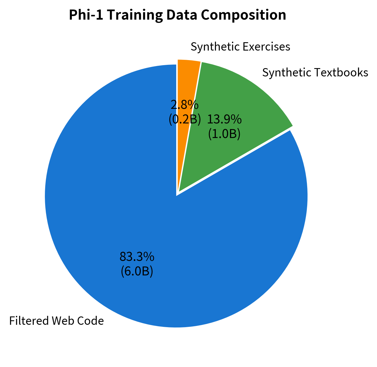
Phi-1 Training Data Composition

Phi-1's training data combined three sources:

  • Filtered Code: About 6B tokens of web code filtered for quality
  • Synthetic Textbooks: 1B tokens of GPT-3.5 generated educational content
  • Synthetic Exercises: Code exercises with solutions, also generated

The filtering process was aggressive. From a large corpus of Python code, only about 20% passed quality filters based on educational value metrics. The synthetic data was generated with careful prompting to produce content resembling high-quality textbooks and courses.

In[7]:
Code
# Phi-1 training data breakdown

phi1_data = {
    "Filtered Web Code": 6.0,
    "Synthetic Textbooks": 1.0,
    "Synthetic Exercises": 0.2,
}

total_tokens = sum(phi1_data.values())
Out[8]:
Visualization
Pie chart showing Phi-1 training data with filtered web code as the largest segment, followed by synthetic textbooks and exercises.
Phi-1 training data composition. Despite using only ~7B tokens total (compared to hundreds of billions for typical models), the high-quality filtered and synthetic data enabled strong code generation performance.

Phi-1 Results

Phi-1's performance surprised the research community. On HumanEval, a benchmark for Python code generation, Phi-1 achieved 50.6% pass@1, comparable to models 10x its size.

In[9]:
Code
# HumanEval benchmark comparison
humaneval_results = {
    "Phi-1 (1.3B)": 50.6,
    "StarCoder (15B)": 33.6,
    "CodeGen-16B": 29.3,
    "GPT-3.5": 48.1,
    "code-davinci-002": 47.0,
}
Out[10]:
Visualization
Bar chart showing Phi-1 matching GPT-3.5 on HumanEval despite having 100x fewer parameters.
HumanEval pass@1 scores comparing Phi-1 to larger code models. Despite being 10-12x smaller than StarCoder and CodeGen, Phi-1 achieves higher accuracy, demonstrating the impact of training data quality.

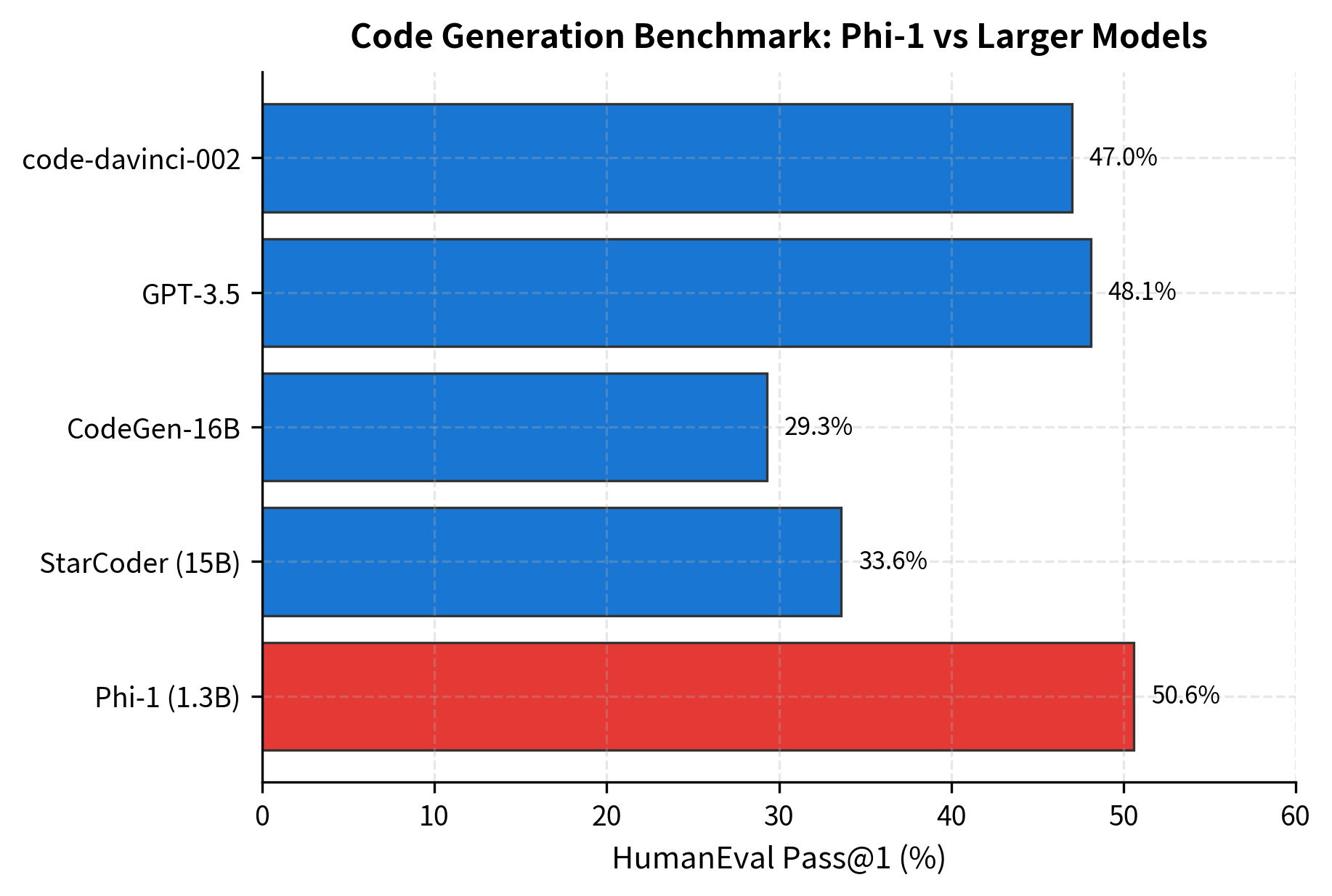
This result validated the core hypothesis: training data quality can substitute for model scale. A small model trained on carefully curated educational content matched or exceeded much larger models trained on raw web data.

Phi-1.5: Extending to Reasoning

Building on Phi-1's success, the team created Phi-1.5 to explore whether the textbook-quality approach generalized beyond coding. Phi-1.5 maintained the 1.3B parameter size but expanded the synthetic data to cover common-sense reasoning and general knowledge.

Synthetic Data for Reasoning

Generating high-quality reasoning data is more challenging than code. Code has clear correctness criteria: it either runs or it doesn't. Reasoning involves nuance, context, and sometimes subjective judgments. The Phi-1.5 team developed prompting strategies to generate textbook-like content for topics including:

  • Science explanations
  • Mathematical reasoning
  • Common-sense scenarios
  • Logical deduction
In[11]:
Code
# Example prompt structure for generating reasoning data
reasoning_prompt_template = """
Write a short educational passage that explains the following concept
in a clear, textbook-like style. Include a concrete example and
explain the reasoning step by step.

Concept: {concept}

The passage should:
1. Introduce the concept clearly
2. Provide a relatable example
3. Walk through the reasoning explicitly
4. Summarize the key insight
"""

example_concepts = [
    "Why ice floats on water",
    "How compound interest works",
    "Why the sky appears blue",
    "The difference between correlation and causation",
]
Out[12]:
Console
Example Concepts for Synthetic Reasoning Data
==================================================
1. Why ice floats on water
2. How compound interest works
3. Why the sky appears blue
4. The difference between correlation and causation

The resulting dataset contained approximately 20B tokens of synthetic textbook content covering diverse reasoning domains, plus 10B tokens of filtered web data selected for educational quality.

Phi-1.5 Architecture

Phi-1.5 used a standard transformer decoder architecture with some notable choices:

  • 24 layers: Relatively deep for a 1.3B model
  • 2048 hidden dimension: Standard width
  • 32 attention heads: With dmodel=2048d_{\text{model}} = 2048 and 32 heads, each head operates on dk=2048/32=64d_k = 2048/32 = 64 dimensions
  • Rotary positional embeddings (RoPE): Same as LLaMA for better length generalization
  • Flash Attention: For efficient training
In[13]:
Code
phi15_config = {
    "Parameters": "1.3B",
    "Layers": 24,
    "Hidden Size": 2048,
    "Attention Heads": 32,
    "Head Dimension": 64,
    "Vocabulary Size": 51200,
    "Context Length": 2048,
    "Positional Encoding": "RoPE",
    "Activation": "GELU",
}
Out[14]:
Console
Phi-1.5 Architecture Configuration
=============================================
Parameters             1.3B
Layers                 24
Hidden Size            2048
Attention Heads        32
Head Dimension         64
Vocabulary Size        51200
Context Length         2048
Positional Encoding    RoPE
Activation             GELU

The configuration shows a relatively deep network (24 layers) for a 1.3B parameter model, with standard choices for hidden size and attention heads. The use of RoPE positional encodings matches LLaMA, enabling better length generalization than absolute positional embeddings.

The architecture itself was not novel. The innovation was entirely in the training data. This strengthens the textbook-quality hypothesis: the same architecture performs dramatically differently depending on what it's trained on.

Phi-2: Scaling Quality

Phi-2 doubled the parameter count to 2.7B and scaled up the synthetic data pipeline. The model demonstrated that the textbook-quality approach continues to provide benefits at larger scales, maintaining competitive performance against models 10-25x its size.

Training Data Strategy

Phi-2's training combined multiple data sources:

  • Synthetic textbooks: Expanded coverage of STEM topics, coding, and reasoning
  • Web data: Heavily filtered for educational content using NLP classifiers
  • Code: High-quality repositories with documentation

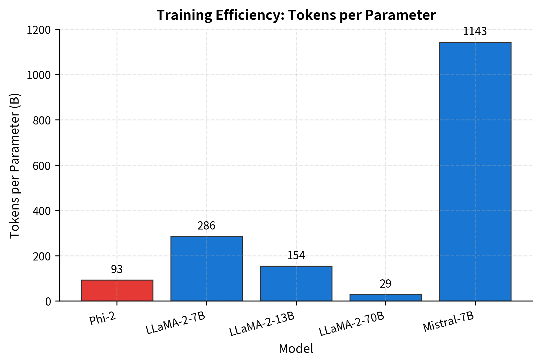
The total training corpus was approximately 250B tokens, still modest compared to LLaMA-2's 2T tokens or GPT-3's 300B tokens, but dramatically higher quality according to Microsoft's metrics.

In[15]:
Code
# Training efficiency comparison
training_efficiency = {
    "Phi-2": {"params": 2.7, "tokens": 250, "tokens_per_param": 92.6},
    "LLaMA-2-7B": {"params": 7, "tokens": 2000, "tokens_per_param": 285.7},
    "LLaMA-2-13B": {"params": 13, "tokens": 2000, "tokens_per_param": 153.8},
    "LLaMA-2-70B": {"params": 70, "tokens": 2000, "tokens_per_param": 28.6},
    "Mistral-7B": {"params": 7, "tokens": 8000, "tokens_per_param": 1142.9},
}
Out[16]:
Visualization
Bar chart comparing tokens-per-parameter ratio across different models.
Training tokens per parameter across models. Phi-2 uses far fewer tokens per parameter than other models, suggesting its performance gains come from data quality rather than quantity. Mistral-7B represents the opposite extreme, training on massive token counts.

Benchmark Performance

Phi-2 achieved remarkable results across diverse benchmarks, often matching or exceeding models with 7-25x more parameters.

In[17]:
Code
# Multi-benchmark comparison
benchmarks = {
    "MMLU": {
        "Phi-2 (2.7B)": 56.3,
        "Mistral-7B": 60.1,
        "LLaMA-2-7B": 45.3,
        "LLaMA-2-13B": 54.8,
        "LLaMA-2-70B": 68.9,
    },
    "GSM8K (Math)": {
        "Phi-2 (2.7B)": 57.2,
        "Mistral-7B": 37.8,
        "LLaMA-2-7B": 14.6,
        "LLaMA-2-13B": 28.7,
        "LLaMA-2-70B": 56.8,
    },
    "HumanEval (Code)": {
        "Phi-2 (2.7B)": 59.0,
        "Mistral-7B": 30.5,
        "LLaMA-2-7B": 12.8,
        "LLaMA-2-13B": 18.3,
        "LLaMA-2-70B": 29.9,
    },
    "MBPP (Code)": {
        "Phi-2 (2.7B)": 60.6,
        "Mistral-7B": 47.5,
        "LLaMA-2-7B": 20.8,
        "LLaMA-2-13B": 30.8,
        "LLaMA-2-70B": 49.8,
    },
}
Out[18]:
Visualization
Grouped bar chart comparing Phi-2 against larger models on MMLU, GSM8K, HumanEval, and MBPP benchmarks.
Phi-2 performance across multiple benchmarks compared to larger models. On GSM8K (mathematical reasoning) and code benchmarks, Phi-2 matches or exceeds LLaMA-2-70B despite being 25x smaller. This demonstrates the particular strength of textbook-quality training for reasoning tasks.

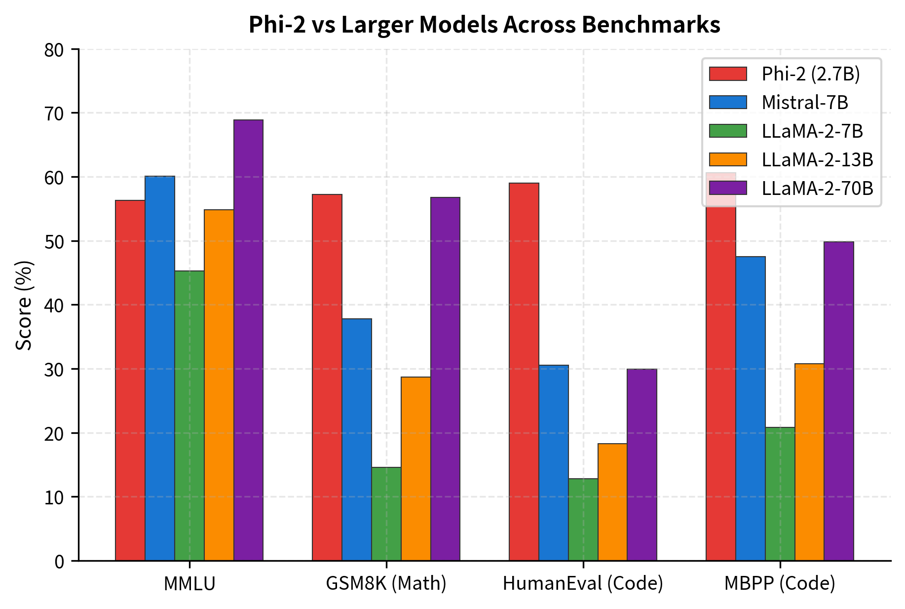
The results reveal an interesting pattern. Phi-2 excels particularly on GSM8K (mathematical reasoning) and code generation, precisely the domains where textbook-quality data provides the clearest advantage. On MMLU (general knowledge), larger models maintain an edge, suggesting that some types of knowledge benefit more from scale than from data quality.

Out[19]:
Visualization
Bar chart showing performance per billion parameters, with Phi-2 dramatically outperforming larger models on efficiency.
Performance per billion parameters on GSM8K (mathematical reasoning). Phi-2 achieves over 21 points per billion parameters, far exceeding the efficiency of larger models. This metric highlights how textbook-quality data enables more effective use of model capacity for reasoning tasks.

Phi-3: Quality Meets Scale

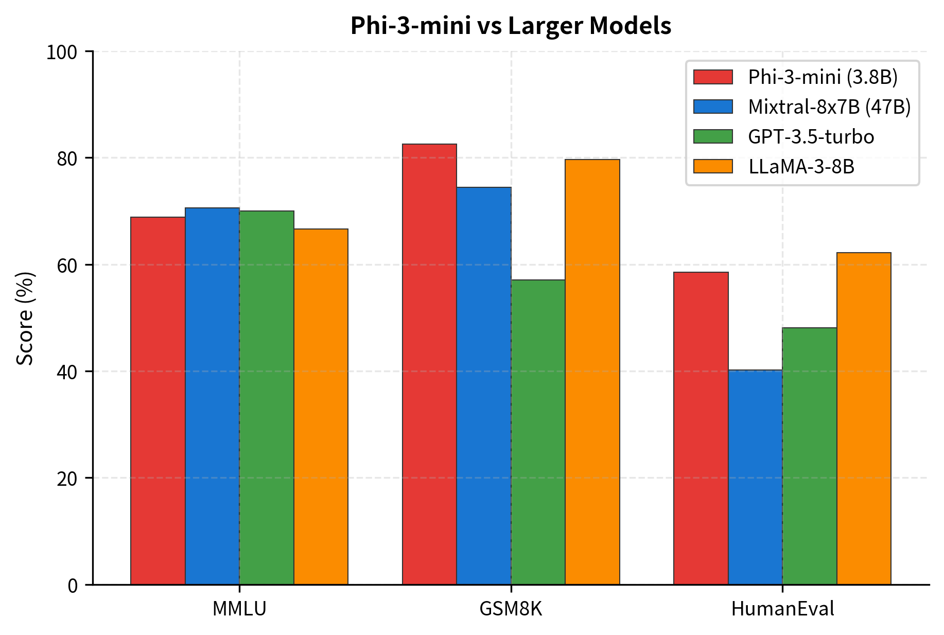
Phi-3, released in 2024, represents the maturation of the textbook-quality approach. With 3.8B parameters in the mini variant, it was trained on an unprecedented 3.3 trillion tokens of heavily filtered and synthetic data. Phi-3 closed the gap with much larger models across nearly all benchmarks.

Data Pipeline Innovations

The Phi-3 training pipeline incorporated several innovations:

  • Multi-stage filtering: Multiple rounds of quality filtering using trained classifiers
  • Diverse synthetic generation: Using multiple large models (not just GPT-4) to generate diverse content
  • Domain coverage expansion: Systematic coverage of academic subjects, professional domains, and world knowledge
  • Instruction tuning: Post-training alignment using synthetic instruction-response pairs
In[20]:
Code
# Phi-3 training stages
phi3_stages = {
    "Stage 1: Web Filtering": {
        "input": "Raw web data",
        "process": "Quality classifiers, deduplication",
        "output": "~1T high-quality tokens",
    },
    "Stage 2: Synthetic Generation": {
        "input": "Topic outlines, skill maps",
        "process": "Multi-model generation, verification",
        "output": "~500B synthetic tokens",
    },
    "Stage 3: Data Mixing": {
        "input": "All filtered and synthetic data",
        "process": "Curriculum-based mixing, repetition tuning",
        "output": "3.3T training tokens",
    },
    "Stage 4: Instruction Tuning": {
        "input": "Pre-trained model",
        "process": "SFT + DPO alignment",
        "output": "Phi-3-instruct variants",
    },
}
Out[21]:
Console
Phi-3 Training Pipeline
=================================================================

Stage 1: Web Filtering
----------------------------------------
  Input: Raw web data
  Process: Quality classifiers, deduplication
  Output: ~1T high-quality tokens

Stage 2: Synthetic Generation
----------------------------------------
  Input: Topic outlines, skill maps
  Process: Multi-model generation, verification
  Output: ~500B synthetic tokens

Stage 3: Data Mixing
----------------------------------------
  Input: All filtered and synthetic data
  Process: Curriculum-based mixing, repetition tuning
  Output: 3.3T training tokens

Stage 4: Instruction Tuning
----------------------------------------
  Input: Pre-trained model
  Process: SFT + DPO alignment
  Output: Phi-3-instruct variants

Phi-3 Model Variants

Phi-3 comes in multiple sizes to suit different deployment scenarios:

In[22]:
Code
phi3_variants = {
    "Phi-3-mini": {
        "params": 3.8,
        "context": 128000,
        "target": "Edge devices, mobile",
    },
    "Phi-3-small": {
        "params": 7,
        "context": 128000,
        "target": "Balanced performance",
    },
    "Phi-3-medium": {
        "params": 14,
        "context": 128000,
        "target": "High performance",
    },
}
Out[23]:
Console
Phi-3 Model Variants
=======================================================
Variant          Parameters   Context      Target Use
-------------------------------------------------------
Phi-3-mini       3.8         B 128,000      Edge devices, mobile
Phi-3-small      7.0         B 128,000      Balanced performance
Phi-3-medium     14.0        B 128,000      High performance
Out[24]:
Visualization
Connected scatter plot showing the progression from Phi-1 to Phi-3-mini in terms of parameters and training tokens.
Evolution of the Phi model family. Each generation increased both model size and training data while maintaining the focus on data quality. The trajectory shows how the textbook-quality approach scaled from a code-focused 1.3B model to a general-purpose 3.8B model competing with much larger systems.

The 128K context length is notable, achieved through RoPE scaling techniques. Standard RoPE is trained for a fixed context length, but the frequencies can be adjusted to extrapolate to longer sequences. Phi-3 uses a technique where the base frequency is modified:

θi=θis=sbase2i/d\theta'_i = \theta_i \cdot s = \frac{s}{\text{base}^{2i/d}}

where ss is a scaling factor that stretches the rotational frequencies, allowing the model to handle longer sequences than it was originally trained on. This allows Phi-3 models to process long documents, complete codebases, or extended conversations while maintaining their small footprint.

Phi-3 Performance

Phi-3-mini matches or exceeds much larger models on key benchmarks:

In[25]:
Code
phi3_comparison = {
    "MMLU": {
        "Phi-3-mini (3.8B)": 68.8,
        "Mixtral-8x7B (47B)": 70.6,
        "GPT-3.5-turbo": 70.0,
        "LLaMA-3-8B": 66.6,
    },
    "GSM8K": {
        "Phi-3-mini (3.8B)": 82.5,
        "Mixtral-8x7B (47B)": 74.4,
        "GPT-3.5-turbo": 57.1,
        "LLaMA-3-8B": 79.6,
    },
    "HumanEval": {
        "Phi-3-mini (3.8B)": 58.5,
        "Mixtral-8x7B (47B)": 40.2,
        "GPT-3.5-turbo": 48.1,
        "LLaMA-3-8B": 62.2,
    },
}
Out[26]:
Visualization
Grouped bar chart showing Phi-3-mini matching much larger models on MMLU, GSM8K, and HumanEval.
Phi-3-mini performance compared to larger models. Despite having only 3.8B parameters, Phi-3-mini matches GPT-3.5 on MMLU and significantly outperforms it on mathematical reasoning (GSM8K). This represents a major efficiency breakthrough.

Code Implementation: Phi-Style Attention

To truly understand how Phi models work, we need to examine their core computational mechanism: multi-head attention with rotary positional embeddings (RoPE). While the architecture is standard, implementing it from scratch reveals the elegant mathematics that enables transformers to process sequences.

Our implementation journey proceeds through three stages:

  1. Positional encoding: How RoPE embeds position information through rotation
  2. Attention computation: How queries, keys, and values interact to produce contextual representations
  3. Integration: How these components combine in a complete attention layer

Understanding Rotary Position Embeddings

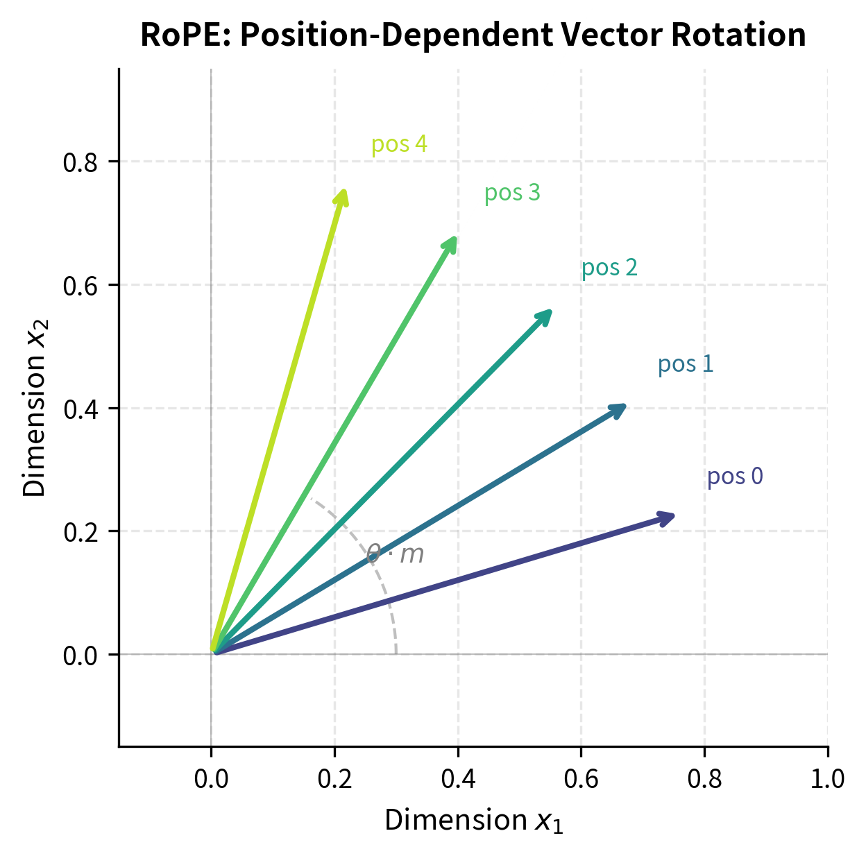
Before diving into code, let's build intuition for why positional encoding matters. A transformer's attention mechanism computes similarity between all pairs of tokens, but this computation is inherently position-agnostic. The same query-key pair produces the same similarity score regardless of where the tokens appear in the sequence. Yet position clearly matters: "The cat sat on the mat" has different meaning than "mat the on sat cat The."

Traditional approaches add positional embeddings to token embeddings before attention. RoPE takes a different approach: it encodes position by rotating the query and key vectors in embedding space. The key insight is that rotation preserves vector magnitudes while changing the angle between vectors. When we compute the dot product (attention score) between a rotated query and key, the result depends on their relative positions, not just their content.

Think of it geometrically: if we rotate a query vector by angle θq\theta_q and a key vector by angle θk\theta_k, their dot product depends on the difference θqθk\theta_q - \theta_k. By making these rotation angles position-dependent, we encode relative position directly into the attention computation.

In[27]:
Code
import numpy as np


def apply_rotary_embeddings(x, cos, sin):
    """
    Apply rotary positional embeddings to input tensor.

    RoPE rotates pairs of dimensions in the embedding space by
    position-dependent angles, enabling the model to encode
    relative positions through the attention dot product.

    Args:
        x: Input tensor of shape (batch, heads, seq_len, head_dim)
        cos: Cosine of rotation angles (seq_len, head_dim)
        sin: Sine of rotation angles (seq_len, head_dim)

    Returns:
        Rotated tensor of same shape as input
    """
    # Split into pairs for rotation
    x1 = x[..., ::2]  # Even indices
    x2 = x[..., 1::2]  # Odd indices

    # Reshape cos/sin for broadcasting
    cos = cos[np.newaxis, np.newaxis, :, :]
    sin = sin[np.newaxis, np.newaxis, :, :]

    # Apply rotation
    rotated_x1 = x1 * cos - x2 * sin
    rotated_x2 = x1 * sin + x2 * cos

    # Interleave back together
    result = np.empty_like(x)
    result[..., ::2] = rotated_x1
    result[..., 1::2] = rotated_x2

    return result


def compute_rope_frequencies(head_dim, max_seq_len, base=10000):
    """
    Compute RoPE frequency components.

    These frequencies determine how quickly each dimension
    rotates as position increases, with lower-index dimensions
    rotating more slowly to capture longer-range patterns.
    """
    # Frequency for each dimension pair
    dim_indices = np.arange(0, head_dim, 2)
    freqs = 1.0 / (base ** (dim_indices / head_dim))

    # Position indices
    positions = np.arange(max_seq_len)

    # Compute angles: (seq_len, head_dim/2)
    angles = np.outer(positions, freqs)

    # Expand to full head_dim by repeating
    cos = np.cos(angles)
    sin = np.sin(angles)

    return cos, sin

The Mathematics of Rotation

RoPE applies a 2D rotation to each pair of consecutive dimensions in the embedding. A 2D rotation by angle θ\theta transforms a vector (x1,x2)(x_1, x_2) to:

(x1x2)=(cosθsinθsinθcosθ)(x1x2)\begin{pmatrix} x'_1 \\ x'_2 \end{pmatrix} = \begin{pmatrix} \cos\theta & -\sin\theta \\ \sin\theta & \cos\theta \end{pmatrix} \begin{pmatrix} x_1 \\ x_2 \end{pmatrix}

This is exactly what our apply_rotary_embeddings function computes: for each pair of dimensions, it applies the rotation using the precomputed cosine and sine values.
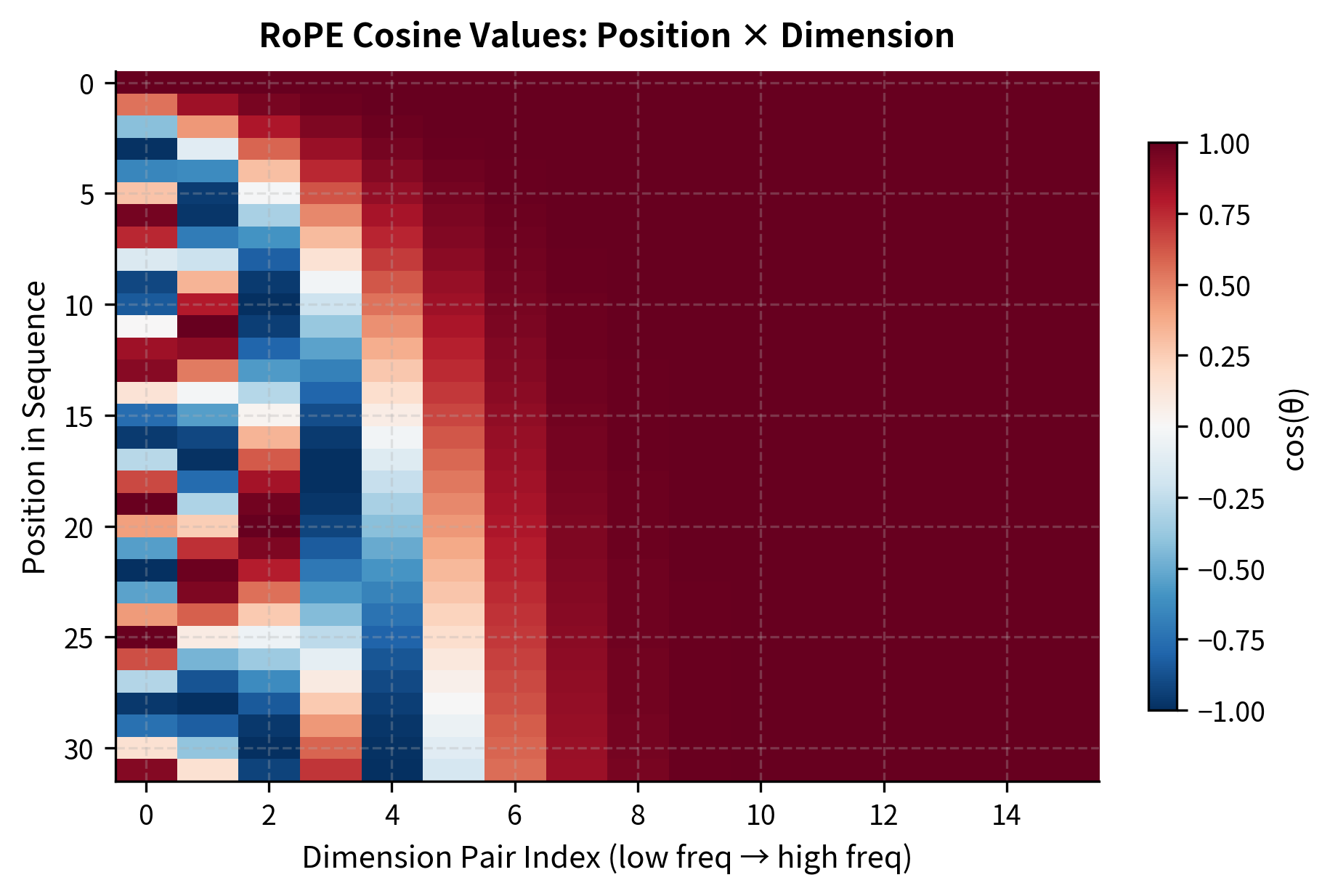
Out[28]:
Visualization
2D plot showing a vector being rotated to different angles based on sequence position, illustrating the RoPE mechanism.
Geometric visualization of RoPE. The same embedding vector is rotated by different angles depending on its position in the sequence. Position 0 remains unrotated (0°), while later positions rotate progressively. When computing attention, the dot product between rotated queries and keys naturally encodes relative position.

The rotation angle for position mm and dimension pair ii is computed as:

θm,i=mθi=m1base2i/d\theta_{m,i} = m \cdot \theta_i = m \cdot \frac{1}{\text{base}^{2i/d}}

where:

  • mm: the position index in the sequence (0, 1, 2, ...)
  • ii: the dimension pair index (0, 1, 2, ..., d/21d/2 - 1)
  • dd: the head dimension (e.g., 64)
  • base\text{base}: a hyperparameter controlling the frequency scale (typically 10,000)

Lower-indexed dimensions rotate more slowly (smaller θi\theta_i), capturing longer-range positional relationships, while higher-indexed dimensions rotate faster, encoding fine-grained local position information.

This frequency hierarchy is crucial: it allows the model to represent both local patterns (through high-frequency dimensions) and long-range dependencies (through low-frequency dimensions) simultaneously. Let's see this in practice:

Out[29]:
Console
RoPE Frequency Computation
==================================================
Head dimension: 64
Sequence length: 8
Cosine shape: (8, 32)
Sine shape: (8, 32)

First 4 positions, first 4 frequency components:

Cosine values:
[[ 1.     1.     1.     1.   ]
 [ 0.54   0.732  0.846  0.912]
 [-0.416  0.071  0.431  0.665]
 [-0.99  -0.628 -0.116  0.301]]

Sine values:
[[0.    0.    0.    0.   ]
 [0.841 0.682 0.533 0.409]
 [0.909 0.997 0.902 0.747]
 [0.141 0.778 0.993 0.954]]

The output shows how RoPE frequencies vary across positions and dimensions. Notice that the first column (lowest frequency) changes slowly across positions, while higher-frequency components (rightmost columns) oscillate more rapidly. At position 0, all sine values are 0 and cosine values are 1, meaning no rotation occurs. As position increases, the rotation angles grow, with higher-indexed dimensions accumulating rotation faster.

Out[30]:
Visualization
Heatmap showing RoPE cosine values across 32 positions and 16 dimension pairs, with slower oscillation on the left and faster on the right.
RoPE frequency patterns across dimensions and positions. Lower-indexed dimensions (left columns) change slowly across positions, capturing long-range dependencies. Higher-indexed dimensions oscillate rapidly, encoding fine-grained local position information. This frequency hierarchy enables transformers to model relationships at multiple scales simultaneously.

From Position Encoding to Attention

With position encoding understood, we can now build the complete attention mechanism. The core idea of attention is simple: each position in the sequence should be able to gather information from other positions, weighted by relevance. A query asks "what information do I need?", keys answer "here's what I have", and values provide the actual information to aggregate.

The mathematical formulation captures this intuition precisely. The core attention computation follows the standard scaled dot-product formula:

Attention(Q,K,V)=softmax(QKTdk)V\text{Attention}(Q, K, V) = \text{softmax}\left(\frac{QK^T}{\sqrt{d_k}}\right)V

where:

  • QRn×dkQ \in \mathbb{R}^{n \times d_k}: the query matrix, where each row represents a position asking "what should I attend to?"
  • KRn×dkK \in \mathbb{R}^{n \times d_k}: the key matrix, where each row represents a position answering "here's what I contain"
  • VRn×dvV \in \mathbb{R}^{n \times d_v}: the value matrix, containing the actual information to be aggregated
  • dkd_k: the key/query dimension (typically 64 in Phi models)
  • nn: the sequence length
  • dk\sqrt{d_k}: scaling factor that prevents dot products from becoming too large

The softmax normalizes attention scores so each query position's weights sum to 1, creating a valid probability distribution over key positions.

Why divide by dk\sqrt{d_k}? As the dimension dkd_k grows, dot products tend to grow in magnitude (they're sums of dkd_k terms). Large dot products push softmax into regions where gradients vanish, making training unstable. The scaling factor keeps the variance of dot products roughly constant regardless of dkd_k.

Putting It All Together: The PhiAttention Class

Now we can combine RoPE with scaled dot-product attention in a complete implementation. The PhiAttention class orchestrates the full computation:

  1. Project input to queries, keys, and values using learned weight matrices
  2. Reshape to separate attention heads (each head attends independently)
  3. Apply RoPE to queries and keys (encoding position)
  4. Compute scaled dot-product attention
  5. Apply causal mask for autoregressive generation
  6. Project output back to model dimension
In[31]:
Code
class PhiAttention:
    """
    Multi-head attention as used in Phi models.

    Combines standard scaled dot-product attention with:
    - Rotary positional embeddings (RoPE)
    - Pre-normalization
    - Flash Attention compatibility (not implemented here)
    """

    def __init__(self, hidden_size=2048, num_heads=32, head_dim=64, seed=42):
        """
        Initialize attention weights.

        Args:
            hidden_size: Model hidden dimension
            num_heads: Number of attention heads
            head_dim: Dimension per attention head
            seed: Random seed for initialization
        """
        self.hidden_size = hidden_size
        self.num_heads = num_heads
        self.head_dim = head_dim

        np.random.seed(seed)

        # Phi uses small initialization scale
        scale = 0.02

        # Query, Key, Value projections
        self.W_q = np.random.randn(hidden_size, num_heads * head_dim) * scale
        self.W_k = np.random.randn(hidden_size, num_heads * head_dim) * scale
        self.W_v = np.random.randn(hidden_size, num_heads * head_dim) * scale

        # Output projection
        self.W_o = np.random.randn(num_heads * head_dim, hidden_size) * scale

        # Pre-compute RoPE frequencies for max sequence length
        self.max_seq_len = 2048
        self.cos, self.sin = compute_rope_frequencies(
            head_dim // 2 * 2,  # Ensure even
            self.max_seq_len,
        )

    def forward(self, x, mask=None):
        """
        Compute attention output.

        Args:
            x: Input tensor (batch, seq_len, hidden_size)
            mask: Optional causal mask (seq_len, seq_len)

        Returns:
            output: Attention output (batch, seq_len, hidden_size)
            weights: Attention weights (batch, heads, seq_len, seq_len)
        """
        batch, seq_len, _ = x.shape

        # Project to Q, K, V
        Q = x @ self.W_q  # (batch, seq_len, num_heads * head_dim)
        K = x @ self.W_k
        V = x @ self.W_v

        # Reshape to (batch, num_heads, seq_len, head_dim)
        Q = Q.reshape(batch, seq_len, self.num_heads, self.head_dim)
        Q = Q.transpose(0, 2, 1, 3)
        K = K.reshape(batch, seq_len, self.num_heads, self.head_dim)
        K = K.transpose(0, 2, 1, 3)
        V = V.reshape(batch, seq_len, self.num_heads, self.head_dim)
        V = V.transpose(0, 2, 1, 3)

        # Apply RoPE to Q and K
        cos_slice = self.cos[:seq_len]
        sin_slice = self.sin[:seq_len]
        Q = apply_rotary_embeddings(Q, cos_slice, sin_slice)
        K = apply_rotary_embeddings(K, cos_slice, sin_slice)

        # Compute attention scores using scaled dot-product attention
        # The scaling factor sqrt(d_k) prevents dot products from growing
        # too large as the head dimension increases
        scale = np.sqrt(self.head_dim)
        scores = (Q @ K.transpose(0, 1, 3, 2)) / scale

        # Apply causal mask if provided (set masked positions to -inf)
        if mask is not None:
            scores = np.where(mask, scores, -1e9)

        # Softmax converts scores to attention weights that sum to 1
        exp_scores = np.exp(scores - scores.max(axis=-1, keepdims=True))
        weights = exp_scores / exp_scores.sum(axis=-1, keepdims=True)

        # Weighted sum of values produces the attention output
        output = weights @ V  # (batch, heads, seq_len, head_dim)

        # Reshape back
        output = output.transpose(
            0, 2, 1, 3
        )  # (batch, seq_len, heads, head_dim)
        output = output.reshape(batch, seq_len, self.num_heads * self.head_dim)

        # Output projection
        output = output @ self.W_o

        return output, weights

The implementation follows the mathematical formulation closely. Notice how the forward method mirrors our six-step process: projection, reshaping, RoPE application, attention computation, masking, and output projection.

Key implementation details worth noting:

  • Small initialization scale (0.02): Phi uses smaller weight initialization than some models, which can help training stability
  • Pre-computed RoPE frequencies: We compute cosine and sine values once and slice them per sequence length, avoiding redundant computation
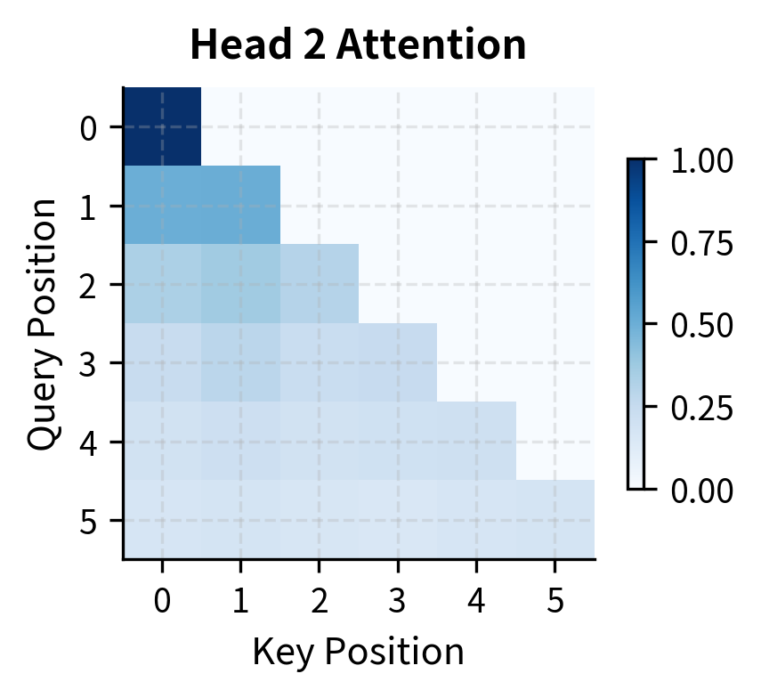
  • Causal masking: The mask ensures position ii can only attend to positions i\leq i, enabling autoregressive generation

Testing the Implementation

Let's verify our attention layer works correctly by processing a small sequence and examining the outputs:

In[32]:
Code
# Test the attention implementation
batch_size = 1
seq_len = 6
hidden_size = 256
num_heads = 4
head_dim = 64

# Create test input
np.random.seed(123)
x = np.random.randn(batch_size, seq_len, hidden_size)

# Create causal mask
causal_mask = np.tril(np.ones((seq_len, seq_len), dtype=bool))

# Initialize and run attention
attention = PhiAttention(
    hidden_size=hidden_size, num_heads=num_heads, head_dim=head_dim
)

output, weights = attention.forward(x, mask=causal_mask)
Out[33]:
Console
Phi-Style Attention Test
==================================================
Input shape:  (1, 6, 256)
Output shape: (1, 6, 256)
Weights shape: (1, 4, 6, 6)

Attention weights sum per query (should be 1.0):
[1. 1. 1. 1. 1. 1.]

The output confirms our implementation is working correctly. The input and output shapes match (preserving dimensions through the attention layer), and each row of attention weights sums to exactly 1.0, indicating proper softmax normalization. The weights tensor has shape (1, 4, 6, 6), representing 4 attention heads each producing a 6x6 attention matrix for the 6-position sequence.

Visualizing Attention Patterns

The causal mask creates a distinctive lower-triangular pattern in the attention weights. This pattern is fundamental to autoregressive language modeling: when predicting position 5, the model can only see positions 0-5, not future positions 6 and beyond. Let's visualize this:

Out[34]:
Visualization
Heatmap of attention weights for head 1 showing causal lower-triangular pattern with strong diagonal emphasis.
Attention pattern from head 1 showing strong diagonal focus. Each position primarily attends to itself and immediate neighbors.
Heatmap of attention weights for head 2 showing a different attention distribution pattern.
Head 2 shows a different pattern, distributing attention more broadly across earlier positions. This diversity allows the model to capture both local and global context.

Understanding Phi's Efficiency

Why can Phi models achieve competitive performance with fewer parameters? Several factors contribute:

Data Efficiency

The textbook-quality approach maximizes learning per token. Instead of exposing the model to repetitive or low-quality content, every training example teaches something. This is analogous to the difference between learning from a well-designed curriculum versus random exposure to information.

Out[35]:
Visualization
Bubble chart showing Phi models achieving competitive performance with fewer parameters and training tokens compared to LLaMA and GPT models.
Parameter efficiency comparison across language models. The x-axis shows model parameters (log scale), the y-axis shows training tokens (log scale), and bubble size indicates approximate benchmark performance. Phi models cluster in the lower-left, achieving strong performance with fewer resources. The dashed line represents constant compute (parameters × tokens).

High-quality data allows Phi models to achieve comparable performance to much larger models while using significantly fewer training tokens. The key insight is that learning per token can vary by an order of magnitude depending on data quality.

Capacity Utilization

Large models trained on noisy data may dedicate significant capacity to memorizing spurious patterns, formatting quirks, or redundant information. A smaller model trained on cleaner data can allocate more of its limited capacity to genuinely useful patterns.

Reasoning Focus

Phi's training data emphasizes step-by-step reasoning, code with explanations, and mathematical derivations. This may help the model develop stronger reasoning circuits compared to models that see mostly surface-level text patterns.

Limitations and Considerations

Despite their impressive efficiency, Phi models have limitations worth understanding.

Knowledge breadth: While Phi excels at reasoning and code, models trained on more diverse web data may have broader world knowledge. A larger model might know more obscure facts simply because it has seen more text. Phi's focus on high-quality synthetic data means it may miss niche domains that weren't explicitly covered in the curriculum.

Long-tail capabilities: The textbook-quality approach works well for structured domains like programming and mathematics where educational content is well-defined. For more open-ended creative tasks or understanding of cultural nuance, the synthetic data generation process may not capture the full richness needed.

Synthetic data limitations: While synthetic data can be high-quality, it ultimately reflects the capabilities and biases of the models that generated it. If the teacher models (like GPT-3.5 or GPT-4) have systematic blind spots, these may propagate to Phi. There's also a risk of "mode collapse" where synthetic data becomes repetitive or stylistically narrow.

Benchmark saturation: As Phi models achieve strong benchmark performance, questions arise about whether benchmarks truly measure the capabilities we care about. A model optimized for textbook-style reasoning might excel at clean benchmark problems while struggling with messy real-world inputs.

In[36]:
Code
# Areas where larger models may still have advantages
tradeoffs = {
    "Phi Advantages": [
        "Mathematical reasoning",
        "Code generation",
        "Step-by-step explanations",
        "Inference efficiency",
        "Edge deployment",
    ],
    "Large Model Advantages": [
        "Broad world knowledge",
        "Rare/niche topics",
        "Creative writing",
        "Cultural nuance",
        "Few-shot learning on new tasks",
    ],
}
Out[37]:
Console
Phi vs Large Models: Tradeoffs
=======================================================

Phi Advantages:
  • Mathematical reasoning
  • Code generation
  • Step-by-step explanations
  • Inference efficiency
  • Edge deployment

Large Model Advantages:
  • Broad world knowledge
  • Rare/niche topics
  • Creative writing
  • Cultural nuance
  • Few-shot learning on new tasks

Deployment and Practical Use

Phi models are designed for efficient deployment. Their small size enables scenarios that would be impractical with larger models.

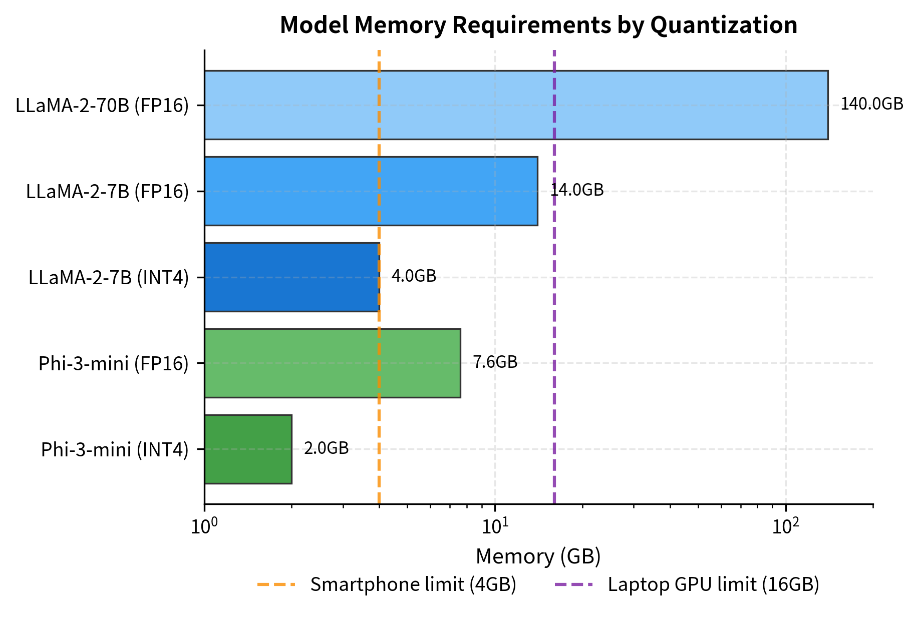
Edge deployment: Phi-3-mini can run on smartphones and laptops without cloud connectivity. This enables privacy-preserving applications where user data never leaves the device.

Quantization: The small parameter count makes quantization more effective. Quantization reduces memory by representing weights with fewer bits. For a model with NN parameters, the memory requirement scales as:

Memory=N×b8 bytes\text{Memory} = N \times \frac{b}{8} \text{ bytes}

where:

  • NN: the number of model parameters
  • bb: the number of bits per parameter (e.g., 16 for FP16, 4 for INT4)

A 4-bit quantized Phi-3-mini (3.8B parameters) requires approximately 3.8×109×0.52GB3.8 \times 10^9 \times 0.5 \approx 2\text{GB} of memory while maintaining most of its capabilities.

Batched inference: The smaller memory footprint allows processing more requests simultaneously on a single GPU, reducing per-query costs.

Fine-tuning: With fewer parameters, fine-tuning Phi models requires less compute and memory, making customization accessible to more users.

In[38]:
Code
# Deployment scenarios
deployment_specs = {
    "Phi-3-mini (FP16)": {
        "memory_gb": 7.6,
        "smartphone": False,
        "laptop_gpu": True,
        "server_gpu": True,
    },
    "Phi-3-mini (INT4)": {
        "memory_gb": 2.0,
        "smartphone": True,
        "laptop_gpu": True,
        "server_gpu": True,
    },
    "LLaMA-2-7B (FP16)": {
        "memory_gb": 14,
        "smartphone": False,
        "laptop_gpu": False,
        "server_gpu": True,
    },
    "LLaMA-2-70B (FP16)": {
        "memory_gb": 140,
        "smartphone": False,
        "laptop_gpu": False,
        "server_gpu": True,
    },
}
Out[39]:
Console
Deployment Feasibility by Platform
=================================================================
Model                     Memory     Phone    Laptop   Server
-----------------------------------------------------------------
Phi-3-mini (FP16)         7.6       GB ✗        ✓        ✓
Phi-3-mini (INT4)         2.0       GB ✓        ✓        ✓
LLaMA-2-7B (FP16)         14.0      GB ✗        ✗        ✓
LLaMA-2-70B (FP16)        140.0     GB ✗        ✗        ✓
Out[40]:
Visualization
Horizontal bar chart showing memory requirements for different models and quantization levels, with device memory thresholds marked.
Memory requirements across models and quantization levels. INT4 quantization reduces Phi-3-mini to just 2GB, enabling smartphone deployment. The horizontal dashed lines show typical device memory limits, illustrating why Phi models can run on devices where LLaMA cannot.

Summary

The Phi model family demonstrates that data quality can substitute for model scale. By training on carefully curated "textbook-quality" data, Phi models achieve remarkable efficiency.

The key innovations and insights from this chapter:

  • Textbook-quality hypothesis: Carefully curated educational content enables more efficient learning than raw web data. Quality trumps quantity when data is engineered for pedagogical value.

  • Synthetic data generation: Using larger models to generate structured, educational training data creates a new paradigm for dataset construction. The resulting data can teach concepts more effectively than naturally-occurring text.

  • Evolution across versions: Phi-1 proved the concept for code, Phi-1.5 extended it to reasoning, Phi-2 scaled the approach, and Phi-3 achieved near-parity with models 10-25x larger.

  • Architecture simplicity: Phi uses standard transformer architecture with RoPE and Flash Attention. The innovation is entirely in the training data, validating that architecture alone doesn't determine capability.

  • Deployment efficiency: Small parameter counts enable edge deployment, efficient quantization, and lower inference costs. Phi-3-mini can run on devices where larger models are impractical.

  • Tradeoffs: Phi models excel at structured reasoning tasks but may have narrower knowledge coverage than larger models trained on diverse web data. The synthetic data approach has inherent limitations around diversity and coverage.

The Phi series challenges us to think differently about model development. Rather than assuming that scale is the only path to capability, the textbook-quality approach suggests that thoughtful data curation may be equally important. As the field matures, we may see convergence between these strategies: large-scale training on carefully filtered and augmented data that combines the benefits of both approaches.

Key Parameters

When working with or fine-tuning Phi models, the following parameters have the most significant impact:

Model Selection

  • Model variant: Choose Phi-3-mini (3.8B) for edge deployment and mobile, Phi-3-small (7B) for balanced performance, or Phi-3-medium (14B) for maximum capability. The mini variant offers the best efficiency-to-capability ratio for most use cases.

Inference Configuration

  • Context length: Phi-3 supports up to 128K tokens through RoPE scaling. Use shorter contexts (4K-8K) for faster inference; extend to 128K only when processing long documents.
  • Quantization: INT4 quantization reduces memory by approximately 4x with minimal quality degradation. Recommended for edge deployment; use FP16 or BF16 for maximum quality on server hardware.
  • Batch size: Smaller model size allows larger batch sizes on the same hardware, improving throughput for high-volume applications.

Fine-tuning Configuration

  • LoRA rank: Ranks of 16-64 work well for domain adaptation. Lower ranks (8-16) suffice for style transfer; higher ranks (32-64) for learning new capabilities.
  • Learning rate: Use 1e-5 to 5e-5 for full fine-tuning, 1e-4 to 3e-4 for LoRA. Phi's smaller size makes it more sensitive to learning rate than larger models.
  • Training epochs: 1-3 epochs typically sufficient given the model's strong base capabilities. Monitor for overfitting on small datasets.

The next chapter examines other efficient model architectures and techniques for reducing the computational requirements of large language models while maintaining their capabilities.

Quiz

Ready to test your understanding? Take this quick quiz to reinforce what you've learned about Phi models and the textbook-quality data hypothesis.

Loading component...
Track your reading progress

Sign in to mark chapters as read and track your learning journey

Sign in →

Comments

Reference

BIBTEXAcademic
@misc{phimodelshowdataqualitybeatsmodelscale, author = {Michael Brenndoerfer}, title = {Phi Models: How Data Quality Beats Model Scale}, year = {2025}, url = {https://mbrenndoerfer.com/writing/phi-models-textbook-quality-data}, organization = {mbrenndoerfer.com}, note = {Accessed: 2025-12-19} }
APAAcademic
Michael Brenndoerfer (2025). Phi Models: How Data Quality Beats Model Scale. Retrieved from https://mbrenndoerfer.com/writing/phi-models-textbook-quality-data
MLAAcademic
Michael Brenndoerfer. "Phi Models: How Data Quality Beats Model Scale." 2025. Web. 12/19/2025. <https://mbrenndoerfer.com/writing/phi-models-textbook-quality-data>.
CHICAGOAcademic
Michael Brenndoerfer. "Phi Models: How Data Quality Beats Model Scale." Accessed 12/19/2025. https://mbrenndoerfer.com/writing/phi-models-textbook-quality-data.
HARVARDAcademic
Michael Brenndoerfer (2025) 'Phi Models: How Data Quality Beats Model Scale'. Available at: https://mbrenndoerfer.com/writing/phi-models-textbook-quality-data (Accessed: 12/19/2025).
SimpleBasic
Michael Brenndoerfer (2025). Phi Models: How Data Quality Beats Model Scale. https://mbrenndoerfer.com/writing/phi-models-textbook-quality-data
Michael Brenndoerfer

About the author: Michael Brenndoerfer

All opinions expressed here are my own and do not reflect the views of my employer.

Michael currently works as an Associate Director of Data Science at EQT Partners in Singapore, leading AI and data initiatives across private capital investments.

With over a decade of experience spanning private equity, management consulting, and software engineering, he specializes in building and scaling analytics capabilities from the ground up. He has published research in leading AI conferences and holds expertise in machine learning, natural language processing, and value creation through data.

Stay updated

Get notified when I publish new articles on data and AI, private equity, technology, and more.

No spam, unsubscribe anytime.

or

Create a free account to unlock exclusive features, track your progress, and join the conversation.

No popupsUnobstructed readingCommenting100% Free