

Learn how weight tying reduces transformer parameters by sharing the input embedding and output projection matrices. Covers the theoretical justification, implementation details, encoder-decoder tying, and when to use this technique.

This article is part of the free-to-read Language AI Handbook
Choose your expertise level to adjust how many terms are explained. Beginners see more tooltips, experts see fewer to maintain reading flow. Hover over underlined terms for instant definitions.
Weight Tying
Language models contain two large embedding matrices that seem to serve different purposes: one converts input tokens into vectors, and another converts output vectors back into token probabilities. But these matrices are surprisingly similar in structure, both mapping between the same vocabulary and the same hidden dimension. Weight tying exploits this similarity by making them literally the same matrix, cutting parameter count and often improving model quality.
In this chapter, you'll learn how weight tying works, why it makes theoretical sense, and when to use it in your own models. We'll implement tied embeddings from scratch and examine the practical considerations that determine whether tying helps or hurts.
The Two Embedding Matrices
Before diving into weight tying, let's be clear about what we're tying together. A language model has two distinct embedding operations that bookend the transformer layers.
The input embedding matrix converts discrete token indices into continuous vectors. Each row contains the learned embedding for one vocabulary token:
where:
- : the input embedding matrix of shape
- : the input token index (an integer from 0 to )
- : the resulting embedding vector of dimension
- : the vocabulary size
- : the embedding/hidden dimension
This is a simple lookup operation. Token 42 retrieves row 42 from the matrix.
The output projection matrix (also called the "LM head") does the reverse. It takes the transformer's final hidden state and produces logits for each vocabulary token:
where:
- : the output logits vector of length , one score per vocabulary token
- : the output projection matrix of shape
- : the final hidden state from the transformer, a column vector of dimension
Each row of contains the "output embedding" for one vocabulary token. The matrix multiplication computes the dot product between the hidden state and each token's output embedding, yielding a score for every token in the vocabulary.
After applying softmax to these logits, we get a probability distribution over the vocabulary for the next token prediction.
Notice the dimensional symmetry. Both the input embedding and output projection have shape , with each row corresponding to one vocabulary token. This structural identity suggests they might be doing fundamentally similar things, which is exactly the insight behind weight tying.
With a vocabulary of 50,000 tokens and hidden dimension of 768, each matrix contains over 38 million parameters. Together, they account for nearly 77 million parameters, often a substantial fraction of smaller models.
The Weight Tying Idea
We've established that language models maintain two large matrices: one for reading tokens (input embedding) and one for generating them (output projection). Both have identical dimensions, , where each row represents one vocabulary token. This structural symmetry hints at a deeper connection.
Think about what these matrices actually encode. The input embedding learns "what does this token mean when I read it?" The output projection learns "what hidden state pattern should produce this token?" But these are really two perspectives on the same question: what is the semantic identity of this token within the model's learned representation space?
The Core Insight: One Matrix, Two Roles
Weight tying formalizes this intuition by collapsing both matrices into one:
where:
- : the output projection matrix, now identical to
- : the input embedding matrix of shape
This single equation halves the embedding-related parameters. But what does it mean computationally? Let's trace through the math to understand how the shared matrix serves both roles.
From Intuition to Formula
When a token enters the model, we look up its embedding. This is unchanged:
The token at index retrieves row from the matrix. Simple table lookup.
When the transformer produces its final hidden state , we need to convert this -dimensional vector into scores for all vocabulary tokens. With weight tying, we compute:
This matrix multiplication produces a vector of logits. But what's actually happening inside this operation? Let's expand it to see the underlying mechanism.
The Dot Product as Similarity
Each logit is computed by taking the dot product between the hidden state and the embedding of token :
where:
- : the logit (unnormalized score) for token , a single real number
- : the embedding vector for token (row of ), with components:
- : the final hidden state vector, with components:
- : the embedding dimension
The dot product measures alignment. Two vectors pointing in the same direction yield a large positive value. Orthogonal vectors yield zero. Opposite directions yield large negative values.
This creates a compelling interpretation: the model predicts the next token by finding which embedding best matches its internal representation. When the transformer processes "The cat sat on the ___", it generates a hidden state that should be similar to the embedding of "mat" (or "floor" or "couch"). The dot product with each vocabulary token quantifies this similarity, and softmax converts these similarities into probabilities:
Why This Works
The elegance of weight tying lies in what it forces the model to learn. Without tying, the input embedding for "cat" could be completely unrelated to the output pattern for "cat". The model might use one representation for reading and an entirely different one for generating.
With tying, these must be the same. The embedding that represents "cat" when reading is exactly the target pattern the model must produce when generating "cat". This constraint creates coherence: the model develops a unified semantic space where reading and writing use consistent representations.
In PyTorch, the embedding matrix has shape and hidden states typically have shape where is batch size and is sequence length. To compute logits, we use hidden_states @ embedding.weight.T, which computes dot products between each hidden state and each embedding row, yielding output shape .
Implementation
Translating this math into code is straightforward. We create a single embedding matrix and use it for both encoding (lookup) and decoding (matrix multiplication):
The parameter savings are substantial. We've eliminated one entire matrix, cutting embedding-related parameters in half. For models with large vocabularies or smaller hidden dimensions, this reduction represents a significant fraction of total model size.
Why Weight Tying Makes Sense
Weight tying isn't just a memory optimization. There's a theoretical justification for why input and output embeddings should be related.
Consider what each embedding represents:
- Input embedding: Encodes a token's meaning so the model can process it
- Output embedding: Defines what hidden state pattern should produce this token
Both embeddings capture the same fundamental question: "What does this token mean in the context of this model?" A token's input representation should be similar to the output pattern that generates it.
Think about the word "cat." When you read it (input), you activate a certain semantic representation. When you want to produce it (output), you need to generate a hidden state that matches that same representation. It would be strange if the model's conception of "cat" for reading was completely different from its conception for writing.
Weight tying aligns with the distributional hypothesis: words that appear in similar contexts have similar meanings. The input embedding captures what contexts a word appears in; the output embedding captures what words appear in a given context. These are two sides of the same distributional coin.
Empirical Evidence
Research has consistently shown that weight tying helps rather than hurts:
- Press & Wolf (2017) demonstrated that tying input and output embeddings improves perplexity in language models, despite having fewer parameters
- Inan et al. (2017) showed similar results and analyzed the theoretical connections
- Most modern language models, including GPT-2, BERT, and their descendants, use weight tying by default
The improvement isn't just about regularization from having fewer parameters. Tied embeddings actually learn better representations because gradients from the output loss flow directly into the input embeddings, and vice versa.
Implementation Details
Let's implement a complete language model head with weight tying, handling the practical details that matter in real systems.
The key implementation detail is in the project method. With tied weights, we directly use self.token_embedding.weight.T instead of a separate projection layer. This ensures that gradients flow through the same parameters during both forward and backward passes.
Verifying the Tying
Let's verify that our implementation actually shares parameters correctly:
The gradient from the output loss flows directly into the token embedding matrix, confirming that the tying works correctly.
A Worked Example
The formulas above describe weight tying abstractly, but seeing the mechanism in action makes it concrete. Let's build a tiny language model and trace through exactly how tied embeddings convert a hidden state into token probabilities.
Setting Up a Toy Vocabulary
We'll work with a vocabulary of just seven words, using 4-dimensional embeddings. These small numbers let us inspect every value and understand exactly what's happening at each step.
Each word has a 4-dimensional embedding vector. These are randomly initialized, as they would be before training. In a trained model, semantically similar words would have similar embeddings.
The Prediction Mechanism
Now comes the key insight. Suppose the transformer has processed some context and produced a final hidden state. With weight tying, we predict the next token by computing dot products between this hidden state and every embedding in our vocabulary.
Let's simulate this. We'll create a hidden state that's similar to the "cat" embedding, as if the model were about to predict "cat" as the next word:
The hidden state is intentionally constructed to be similar to "cat"'s embedding, with a small amount of noise added. In a real model, the transformer layers would produce this hidden state based on the input context.
Tracing the Dot Products
Now let's examine what happens inside the forward pass. For each vocabulary token, we compute the dot product between the hidden state and that token's embedding:
The dot product reveals the alignment between the hidden state and each embedding. "Cat" receives the highest score because its embedding is most similar to the hidden state we constructed. After softmax normalization, this translates to the highest probability.
This is the heart of weight tying: the same embedding that represents "cat" for input is also the target pattern the model aims to produce when generating "cat". The transformer's job is to transform the input context into a hidden state that aligns with the correct next token's embedding.
Visualizing Embedding Similarity
To better understand how the dot product works as a similarity measure, let's visualize the pairwise similarities between all embeddings in our tiny vocabulary along with the hidden state:
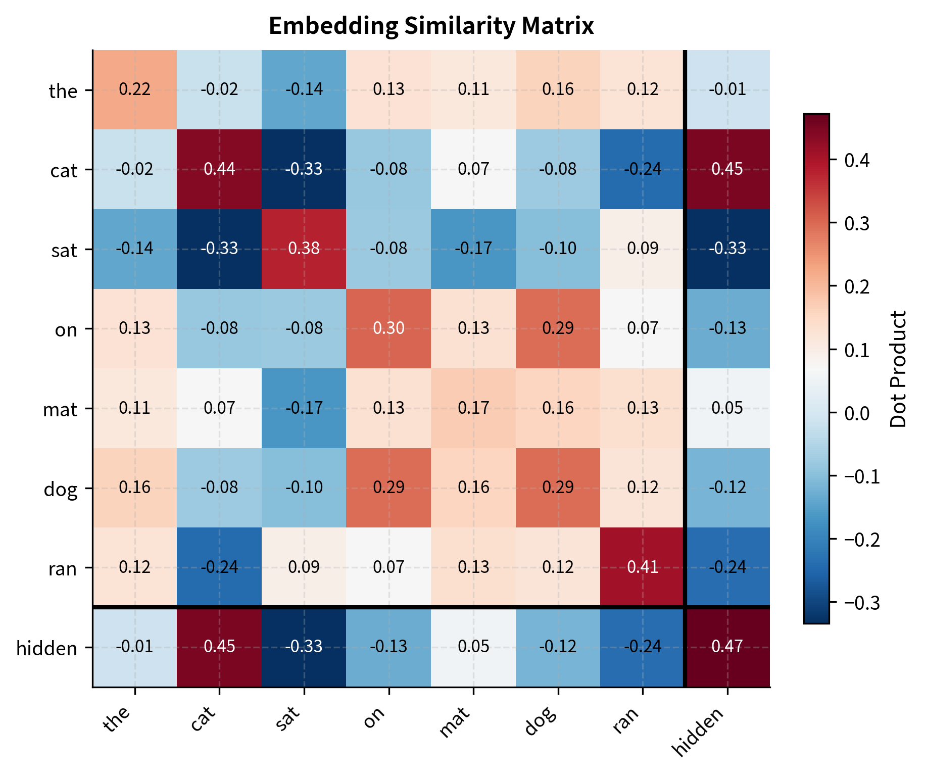
The heatmap reveals the structure of our embedding space. The bottom row (and rightmost column) shows how similar the hidden state is to each vocabulary embedding. Since we constructed the hidden state to resemble "cat", that cell shows the highest similarity in the hidden row. The diagonal entries are all positive because each embedding has positive self-similarity. Off-diagonal entries show how similar different tokens are to each other in the learned representation space.
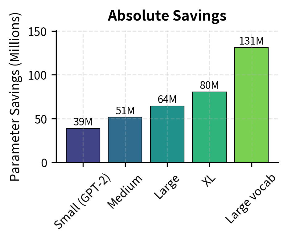
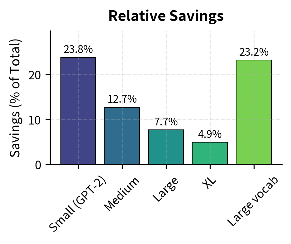
Scaling Considerations
Weight tying becomes more impactful as vocabulary size grows relative to model depth. Let's analyze how the savings scale:
For smaller models, weight tying can save 10-20% of total parameters. As models grow deeper, the relative savings decrease because transformer layers dominate, but the absolute parameter savings remain substantial.
To understand why weight tying matters more for some models than others, let's visualize how parameters are distributed:
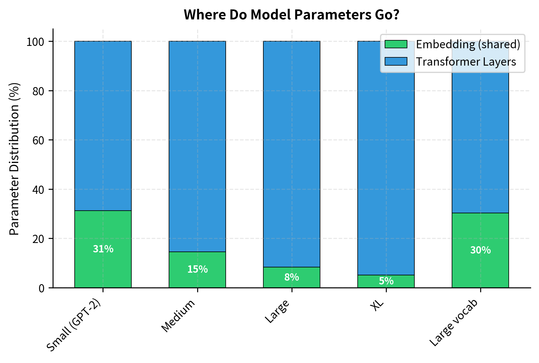
The visualization makes the trade-off clear. In GPT-2 Small, embeddings consume over 15% of parameters, so weight tying provides substantial savings. In the XL configuration, embeddings are less than 5% of the model. The "Large vocab" case is interesting: despite having more layers, the 128K vocabulary pushes embedding costs back up.
The "Large vocab" configuration shows an interesting pattern: models with bigger vocabularies (like those using 128K+ token vocabularies for multilingual support) benefit more from weight tying because the embedding matrix is a larger fraction of total parameters.
Encoder-Decoder Weight Tying
So far we've discussed tying input and output embeddings within a single model. Encoder-decoder architectures offer additional tying opportunities.
In a sequence-to-sequence model like T5 or BART, you have:
- Encoder input embeddings
- Decoder input embeddings
- Decoder output embeddings
Three separate matrices, all with the same shape , mapping between the same vocabulary and hidden dimension. Research has shown that tying all three together works well:
where:
- : the encoder input embedding matrix of shape
- : the decoder input embedding matrix of shape
- : the decoder output projection matrix of shape
- : the shared vocabulary size
- : the hidden dimension
This three-way tying means a single learned embedding serves all three roles: encoding source tokens, encoding target tokens during teacher forcing, and defining the output distribution over the vocabulary.
For encoder-decoder models, full weight tying eliminates two-thirds of embedding parameters. T5, one of the most successful encoder-decoder transformers, uses this three-way tying by default.
Effects on Training Dynamics
Weight tying doesn't just reduce parameters. It changes how the model learns.
Gradient Flow
With tied weights, the embedding matrix receives gradients from two sources:
- Input gradients: Backpropagated through the transformer from the loss
- Output gradients: Direct gradients from the output projection
This double gradient flow can be viewed as implicit multi-task learning. The embedding must simultaneously satisfy two objectives: representing tokens well for input processing, and providing good targets for output prediction.
The gradient magnitude shows how much the embedding weights would change in a single training step (before learning rate scaling). With tied weights, this gradient is typically larger than it would be with separate embeddings because it aggregates signals from both the input and output paths. This can speed up learning for rare tokens that might otherwise receive sparse gradient updates.
Embedding Scale
A subtle issue arises with weight tying: the optimal scale for input embeddings may differ from the optimal scale for output projections.
Input embeddings are often scaled by before being added to positional encodings (following the original transformer paper). The scaling factor is:
where:
- : the scaled input embedding
- : the embedding dimension
- : the raw embedding lookup for token
- : the scaling factor, which counterbalances the variance reduction that occurs when embeddings are initialized with small values
Without this scaling, embeddings initialized with small weights would be overwhelmed by positional encodings. But if we apply this scaling directly to the weight matrix, it would also affect the output logits when using tied weights, potentially making them too large.
Modern implementations handle this by applying scaling at input time rather than modifying the embedding matrix:
The scale factor of approximately 27.7 (for hidden dimension 768) significantly amplifies the input embeddings. By applying this scaling at runtime rather than baking it into the weights, we decouple the input and output requirements. The transformer processes scaled embeddings while the output projection uses raw embeddings, allowing each path to operate at its optimal scale.
When to Tie Weights
Weight tying isn't always the right choice. Here are the key considerations:
Tie weights when:
- Your vocabulary is large relative to model depth
- You want to reduce memory footprint without major architectural changes
- You're training from scratch and can let the model adapt
- Input and output domains are the same (e.g., language modeling)
Consider untied weights when:
- Input and output vocabularies differ (e.g., translation between different tokenizers)
- You're fine-tuning a pre-trained model that was trained without tying
- Model capacity is more important than parameter efficiency
- You observe that tied embeddings underperform in your specific task
The heuristic reveals an important pattern: smaller models like GPT-2 Small have embeddings that constitute a significant fraction of total parameters (over 15%), making weight tying highly impactful. For massive models like GPT-3 175B, embeddings are less than 1% of parameters, so tying provides minimal savings. However, even large models typically use weight tying because it rarely hurts performance and provides a small memory benefit. The multilingual translation case shows when tying is impossible: different input/output vocabularies require separate embedding spaces.
Limitations and Impact
Weight tying represents one of those elegant techniques where reducing complexity actually improves results. The constraint that input and output embeddings share the same learned representation forces the model to develop more coherent internal semantics.
The primary limitation is inflexibility. When input and output tasks require genuinely different token representations, tied weights create tension. Machine translation between languages with different scripts is the canonical example: the optimal encoding for reading Japanese may differ from the optimal target representation for generating English, even if both pass through the same vocabulary. In such cases, untied weights give the model freedom to specialize.
There's also a capacity argument. Very large models may benefit from the additional expressiveness of separate embeddings. When parameter count is less constrained, the regularization effect of tying matters less, and the model might learn better with independent representations. However, empirical evidence here is mixed, as even the largest models typically use tied weights.
Weight tying's impact extends beyond parameter efficiency. By forcing the model to reconcile input and output representations, it creates a more unified semantic space. This can improve generalization, especially for smaller models where every parameter must work harder. The technique has become standard practice in language modeling, appearing in GPT-2, BERT, T5, and most subsequent architectures. It's one of those design decisions that has become so universal that its presence is often assumed rather than stated.
Key Parameters
When implementing weight tying in your models, these are the key configuration choices:
-
tie_weights(bool): Whether to share the embedding matrix between input and output. Set toTruefor most language models; set toFalsewhen input and output vocabularies differ or when fine-tuning models trained without tying. -
vocab_size(int): Size of the vocabulary. Larger vocabularies increase the parameter savings from tying. With 50K+ tokens, embedding matrices can dominate smaller models. -
hidden_dim/d_model(int): The embedding and hidden dimension. This determines both the embedding matrix size () and the scale factor () used for input scaling. -
embedding_scale(float): Scaling factor applied to input embeddings, typically . Apply this at forward time rather than modifying the weight matrix to preserve unscaled embeddings for output projection. -
bias(bool): Whether to include a bias term in the output projection. Most implementations set this toFalsewhen using tied weights, as the embedding matrix provides sufficient expressivity.
Summary
Weight tying exploits the structural symmetry between input embedding and output projection matrices in language models. Both matrices have shape , where is vocabulary size and is the hidden dimension. Instead of maintaining separate matrices for input and for output, weight tying sets , so a single shared matrix serves both roles.
The key insights from this chapter:
-
Parameter reduction: Weight tying eliminates one full embedding matrix, saving parameters. For a 50K vocabulary with 768-dimensional embeddings, that's 38 million fewer parameters.
-
Theoretical justification: Input and output embeddings both answer "what does this token mean?" Tying them forces a consistent semantic representation where the hidden state that produces a token is similar to that token's embedding.
-
Implementation: The output projection becomes a matrix multiplication with the transposed embedding matrix. Gradients flow to the shared weights from both input and output paths.
-
Encoder-decoder extension: In sequence-to-sequence models, all three embedding matrices (encoder input, decoder input, decoder output) can share weights, eliminating two-thirds of embedding parameters.
-
Training effects: Tied weights receive gradients from multiple sources, creating implicit multi-task learning. Care must be taken with embedding scaling to handle different requirements for input and output.
-
When to use: Weight tying is recommended when vocabularies are large relative to model depth and input/output domains match. Avoid it when vocabularies differ or when maximum capacity is more important than efficiency.
Modern language models nearly universally adopt weight tying, making it a fundamental architectural decision rather than an optimization. Understanding why it works helps you reason about the semantic structure these models learn.
Quiz
Ready to test your understanding? Take this quick quiz to reinforce what you've learned about weight tying in language models.

Comments