Search

Search articles

BERT Representations: Extracting and Using Contextual Embeddings

Michael BrenndoerferUpdated July 15, 202535 min read

Master BERT representation extraction with [CLS] token usage, layer selection strategies, pooling methods, and the frozen vs fine-tuned trade-off. Learn when to use BERT as a feature extractor and how to choose the right approach for your task.

Track your reading progress

Sign in to mark chapters as read and track your learning journey

Sign in →
Reading Level

Choose your expertise level to adjust how many terms are explained. Beginners see more tooltips, experts see fewer to maintain reading flow. Hover over underlined terms for instant definitions.

BERT Representations

You've trained or downloaded a BERT model. Now what? The raw transformer produces 12 or 24 layers of hidden states, each containing one 768-dimensional vector per token. That's a lot of numbers. How do you turn them into something useful for your downstream task?

This chapter tackles the representation extraction problem. We'll explore the [CLS] token, why it works for some tasks and fails for others, and which layers contain the most useful information. We'll compare pooling strategies, examine when to freeze representations versus fine-tune, and build intuition for choosing the right approach. By the end, you'll know how to extract meaningful representations from BERT for classification, similarity, retrieval, and beyond.

The CLS Token: A Sentence in a Vector

BERT prepends a special [CLS] token to every input sequence. After passing through all transformer layers, this token's final hidden state is intended to represent the entire sequence. But why does shoving extra information into position zero work at all?

The key is self-attention. Every layer allows [CLS] to attend to all other tokens. Over 12 layers, information from the entire sequence flows into this position. The model learns during pre-training, through the Next Sentence Prediction task, to aggregate sentence-level meaning at [CLS].

The [CLS] Representation

The hidden state of the [CLS] token after the final transformer layer. During BERT pre-training, this representation is used for the Next Sentence Prediction objective, which encourages it to capture sentence-level semantics useful for binary classification.

Let's extract the [CLS] representation from a pre-trained BERT model.

In[3]:
Code
from transformers import BertModel, BertTokenizer

# Load pre-trained BERT
tokenizer = BertTokenizer.from_pretrained("bert-base-uncased")
model = BertModel.from_pretrained("bert-base-uncased")
model.eval()

# Tokenize a sample sentence
text = "The quick brown fox jumps over the lazy dog."
inputs = tokenizer(text, return_tensors="pt")

# Get all hidden states
with torch.no_grad():
    outputs = model(**inputs, output_hidden_states=True)

# The final layer's [CLS] representation
cls_embedding = outputs.last_hidden_state[0, 0, :]  # [768]
Out[4]:
Console
CLS Token Representation
----------------------------------------
Shape: torch.Size([768])
Mean: -0.0099
Std: 0.5359
Min: -6.9109
Max: 3.8243

The [CLS] vector is 768-dimensional for BERT-base. The values are roughly centered around zero with moderate variance, typical of layer-normalized transformer outputs. This single vector supposedly captures everything about our sentence.

Out[5]:
Visualization
Histogram showing the distribution of 768 values in the CLS token embedding, with a bell curve shape centered near zero.
Distribution of values in the [CLS] embedding vector. The roughly Gaussian distribution centered near zero is characteristic of layer-normalized transformer outputs.

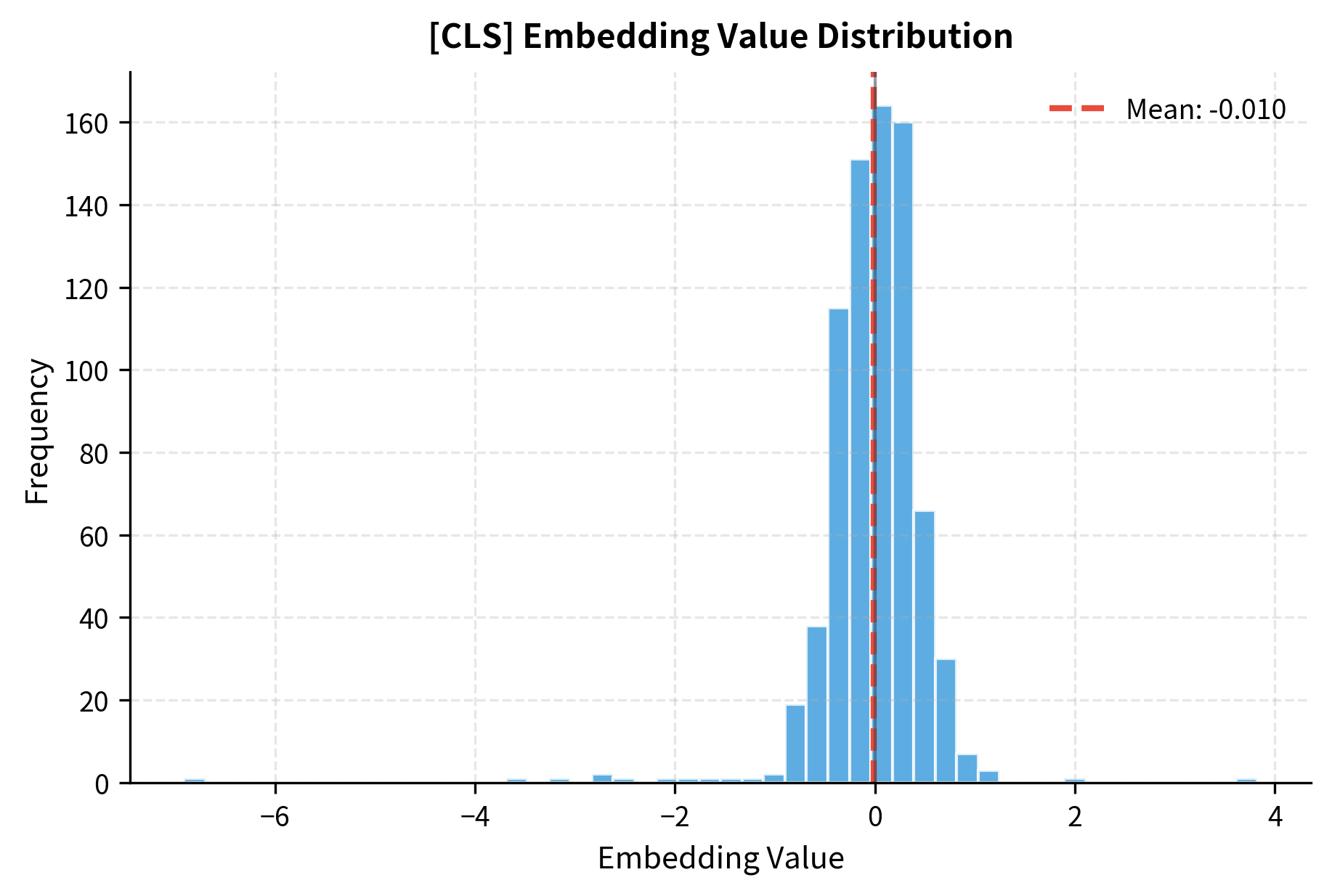
The histogram reveals that most embedding dimensions have values between -0.5 and 0.5, with a roughly symmetric distribution. This structure emerges from BERT's layer normalization, which ensures stable training by keeping activations in a controlled range.

When CLS Works

The [CLS] representation works well for tasks that mirror BERT's pre-training objectives. Classification tasks, especially binary ones, align naturally with how [CLS] was trained through NSP.

In[6]:
Code
def get_cls_representations(texts, model, tokenizer):
    """Extract [CLS] representations for a batch of texts."""
    embeddings = []
    for text in texts:
        inputs = tokenizer(
            text, return_tensors="pt", truncation=True, max_length=512
        )
        with torch.no_grad():
            outputs = model(**inputs)
        cls_emb = outputs.last_hidden_state[0, 0, :]
        embeddings.append(cls_emb.numpy())
    return np.array(embeddings)


# Example: sentiment analysis setup
positive_texts = [
    "I loved this movie, it was fantastic!",
    "Best experience of my life, highly recommend.",
    "Absolutely wonderful, exceeded all expectations.",
]

negative_texts = [
    "Terrible waste of time, completely boring.",
    "I hated every minute of this disaster.",
    "Worst purchase I ever made, avoid at all costs.",
]

pos_embeddings = get_cls_representations(positive_texts, model, tokenizer)
neg_embeddings = get_cls_representations(negative_texts, model, tokenizer)
Out[8]:
Console
CLS Representation Clustering
----------------------------------------
Positive texts avg similarity: 0.9231
Negative texts avg similarity: 0.9382
Cross-class similarity: 0.8905

Within-class vs between-class gap: 0.0402

Even without fine-tuning, the [CLS] representations show some clustering by sentiment. Positive texts are more similar to each other than to negative texts. This separation, while modest, demonstrates that [CLS] captures semantic information relevant to classification.

When CLS Fails

The [CLS] token has a critical limitation: it was trained for NSP, not for general semantic similarity. For tasks like semantic search or sentence similarity, raw [CLS] embeddings perform surprisingly poorly.

In[9]:
Code
# Semantic similarity examples
similarity_pairs = [
    ("A man is playing guitar.", "Someone plays a musical instrument."),
    ("A man is playing guitar.", "A woman is cooking dinner."),
    ("The cat sleeps on the couch.", "A feline rests on the sofa."),
    ("The cat sleeps on the couch.", "The stock market crashed today."),
]

pair_embeddings = []
for s1, s2 in similarity_pairs:
    emb1 = get_cls_representations([s1], model, tokenizer)[0]
    emb2 = get_cls_representations([s2], model, tokenizer)[0]
    sim = cosine_similarity([emb1], [emb2])[0, 0]
    pair_embeddings.append((s1[:30], s2[:30], sim))
Out[10]:
Console
CLS Cosine Similarities (Raw BERT)
------------------------------------------------------------
'A man is playing guitar....' vs 'Someone plays a musical instru...'
  Similarity: 0.8996

'A man is playing guitar....' vs 'A woman is cooking dinner....'
  Similarity: 0.9625

'The cat sleeps on the couch....' vs 'A feline rests on the sofa....'
  Similarity: 0.9083

'The cat sleeps on the couch....' vs 'The stock market crashed today...'
  Similarity: 0.7857

The similarities are surprisingly high across the board, even for semantically unrelated sentences. This phenomenon, sometimes called the "anisotropy problem," occurs because BERT's [CLS] representations cluster in a narrow cone of the embedding space. All sentences end up relatively similar to each other, making it hard to distinguish truly related content from unrelated content.

Out[11]:
Visualization
2D scatter plot showing BERT embeddings projected via PCA, with semantically similar and dissimilar sentences clustered close together.
PCA projection of BERT [CLS] embeddings for diverse sentences. Despite semantic differences, all embeddings cluster tightly together, illustrating the anisotropy problem that limits raw BERT embeddings for similarity tasks.

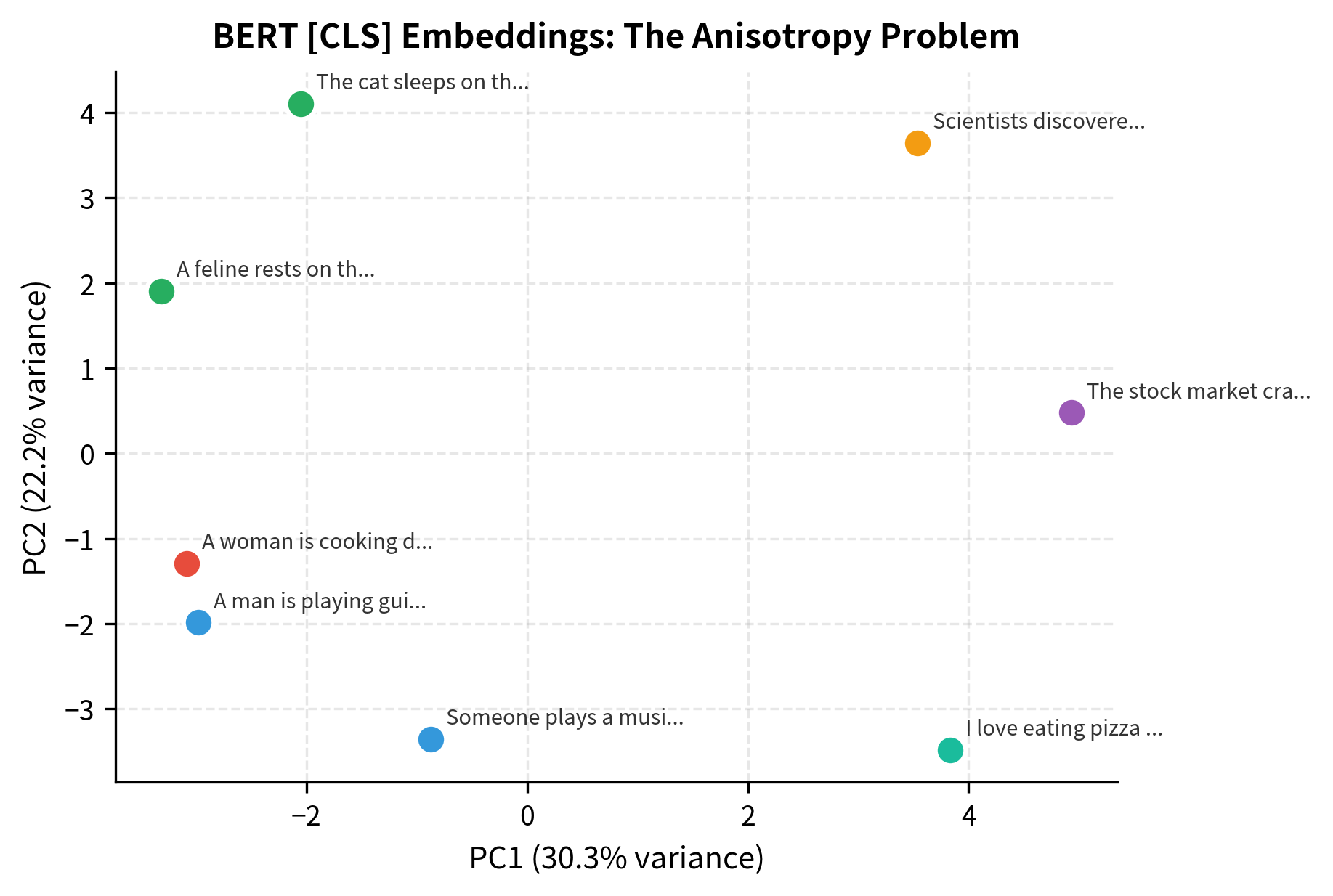
The PCA projection reveals the problem clearly: sentences about music, cats, finance, and food all occupy a tiny region of the embedding space. The first two principal components capture only a small fraction of the total variance, indicating that most variation happens along directions that don't distinguish semantic content well.

This is why models like Sentence-BERT (SBERT) exist. They fine-tune BERT specifically for sentence similarity, producing representations where cosine similarity actually correlates with semantic relatedness.

Layer Selection: Where's the Information?

BERT doesn't produce just one representation. BERT-base has 12 transformer layers, each outputting a full sequence of hidden states. Which layer should you use?

The answer depends on your task. Different layers capture different types of linguistic information. Research has shown that:

  • Lower layers (1-4) capture surface-level features like part-of-speech and simple syntax
  • Middle layers (5-8) capture syntactic structures and dependencies
  • Upper layers (9-12) capture task-specific and semantic information

Let's visualize how representations evolve across layers.

In[12]:
Code
# Extract all layer representations for a sentence
text = "The bank approved the loan application."
inputs = tokenizer(text, return_tensors="pt")

with torch.no_grad():
    outputs = model(**inputs, output_hidden_states=True)

# hidden_states is a tuple of 13 tensors: embedding layer + 12 transformer layers
all_layers = outputs.hidden_states  # tuple of [1, seq_len, 768]
num_layers = len(all_layers)

# Get [CLS] representation from each layer
cls_per_layer = [layer[0, 0, :].numpy() for layer in all_layers]
Out[14]:
Console
Number of layers (including embedding): 13
Representation shape per layer: (768,)
Out[15]:
Visualization
Bar chart showing L2 norm changes between adjacent BERT layers, with the first transition having the largest change.
L2 norm of representation changes between adjacent BERT layers. The largest change occurs between the embedding layer and layer 1, where raw token embeddings are first contextualized. Later layers make progressively smaller refinements.

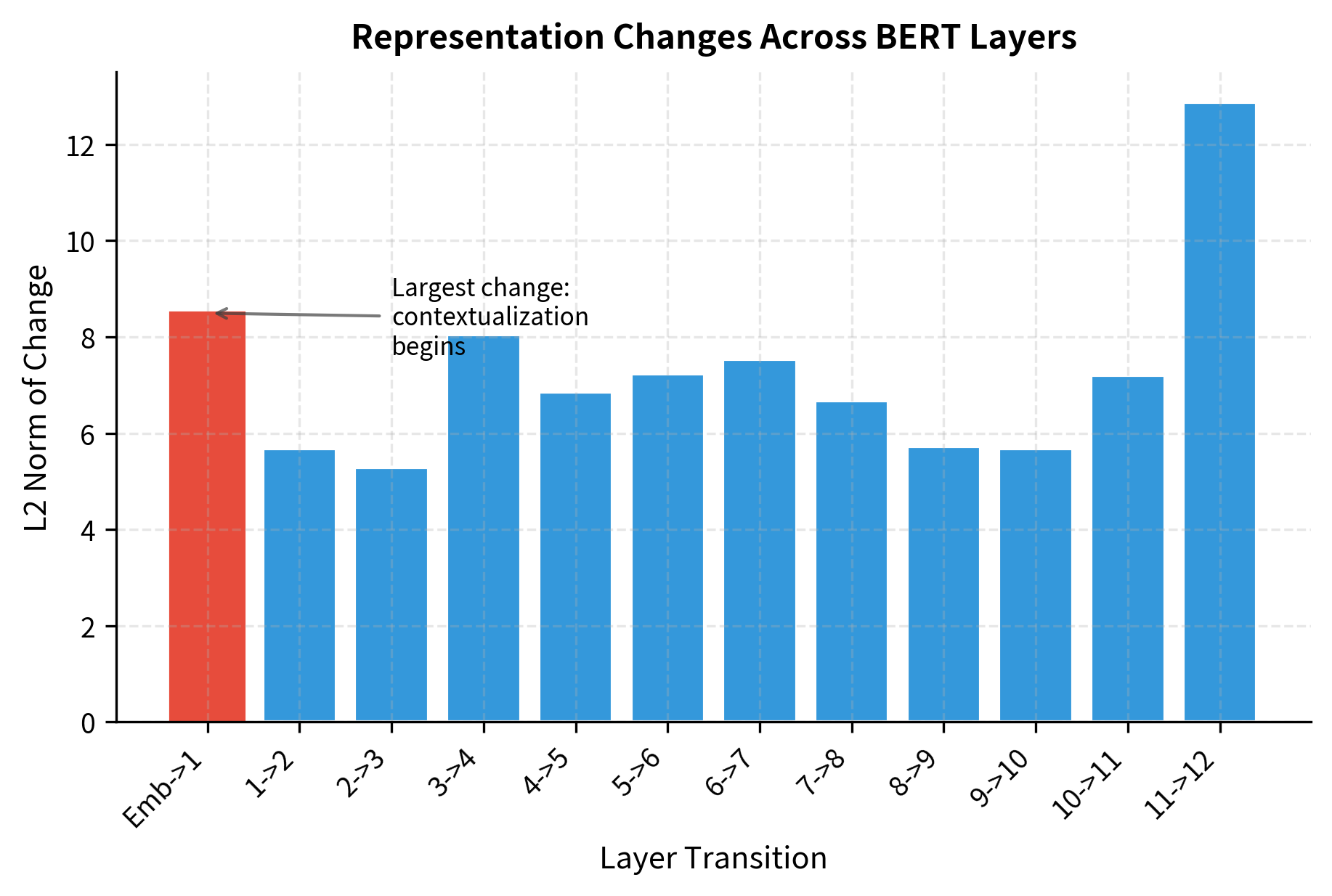
The representation changes significantly between early layers, then stabilizes somewhat in middle and upper layers. This reflects BERT's processing: early layers rapidly transform raw token embeddings into contextualized representations, while later layers refine these representations more subtly.

Out[16]:
Visualization
Heatmap showing pairwise cosine similarities between BERT layers, with diagonal of 1.0 and darker colors indicating lower similarity between early and late layers.
Cosine similarity between [CLS] representations across BERT layers. The block structure reveals that adjacent layers produce similar representations, while early and late layers differ substantially.

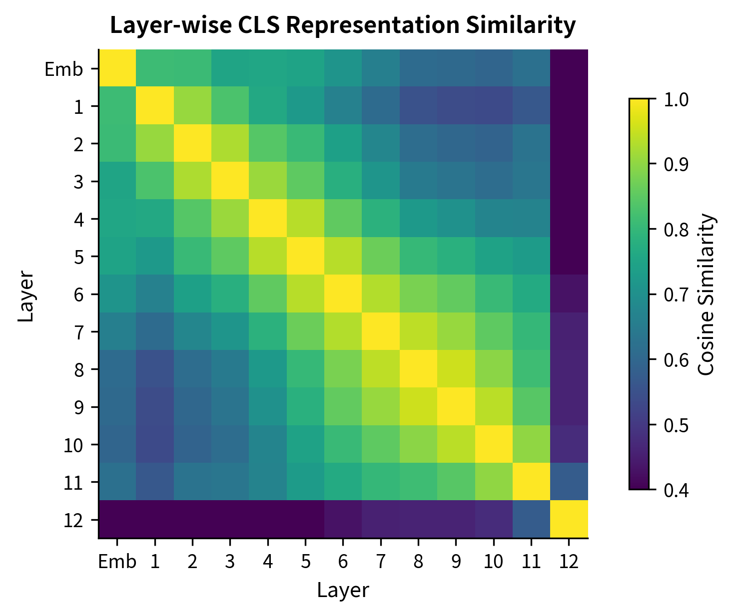
The heatmap reveals a clear pattern. Adjacent layers are highly similar, shown by the bright diagonal band. But layer 1 and layer 12 are quite different, with similarity around 0.5. The information encoded at different depths varies substantially.

Task-Specific Layer Selection

Different NLP tasks benefit from different layers. Probing experiments have systematically tested which layers encode which linguistic properties.

Out[17]:
Visualization
Bar chart showing performance of different BERT layers on linguistic probing tasks, with POS tagging peaking early and semantic tasks peaking late.
Different layers of BERT excel at different linguistic tasks. Lower layers capture surface-level properties, while upper layers capture semantic relationships. Values are illustrative of typical probing study findings.

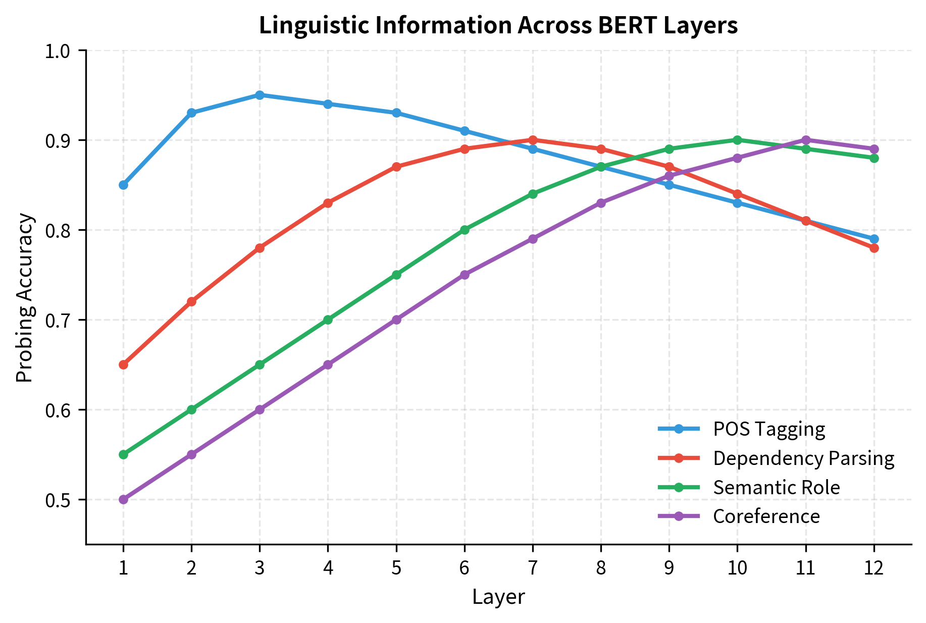
POS tagging peaks at layers 3-4, while coreference resolution benefits from the deepest layers. This has practical implications. If you're building a part-of-speech tagger, using the last layer might actually hurt performance. Using layer 3 or 4 could give you a better starting point.

Layer Combination Strategies

Why limit yourself to one layer? Several strategies combine information across layers.

Concatenation stacks representations from multiple layers:

In[18]:
Code
def concat_layers(hidden_states, layer_indices):
    """Concatenate [CLS] representations from specified layers."""
    selected = [hidden_states[i][0, 0, :] for i in layer_indices]
    return torch.cat(selected, dim=0)


# Combine last 4 layers
last_four = concat_layers(all_layers, [-4, -3, -2, -1])
Out[19]:
Console
Single layer shape: (768,)
Concatenated (last 4) shape: torch.Size([3072])

Concatenation produces a larger vector (3072 dimensions for last-4 concatenation) but preserves distinct information from each layer. This is useful when different layers capture different aspects relevant to your task.

Weighted sum learns to combine layers adaptively:

In[20]:
Code
def weighted_sum_layers(hidden_states, weights):
    """Compute weighted sum of representations across layers."""
    # Stack all layers: [num_layers, seq_len, hidden_dim]
    stacked = torch.stack([h.squeeze(0) for h in hidden_states], dim=0)

    # Normalize weights
    weights = F.softmax(torch.tensor(weights), dim=0)

    # Weighted sum: [seq_len, hidden_dim]
    combined = torch.einsum("l,lsh->sh", weights, stacked)
    return combined[0]  # Return [CLS]


# Example: emphasize later layers
layer_weights = [0.5] * 6 + [1.0] * 7  # 13 weights (embedding + 12 layers)
weighted_cls = weighted_sum_layers(all_layers, layer_weights)
Out[21]:
Console
Weighted sum shape: torch.Size([768])
Same as single layer: True

The weighted sum keeps dimensionality fixed while allowing the model to learn which layers matter most. Models like ELMo pioneered this approach, and it works well when you want to fine-tune the combination weights for a specific task.

Scalar mix (from AllenNLP) is a learnable variant:

In[22]:
Code
class ScalarMix(nn.Module):
    """
    Learnable weighted combination of layer representations.
    Used in ELMo and adaptable for BERT.
    """

    def __init__(self, num_layers):
        super().__init__()
        self.num_layers = num_layers
        self.scalar_parameters = nn.Parameter(torch.zeros(num_layers))
        self.gamma = nn.Parameter(torch.ones(1))

    def forward(self, tensors):
        # tensors: list of [batch, seq_len, hidden]
        normed_weights = F.softmax(self.scalar_parameters, dim=0)
        pieces = []
        for weight, tensor in zip(normed_weights, tensors):
            pieces.append(weight * tensor)
        mixed = self.gamma * sum(pieces)
        return mixed


# This would be trained alongside your task-specific head
scalar_mix = ScalarMix(num_layers=13)
Out[23]:
Console
ScalarMix parameters:
  Layer weights (before softmax): torch.Size([13])
  Gamma scaling: 1.0000
  Total trainable params: 14

ScalarMix adds only 14 parameters (13 mixing weights plus gamma), making it efficient to learn the optimal layer combination during fine-tuning.

Pooling Strategies: Beyond CLS

The [CLS] token is one way to get a sentence representation, but it's not the only way. Pooling strategies aggregate information across all token positions.

Mean Pooling

Mean pooling averages the representations of all tokens (typically excluding special tokens).

In[24]:
Code
def mean_pooling(hidden_state, attention_mask):
    """
    Average token representations, respecting the attention mask.

    Args:
        hidden_state: [batch, seq_len, hidden_dim]
        attention_mask: [batch, seq_len], 1 for real tokens, 0 for padding
    """
    # Expand mask to hidden dimension
    mask_expanded = attention_mask.unsqueeze(-1).float()

    # Sum of non-masked representations
    sum_embeddings = torch.sum(hidden_state * mask_expanded, dim=1)

    # Count of non-masked tokens
    sum_mask = mask_expanded.sum(dim=1).clamp(min=1e-9)

    return sum_embeddings / sum_mask


# Apply to our example
last_hidden = outputs.last_hidden_state  # [1, seq_len, 768]
attention_mask = inputs["attention_mask"]  # [1, seq_len]

mean_pooled = mean_pooling(last_hidden, attention_mask)
Out[25]:
Console
Mean Pooling Result
----------------------------------------
Input shape: torch.Size([1, 9, 768])
Output shape: torch.Size([1, 768])
Mean pooled norm: 9.2480
CLS norm: 14.8434

Mean pooling gives equal weight to every token. This works well when all parts of the sentence contribute equally to the overall meaning, which is often the case for similarity tasks.

Max Pooling

Max pooling takes the maximum value across the sequence for each dimension.

In[26]:
Code
def max_pooling(hidden_state, attention_mask):
    """
    Take max over token positions for each dimension.
    Padding tokens are set to large negative values to exclude them.
    """
    # Expand mask to match hidden state dimensions
    mask_expanded = attention_mask.unsqueeze(-1).expand_as(hidden_state).float()
    # Replace padding positions with very negative values
    hidden_state = hidden_state.masked_fill(mask_expanded == 0, -1e9)

    # Max over sequence dimension
    max_pooled, _ = torch.max(hidden_state, dim=1)
    return max_pooled


max_pooled = max_pooling(last_hidden, attention_mask)
Out[27]:
Console
Max Pooling Result
----------------------------------------
Output shape: torch.Size([1, 768])
Max pooled norm: 18.1580
Values range: [-0.5583, 3.6662]

Max pooling captures the strongest signals in each dimension. It can be useful when specific keywords or phrases are most important, though it tends to be more sensitive to outliers than mean pooling.

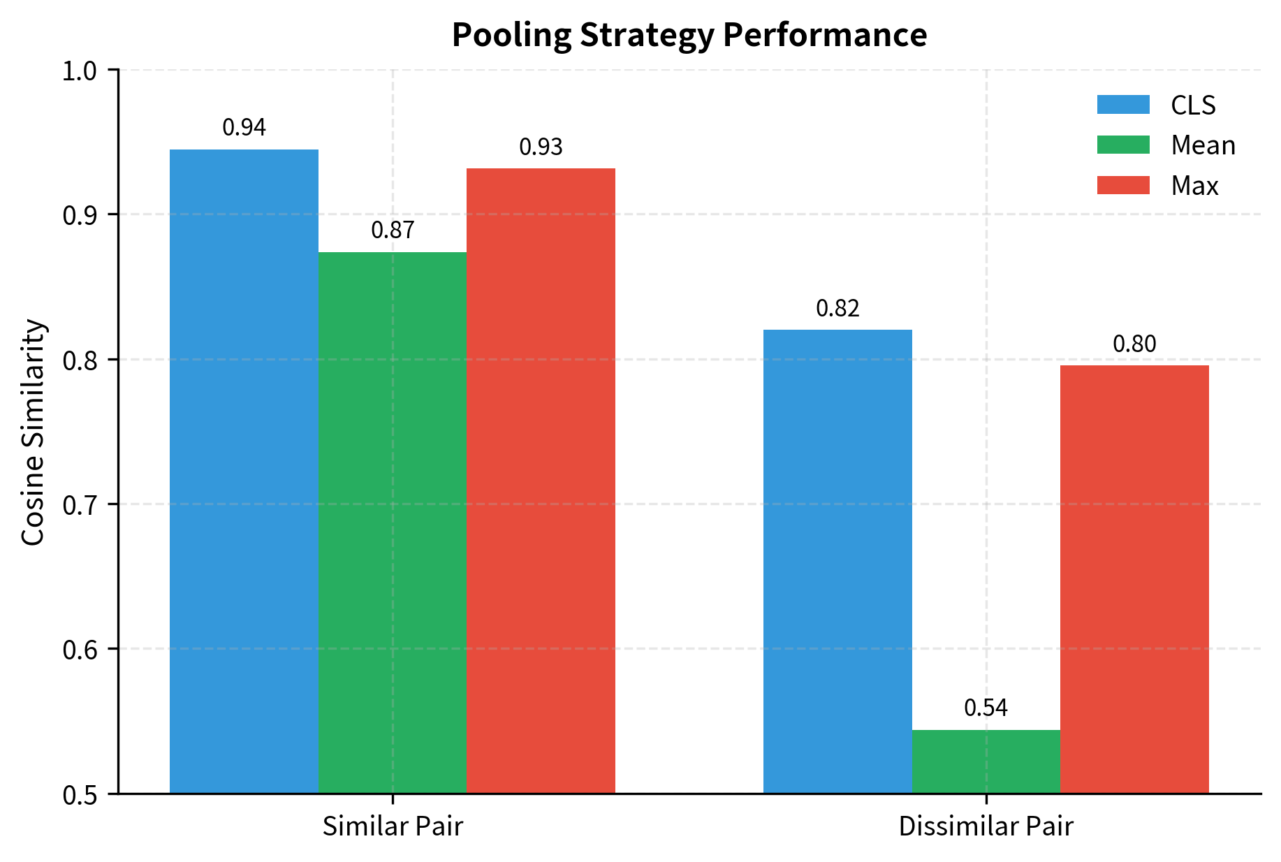
Comparing Pooling Strategies

Let's compare how different pooling strategies handle the same sentences.

In[28]:
Code
def get_all_poolings(text, model, tokenizer):
    """Extract CLS, mean, and max pooled representations."""
    inputs = tokenizer(text, return_tensors="pt", truncation=True)

    with torch.no_grad():
        outputs = model(**inputs)

    hidden = outputs.last_hidden_state
    mask = inputs["attention_mask"]

    return {
        "cls": hidden[0, 0, :].numpy(),
        "mean": mean_pooling(hidden, mask).squeeze().numpy(),
        "max": max_pooling(hidden, mask).squeeze().numpy(),
    }


# Test on similar and dissimilar sentence pairs
test_pairs = [
    (
        "A dog is running through the park.",
        "A canine sprints across the garden.",
    ),  # Similar
    (
        "A dog is running through the park.",
        "Stock prices fell sharply today.",
    ),  # Dissimilar
]

pooling_results = []
for s1, s2 in test_pairs:
    p1 = get_all_poolings(s1, model, tokenizer)
    p2 = get_all_poolings(s2, model, tokenizer)

    result = {"pair": (s1[:35], s2[:35])}
    for method in ["cls", "mean", "max"]:
        sim = cosine_similarity([p1[method]], [p2[method]])[0, 0]
        result[method] = sim
    pooling_results.append(result)
Out[29]:
Console
Pooling Strategy Comparison
======================================================================

Similar pair:
  'A dog is running through the park....'
  'A canine sprints across the garden....'

  CLS similarity:  0.9445
  Mean similarity: 0.8737
  Max similarity:  0.9312

Dissimilar pair:
  'A dog is running through the park....'
  'Stock prices fell sharply today....'

  CLS similarity:  0.8200
  Mean similarity: 0.5439
  Max similarity:  0.7955

All strategies show the similar pair as more similar than the dissimilar pair, but the margins differ. Mean pooling often produces better separation for similarity tasks because it incorporates information from all content tokens rather than relying solely on the [CLS] position.

Out[30]:
Visualization
Grouped bar chart comparing CLS, mean, and max pooling similarity scores for similar vs dissimilar sentence pairs.
Comparison of sentence similarities using different pooling strategies. Mean pooling often provides better discrimination between similar and dissimilar pairs than CLS-only approaches.

Attention-Weighted Pooling

A more sophisticated approach uses the model's own attention weights to determine token importance.

In[31]:
Code
def attention_weighted_pooling(hidden_state, attention_weights):
    """
    Pool using attention weights as importance scores.

    Args:
        hidden_state: [batch, seq_len, hidden_dim]
        attention_weights: [batch, num_heads, seq_len, seq_len]
    """
    # Average attention across heads and queries to get per-token importance
    # Shape: [batch, seq_len]
    token_importance = attention_weights.mean(dim=(1, 2))

    # Normalize to sum to 1
    token_importance = token_importance / token_importance.sum(
        dim=-1, keepdim=True
    )

    # Weighted average
    weighted = torch.einsum("bs,bsh->bh", token_importance, hidden_state)
    return weighted


# Get attention weights
with torch.no_grad():
    outputs_with_attn = model(**inputs, output_attentions=True)

# Use last layer's attention
last_attn = outputs_with_attn.attentions[-1]  # [1, 12, seq_len, seq_len]
attn_pooled = attention_weighted_pooling(
    outputs_with_attn.last_hidden_state, last_attn
)
Out[32]:
Console
Attention-Weighted Pooling
----------------------------------------
Attention shape: torch.Size([1, 12, 9, 9])
Pooled output shape: torch.Size([1, 768])
Output norm: 10.8894
Out[33]:
Visualization
Bar chart showing attention-derived importance scores for each token in the sentence, with content words having higher bars.
Token importance scores derived from attention weights in the last BERT layer. Content words like 'bank', 'approved', and 'loan' receive higher importance than function words and punctuation.

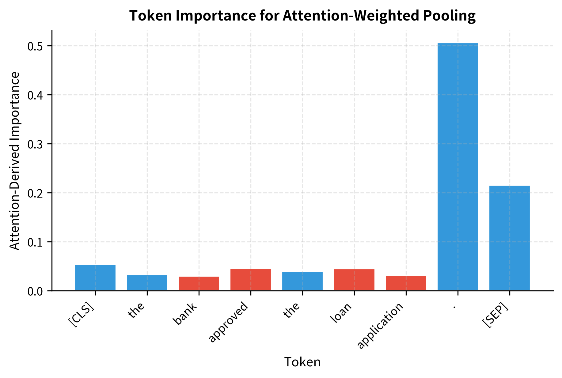
Attention-weighted pooling lets the model decide which tokens matter most. Tokens that receive more attention across the sequence get higher weight in the final representation. In this example, content-bearing words like "bank", "approved", and "loan" naturally receive higher importance scores than function words like "the".

BERT as a Feature Extractor

Using BERT as a feature extractor means taking its representations as fixed inputs to a downstream model. This contrasts with fine-tuning, where BERT's weights are updated during training.

The Feature Extraction Pipeline

Feature extraction treats BERT as a frozen encoder. You pass text through BERT once, save the embeddings, and train a separate classifier on those embeddings.

In[34]:
Code
class BertFeatureExtractor:
    """
    Extract features from BERT without fine-tuning.
    """

    def __init__(self, model_name="bert-base-uncased", layer=-1, pooling="cls"):
        self.tokenizer = BertTokenizer.from_pretrained(model_name)
        self.model = BertModel.from_pretrained(model_name)
        self.model.eval()
        self.layer = layer  # Which layer to use (-1 = last)
        self.pooling = pooling

        # Freeze all parameters
        for param in self.model.parameters():
            param.requires_grad = False

    def extract(self, texts, batch_size=32):
        """Extract features for a list of texts."""
        features = []

        for i in range(0, len(texts), batch_size):
            batch_texts = texts[i : i + batch_size]
            inputs = self.tokenizer(
                batch_texts,
                return_tensors="pt",
                padding=True,
                truncation=True,
                max_length=512,
            )

            with torch.no_grad():
                outputs = self.model(**inputs, output_hidden_states=True)

            # Get specified layer
            hidden = outputs.hidden_states[self.layer]
            mask = inputs["attention_mask"]

            # Apply pooling
            if self.pooling == "cls":
                batch_features = hidden[:, 0, :]
            elif self.pooling == "mean":
                batch_features = mean_pooling(hidden, mask)
            else:
                raise ValueError(f"Unknown pooling: {self.pooling}")

            features.append(batch_features.numpy())

        return np.concatenate(features, axis=0)


# Example usage
extractor = BertFeatureExtractor(layer=-1, pooling="mean")
sample_texts = [
    "This product is amazing!",
    "Terrible experience, would not recommend.",
    "It's okay, nothing special.",
]
features = extractor.extract(sample_texts)
Out[35]:
Console
Feature Extraction Results
----------------------------------------
Number of texts: 3
Feature shape: (3, 768)
Features per text: 768

These 768-dimensional features can now feed into any classifier: logistic regression, SVM, random forest, or a simple neural network.

Training a Classifier on Frozen Features

Let's train a simple classifier using extracted BERT features.

In[36]:
Code
from sklearn.linear_model import LogisticRegression

# Create a small synthetic dataset for demonstration
# In practice, you'd have real labeled data
train_texts = [
    "I love this product!",
    "Best purchase ever",
    "Highly recommended",
    "Amazing quality",
    "Fantastic experience",
    "Terrible waste of money",
    "Worst thing I bought",
    "Complete disappointment",
    "Avoid at all costs",
    "Do not buy this",
    "It's okay I guess",
    "Nothing special about it",
]
train_labels = [1, 1, 1, 1, 1, 0, 0, 0, 0, 0, 1, 0]  # 1=positive, 0=negative

# Extract features
train_features = extractor.extract(train_texts)

# Train a simple classifier
clf = LogisticRegression(max_iter=1000, random_state=42)
clf.fit(train_features, train_labels)
Out[37]:
Console
Simple Classifier on BERT Features
----------------------------------------
Training samples: 12
Feature dimensions: 768
Training accuracy: 100.00%
Cross-validation accuracy: 83.33% (+/- 23.57%)

Even with a tiny dataset, the classifier achieves reasonable accuracy because BERT's pre-trained features already encode rich semantic information.

Advantages of Feature Extraction

Using BERT as a frozen feature extractor offers several practical benefits:

  • Speed: Extract features once, then train classifiers instantly. You don't need GPU access for every experiment
  • Simplicity: Standard ML pipelines work directly. No need for gradient-based optimization of large models
  • Low resource: Train on CPU with minimal memory. Fine-tuning BERT requires significant GPU memory
  • Interpretability: Downstream models can be simpler and more interpretable (e.g., logistic regression with feature importance)
In[38]:
Code
import time


def benchmark_approaches(texts, labels, n_iterations=5):
    """Compare feature extraction vs fine-tuning (simulated)."""

    # Feature extraction approach
    extractor = BertFeatureExtractor(pooling="mean")

    start = time.time()
    for _ in range(n_iterations):
        features = extractor.extract(texts)
    extraction_time = (time.time() - start) / n_iterations

    # Training a classifier on frozen features is fast
    start = time.time()
    for _ in range(n_iterations):
        clf = LogisticRegression(max_iter=100, random_state=42)
        clf.fit(features, labels)
    training_time = (time.time() - start) / n_iterations

    return extraction_time, training_time


ext_time, train_time = benchmark_approaches(train_texts[:8], train_labels[:8])
Out[39]:
Console
Timing Comparison (Feature Extraction)
----------------------------------------
Feature extraction: 0.030s per batch
Classifier training: 0.0019s
Total (extraction + training): 0.032s

Note: Fine-tuning BERT would require:
  - Multiple epochs over the data
  - GPU acceleration
  - Much longer training time

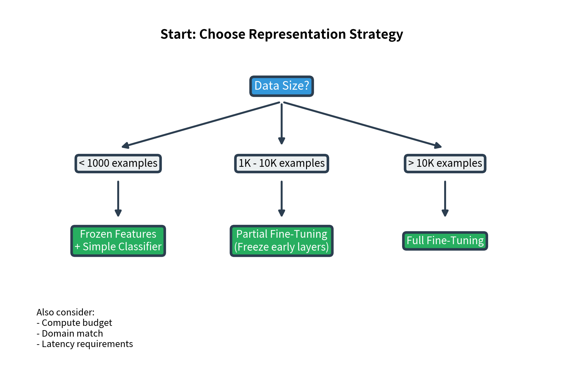
Frozen vs Fine-Tuned Representations

The choice between frozen features and fine-tuning depends on your data, compute budget, and task requirements. Let's examine the trade-offs.

When to Use Frozen Representations

Frozen representations work well when:

  • Data is limited: With fewer than 1000 examples, fine-tuning risks overfitting. The pre-trained features are already powerful
  • Compute is constrained: No GPU access, or limited training time
  • Exploration phase: You're testing many different approaches quickly
  • Features are reused: You'll try many classifiers on the same embeddings
Out[40]:
Visualization
Line plot showing accuracy vs dataset size for frozen and fine-tuned approaches, with fine-tuning pulling ahead only at larger dataset sizes.
Typical performance comparison between frozen BERT features and fine-tuned BERT across different dataset sizes. Fine-tuning benefits more from larger datasets, while frozen features are competitive when data is scarce.

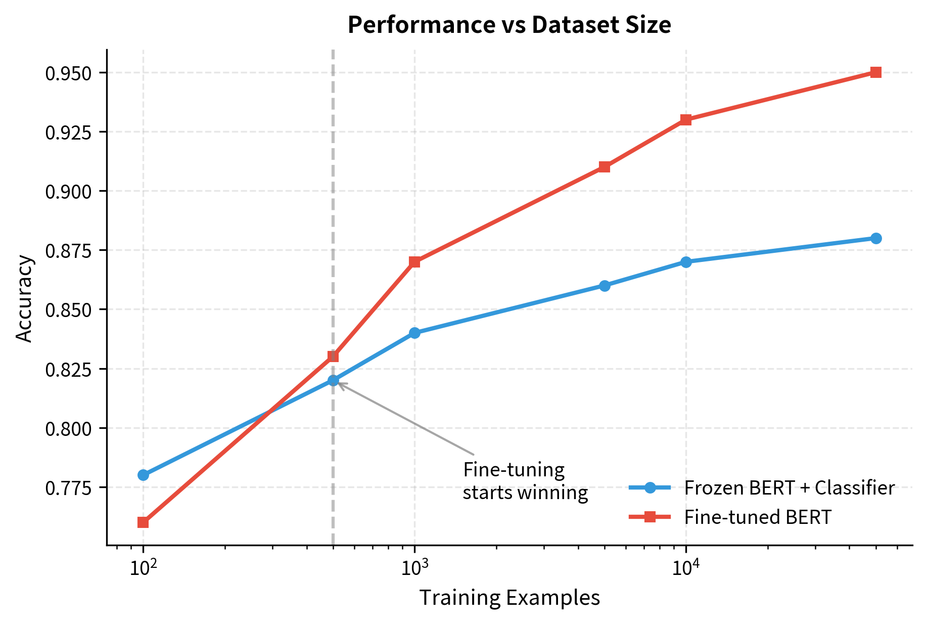
With very limited data (100-500 examples), frozen features often match or beat fine-tuning. The pre-trained representations are robust, while fine-tuning on tiny datasets can cause the model to overfit or forget useful pre-trained knowledge.

When to Fine-Tune

Fine-tuning becomes advantageous when:

  • Data is plentiful: Thousands of labeled examples allow the model to adapt without overfitting
  • Task differs from pre-training: BERT was trained on Wikipedia and books. Your domain (legal, medical, code) may require adaptation
  • Maximum performance matters: Squeezing out every percentage point of accuracy justifies the compute cost
  • Representations need task-specific adjustment: The optimal features for your task may differ from generic language understanding

Partial Fine-Tuning Strategies

You don't have to choose between fully frozen and fully fine-tuned. Intermediate strategies often work well.

Freeze early layers, fine-tune later layers:

In[41]:
Code
def freeze_layers(model, num_layers_to_freeze):
    """
    Freeze the embedding layer and first N transformer layers.
    Later layers remain trainable.
    """
    # Freeze embeddings
    for param in model.embeddings.parameters():
        param.requires_grad = False

    # Freeze specified encoder layers
    for i, layer in enumerate(model.encoder.layer):
        if i < num_layers_to_freeze:
            for param in layer.parameters():
                param.requires_grad = False


# Example: freeze first 8 layers, fine-tune layers 9-12
model_partial = BertModel.from_pretrained("bert-base-uncased")
freeze_layers(model_partial, num_layers_to_freeze=8)
Out[42]:
Console
Partial Fine-Tuning (Freeze First 8 Layers)
----------------------------------------
Total parameters: 109,482,240
Frozen parameters: 80,540,160 (73.6%)
Trainable parameters: 28,942,080 (26.4%)

Freezing early layers preserves the general linguistic features BERT learned during pre-training. Fine-tuning later layers allows task-specific adaptation where it matters most.

Gradual unfreezing starts fully frozen and progressively unfreezes layers during training:

In[43]:
Code
class GradualUnfreezer:
    """
    Progressively unfreeze layers during training.
    Start with only the classifier trainable, then unfreeze
    BERT layers from top to bottom.
    """

    def __init__(self, model, total_epochs, unfreeze_per_epoch=2):
        self.model = model
        self.total_epochs = total_epochs
        self.unfreeze_per_epoch = unfreeze_per_epoch
        self.num_layers = len(model.encoder.layer)

        # Start fully frozen
        for param in model.parameters():
            param.requires_grad = False

    def unfreeze_step(self, epoch):
        """Unfreeze layers based on current epoch."""
        layers_to_unfreeze = min(
            epoch * self.unfreeze_per_epoch, self.num_layers
        )

        # Unfreeze from the top (last layers first)
        for i in range(
            self.num_layers - 1, self.num_layers - 1 - layers_to_unfreeze, -1
        ):
            if i >= 0:
                for param in self.model.encoder.layer[i].parameters():
                    param.requires_grad = True

        return layers_to_unfreeze


# Example usage
unfreezer = GradualUnfreezer(
    model_partial, total_epochs=6, unfreeze_per_epoch=2
)
Out[44]:
Console
Gradual Unfreezing Schedule
----------------------------------------
Epoch 0: 0 layers unfrozen, 0 trainable params
Epoch 1: 2 layers unfrozen, 14,175,744 trainable params
Epoch 2: 4 layers unfrozen, 28,351,488 trainable params
Epoch 3: 6 layers unfrozen, 42,527,232 trainable params
Epoch 4: 8 layers unfrozen, 56,702,976 trainable params
Epoch 5: 10 layers unfrozen, 70,878,720 trainable params

Gradual unfreezing lets the classifier head stabilize before the BERT layers start changing. This can lead to more stable training, especially with limited data.

Representation Quality Metrics

How do you know if frozen representations are "good enough" for your task? Several metrics can help.

Linear probe accuracy measures how well a linear classifier can use the features:

In[45]:
Code
def linear_probe_score(features, labels, cv=5):
    """
    Evaluate representation quality via linear probe.
    Higher accuracy means better features for the task.
    """
    from sklearn.model_selection import cross_val_score
    from sklearn.linear_model import LogisticRegression

    clf = LogisticRegression(max_iter=1000, random_state=42)
    scores = cross_val_score(clf, features, labels, cv=min(cv, len(labels)))
    return scores.mean(), scores.std()


# Compare different layer representations
layer_scores = []
for layer_idx in [1, 4, 8, 12]:  # Sample of layers
    # Use a separate extractor for each layer
    ext = BertFeatureExtractor(layer=layer_idx, pooling="mean")
    feats = ext.extract(train_texts)
    mean_score, std_score = linear_probe_score(feats, train_labels)
    layer_scores.append((layer_idx, mean_score, std_score))
Out[46]:
Console
Linear Probe Scores by Layer
----------------------------------------
Layer  1: 0.633 (+/- 0.306)
Layer  4: 0.633 (+/- 0.306)
Layer  8: 0.633 (+/- 0.306)
Layer 12: 0.700 (+/- 0.267)

If linear probe accuracy is high, the frozen features already separate classes well. If it's low, fine-tuning might be necessary to reshape the representation space.

Practical Recommendations

Let's synthesize everything into actionable guidelines.

Choosing Your Approach

Use this decision framework:

Out[47]:
Visualization
Flowchart showing decision points: data size leads to frozen vs fine-tuned paths, with partial fine-tuning as a middle ground.
Decision framework for choosing between frozen and fine-tuned BERT representations based on data size, compute budget, and task requirements.

Quick reference table:

Recommended representation strategies for common NLP tasks. Match your approach to data availability, task type, and performance requirements.
ScenarioRecommended ApproachPoolingLayer
Text classification, limited dataFrozen + LogRegMean or CLSLast
Semantic similarityFrozen or fine-tunedMeanLast
Token-level tasks (NER)Fine-tunedNone (use all tokens)Last
Syntactic probingFrozenToken-levelMiddle (5-8)
Production with latency constraintsFrozen + cacheMeanLast

Common Pitfalls

Avoid these mistakes when working with BERT representations:

  • Using raw CLS for similarity: Vanilla BERT's [CLS] token wasn't trained for similarity. Use mean pooling or fine-tune with contrastive objectives
  • Always using the last layer: For some tasks, middle layers work better. Experiment with layer selection
  • Ignoring the attention mask: When pooling, always mask out padding tokens to avoid noise in your representations
  • Fine-tuning with tiny data: With fewer than a few hundred examples, frozen features often outperform fine-tuning
  • One-size-fits-all pooling: Match pooling to your task. CLS for classification, mean for similarity, token-level for NER

Limitations and Practical Considerations

BERT representations, whether frozen or fine-tuned, have important limitations to keep in mind.

The anisotropy problem means that BERT's representation space isn't uniformly distributed. Embeddings cluster in a narrow cone, making cosine similarity less discriminative than you might expect. Methods like whitening, centering, or training with contrastive objectives (as in Sentence-BERT) can mitigate this issue.

Context length restrictions cap BERT at 512 tokens. Longer documents require chunking, which breaks cross-chunk attention. For long documents, consider hierarchical approaches: encode chunks separately, then aggregate the chunk representations.

Domain mismatch occurs when BERT's Wikipedia/BookCorpus training differs from your target domain. Legal documents, scientific papers, or social media text may benefit from domain-specific pre-training (LegalBERT, SciBERT, BERTweet) rather than vanilla BERT.

Computational cost scales with sequence length squared due to attention. For production systems processing many requests, consider distilled models (DistilBERT) or cached frozen representations rather than running inference for every query.

Despite these limitations, BERT representations remain a strong foundation for most NLP tasks. The key is matching your extraction strategy to your specific constraints and requirements.

Key Parameters

When working with BERT representations, several parameters significantly impact the quality and utility of extracted features:

  • layer: Which transformer layer to extract representations from. Use -1 (last layer) for most tasks, but consider middle layers (5-8) for syntactic tasks like POS tagging or dependency parsing. The last layer contains the most task-adapted representations after fine-tuning
  • pooling: Strategy for aggregating token representations into sentence vectors. Options include "cls" (use only the [CLS] token), "mean" (average all tokens), or "max" (element-wise maximum). Mean pooling typically performs better for similarity tasks
  • output_hidden_states: Set to True when calling the model to access all layer representations. Required for layer selection or layer combination strategies
  • output_attentions: Set to True to access attention weights for attention-weighted pooling. Adds computational overhead
  • max_length: Maximum sequence length for tokenization (default 512 for BERT). Longer sequences are truncated, potentially losing important context
  • num_layers_to_freeze: When partially fine-tuning, the number of early layers to keep frozen. Typically freeze 6-10 layers to preserve general linguistic knowledge while allowing task-specific adaptation in upper layers
  • batch_size: Number of texts to process simultaneously during feature extraction. Larger batches are faster but require more memory. Adjust based on available GPU memory

Summary

BERT produces rich contextual representations, but extracting the right representation for your task requires careful choices.

The [CLS] token provides a convenient sentence representation, learned through next sentence prediction during pre-training. It works well for classification but poorly for semantic similarity without additional fine-tuning.

Different layers encode different linguistic properties. Lower layers capture syntax and POS information, while upper layers capture semantics and task-relevant features. Layer combination strategies like concatenation, weighted sums, or scalar mixing can capture information across the full stack.

Pooling strategies aggregate token representations into sentence vectors. Mean pooling often outperforms [CLS] for similarity tasks. Max pooling captures salient features. Attention-weighted pooling uses the model's own importance scores.

The frozen vs fine-tuned decision depends on data size, compute budget, and domain match. With limited data, frozen features plus simple classifiers often work as well as fine-tuning. With abundant data, fine-tuning unlocks higher performance but requires more compute.

Partial fine-tuning offers a middle ground: freeze early layers to preserve general linguistic knowledge while adapting upper layers to your task. Gradual unfreezing can stabilize training when adapting the full model.

Understanding these representation choices lets you get more out of BERT without blindly defaulting to fine-tuning. Sometimes the simplest approach, frozen features with mean pooling, is exactly what your task needs.

Quiz

Ready to test your understanding? Take this quick quiz to reinforce what you've learned about BERT representations and how to extract them effectively.

Loading component...
Track your reading progress

Sign in to mark chapters as read and track your learning journey

Sign in →

Comments

Reference

BIBTEXAcademic
@misc{bertrepresentationsextractingandusingcontextualembeddings, author = {Michael Brenndoerfer}, title = {BERT Representations: Extracting and Using Contextual Embeddings}, year = {2025}, url = {https://mbrenndoerfer.com/writing/bert-representations-extracting-contextual-embeddings}, organization = {mbrenndoerfer.com}, note = {Accessed: 2025-12-19} }
APAAcademic
Michael Brenndoerfer (2025). BERT Representations: Extracting and Using Contextual Embeddings. Retrieved from https://mbrenndoerfer.com/writing/bert-representations-extracting-contextual-embeddings
MLAAcademic
Michael Brenndoerfer. "BERT Representations: Extracting and Using Contextual Embeddings." 2025. Web. 12/19/2025. <https://mbrenndoerfer.com/writing/bert-representations-extracting-contextual-embeddings>.
CHICAGOAcademic
Michael Brenndoerfer. "BERT Representations: Extracting and Using Contextual Embeddings." Accessed 12/19/2025. https://mbrenndoerfer.com/writing/bert-representations-extracting-contextual-embeddings.
HARVARDAcademic
Michael Brenndoerfer (2025) 'BERT Representations: Extracting and Using Contextual Embeddings'. Available at: https://mbrenndoerfer.com/writing/bert-representations-extracting-contextual-embeddings (Accessed: 12/19/2025).
SimpleBasic
Michael Brenndoerfer (2025). BERT Representations: Extracting and Using Contextual Embeddings. https://mbrenndoerfer.com/writing/bert-representations-extracting-contextual-embeddings
Michael Brenndoerfer

About the author: Michael Brenndoerfer

All opinions expressed here are my own and do not reflect the views of my employer.

Michael currently works as an Associate Director of Data Science at EQT Partners in Singapore, leading AI and data initiatives across private capital investments.

With over a decade of experience spanning private equity, management consulting, and software engineering, he specializes in building and scaling analytics capabilities from the ground up. He has published research in leading AI conferences and holds expertise in machine learning, natural language processing, and value creation through data.

Stay updated

Get notified when I publish new articles on data and AI, private equity, technology, and more.

No spam, unsubscribe anytime.

or

Create a free account to unlock exclusive features, track your progress, and join the conversation.

No popupsUnobstructed readingCommenting100% Free