

Learn how Longformer combines sliding window and global attention to process documents of 4,096+ tokens with O(n) complexity instead of O(n²).

This article is part of the free-to-read Language AI Handbook
Choose your expertise level to adjust how many terms are explained. Beginners see more tooltips, experts see fewer to maintain reading flow. Hover over underlined terms for instant definitions.
Longformer
Standard transformer attention scales quadratically with sequence length, making it prohibitively expensive for documents that span thousands of tokens. If you want to process an entire research paper, a legal contract, or a book chapter, vanilla attention becomes a memory and compute bottleneck long before you reach the interesting parts of the text.
Longformer addresses this by combining two complementary attention patterns: local sliding window attention for capturing nearby context, and global attention for aggregating information across the entire sequence. This hybrid approach reduces complexity from to , where is the sequence length. In practical terms, doubling the sequence length with standard attention quadruples the cost, but with Longformer it only doubles the cost. The result is a transformer that can handle sequences of 4,096 tokens or more without the memory explosion that would occur with full attention.
The Core Insight: Local + Global Attention
Longformer's key innovation is recognizing that not every token needs to attend to every other token. Most language understanding happens locally. When reading a sentence, the meaning of a word primarily depends on its immediate neighbors. The subject of a sentence matters for its verb, but a word in paragraph 15 rarely affects the interpretation of a word in paragraph 3.
However, some tokens genuinely need global reach. A question token in question answering must see the entire context to find the answer. A classification token needs to aggregate information from the whole document. Longformer solves this by treating these global tokens differently from the rest of the sequence.
Longformer is a transformer model designed for long documents that combines sliding window attention (local context) with global attention (full sequence access) to achieve linear complexity in sequence length while maintaining the ability to model long-range dependencies.
The architecture defines two types of attention:
- Sliding window attention: Each token attends only to tokens within a fixed window around it. With window size , token attends to positions
- Global attention: Selected tokens attend to all tokens in the sequence, and all tokens attend back to them
This combination allows Longformer to handle documents that would overwhelm standard transformers, while still capturing the relationships that matter for understanding.
Mathematical Formulation
To understand why Longformer works, we need to think carefully about what attention actually computes and why the standard approach becomes expensive. This journey from intuition to formal mathematics will reveal not just the mechanics of Longformer, but the deeper insight that makes efficient attention possible.
The Problem: Why Standard Attention Breaks Down
Recall that standard transformer attention computes, for each token, a weighted average of all other tokens in the sequence. For a token at position , we ask: "How relevant is every other position to understanding this token?" The answer comes as a set of attention weights that sum to 1.
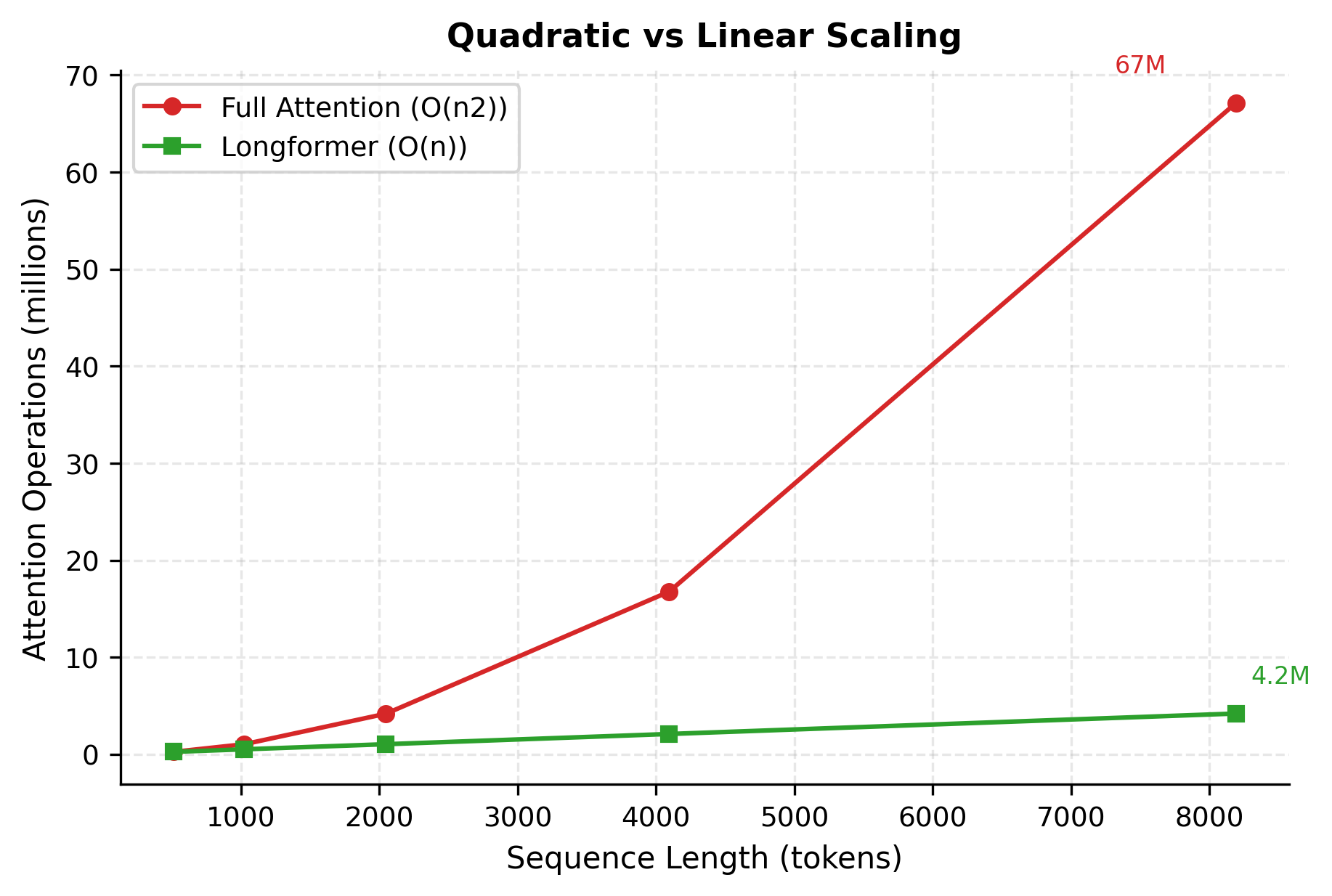
The issue is that this question scales poorly. If you have tokens, each token must compute attention scores, giving us total computations. For a 512-token sequence, that's about 260,000 attention weights per layer. For a 4,096-token document, it explodes to over 16 million. This quadratic scaling is what makes long documents prohibitively expensive.
But here's the key insight: most of these computations are wasted. When you read the word "cat" in a sentence, you don't need to simultaneously consider a word from three paragraphs away to understand its meaning. Most language understanding happens locally. Longformer exploits this observation by restricting which tokens each position can attend to.
Dividing the Sequence: Local and Global Tokens
Longformer partitions the sequence into two distinct sets:
- Local tokens : The vast majority of tokens, which only need to see their immediate neighborhood
- Global tokens : A small number of special tokens that need to aggregate information from the entire sequence
For a sequence of length , we typically have local tokens and global tokens. This asymmetry is the source of Longformer's efficiency: we do expensive full-sequence attention for only a handful of tokens, while the rest use a much cheaper local pattern.
Sliding Window Attention: The Local Pattern
For local tokens, we define a window of size centered on each position. Instead of attending to all tokens, position only attends to positions within the range . Think of it as a spotlight that follows each token, illuminating only its immediate neighborhood.
This restriction is not just a computational trick. It reflects a genuine property of language: most syntactic and semantic relationships are local. Subjects tend to be near their verbs. Adjectives modify nearby nouns. Pronouns typically refer to recently mentioned entities. By focusing attention on a fixed-size window, we capture the dependencies that matter most while ignoring distant positions that rarely contribute meaningful information.
The formal computation for a local token at position is:
Let's unpack each component:
-
: The query vector for position . This is what the token is "asking for" from other positions. We compute it by projecting the input embedding through a learned weight matrix .
-
: The key matrix containing only keys for tokens in the local window. This is a matrix of shape where each row is the key vector for one position in the window. Keys represent what each position "offers" to other tokens.
-
: The value matrix for the same window, also shape . Values contain the actual information that gets aggregated. The attention weights determine how much of each value to include in the output.
-
: The dimension of key and query vectors, typically 64 in base transformer models.
-
: A scaling factor that prevents attention scores from growing too large. Without this, dot products between high-dimensional vectors can become very large, causing softmax to produce nearly one-hot distributions that are hard to learn from.
The computation proceeds through three carefully designed steps:
-
Score computation: We compute , which produces a vector of scores. Each score measures how well the query at position matches each key in the window. Geometrically, this is a dot product: vectors pointing in similar directions produce high scores.
-
Normalization: We divide by to stabilize the magnitude, then apply softmax to convert raw scores into a probability distribution. The weights now sum to 1, telling us what fraction of attention to allocate to each position.
-
Aggregation: We compute a weighted average of the value vectors using these probabilities. Positions with high attention weights contribute more to the output; positions with low weights contribute less.
The critical complexity reduction comes from step 1: instead of computing scores, we compute only scores. Since is a constant (typically 256 or 512), the cost per token is instead of . Across all tokens, the total complexity is , which is linear in sequence length.
Global Attention: Bridging Distant Positions
Sliding window attention solves the efficiency problem, but it creates a new one: how does information travel between distant parts of the sequence? If token 1 can only see tokens 1-256, and token 4000 can only see tokens 3744-4000, how do they ever communicate?
The answer is global tokens. These are special positions that break the local-only rule. A global token attends to every position in the sequence, and every position attends back to it. Think of global tokens as relay stations: information from any part of the sequence can flow through them to reach any other part.
For a global token at position , the attention computation spans the entire sequence:
where:
- : The query vector for the global token, computed using a separate projection matrix
- : The key matrix for all tokens, shape
- : The value matrix for all tokens, shape
Notice the crucial detail: global tokens use different projection matrices (, , ) than local tokens (, , ). Why? Because local and global attention serve fundamentally different purposes.
When a local token computes attention, it's asking: "Which of my neighbors help me understand my immediate context?" When a global token computes attention, it's asking: "What are the most important pieces of information across the entire document?" These are different questions, and the model benefits from learning different representations to answer them.
The separation also matters for the tokens attending to global positions. When a local token attends to a global token, it should receive a representation tailored for aggregation, not one optimized for local context understanding. The separate projection matrices allow this flexibility.
The Symmetry Property
Global attention is bidirectional: global tokens attend to all positions, and all positions attend back to global tokens. This symmetry is essential for information flow.
Consider document classification with a [CLS] token at position 0. The [CLS] token needs to see the entire document to make a classification decision, so it receives global attention. But equally important, every token in the document can "see" the [CLS] token and incorporate that global context into its own representation. This bidirectional flow ensures that even local tokens have access to document-level information, just mediated through the global tokens rather than computed directly.
Combining the Patterns: The Complete Picture
Now we can see how Longformer attention works as a unified system:
-
Most tokens use sliding window attention, computing relevance only within their local neighborhood. This keeps the bulk of computation cheap.
-
A few tokens (typically [CLS], question tokens, or task-specific markers) use global attention, seeing the entire sequence. This maintains the ability to aggregate long-range information.
-
All tokens can attend to global tokens, even if they're outside the local window. This ensures information can flow from any position to any other position through the global intermediaries.
The result is a sparse attention pattern that covers the essential dependencies while skipping the redundant ones. Local relationships are captured directly. Global relationships are captured through designated relay tokens.
Complexity Analysis: Why It Works
Let's verify that this design actually achieves linear complexity. The total attention computation involves three components:
-
Local attention: Each of the tokens computes attention over a window of size . This contributes to the total cost.
-
Global tokens attending to all: Each of the global tokens attends to all positions. This contributes .
-
All tokens attending to global tokens: Each token includes global positions in its attention set. This cost is already absorbed into the local window computation (global tokens simply become part of the attended set).
The total complexity is:
where:
- : the sequence length, the variable that grows with document size
- : the sliding window size, a constant chosen at model design time (typically 512)
- : the number of global tokens, a constant chosen per task (typically 1 to 10)
The key observation is that is a constant. It doesn't grow with sequence length. This means the overall complexity is , linear in sequence length.
Compare this to standard attention's complexity. When you double the sequence length:
- Standard attention: cost quadruples ()
- Longformer attention: cost only doubles ()
This difference is what enables Longformer to process documents of 4,096 tokens or more on hardware that would run out of memory with standard attention at just 512 tokens.
Visualizing the Attention Pattern
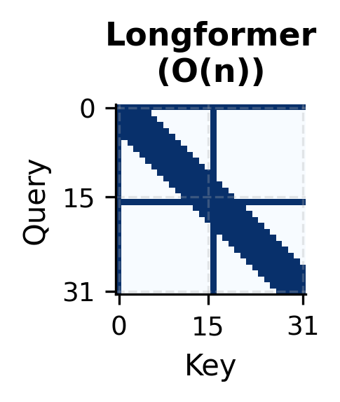
The Longformer attention pattern creates a distinctive sparse structure when visualized as a matrix. Let's build an interactive visualization to understand this pattern.
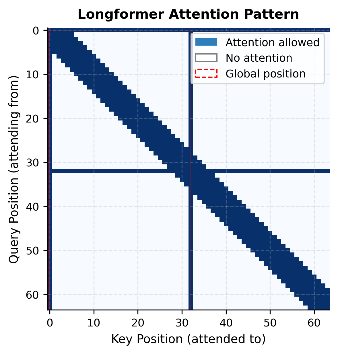
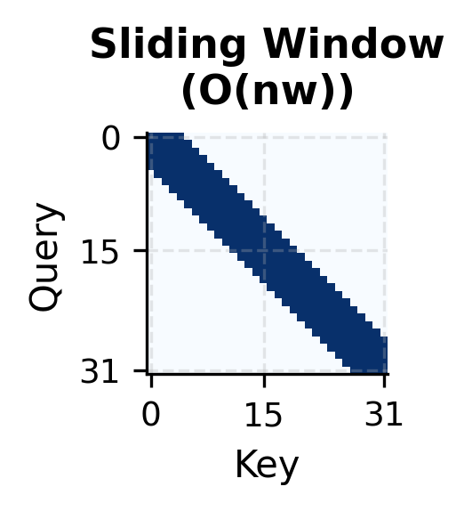
The visualization reveals the structure of Longformer attention. The diagonal band represents sliding window attention: each position attends to its local neighborhood. The vertical and horizontal stripes at positions 0 and 32 show global attention: these tokens have bidirectional access to the entire sequence.
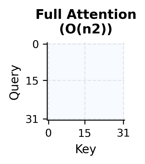
Notice how sparse this pattern is compared to full attention. Full attention would fill the entire square, requiring storage for attention weights (where is our sequence length in this example). The Longformer pattern only needs storage for the non-zero entries, which scales linearly with sequence length.
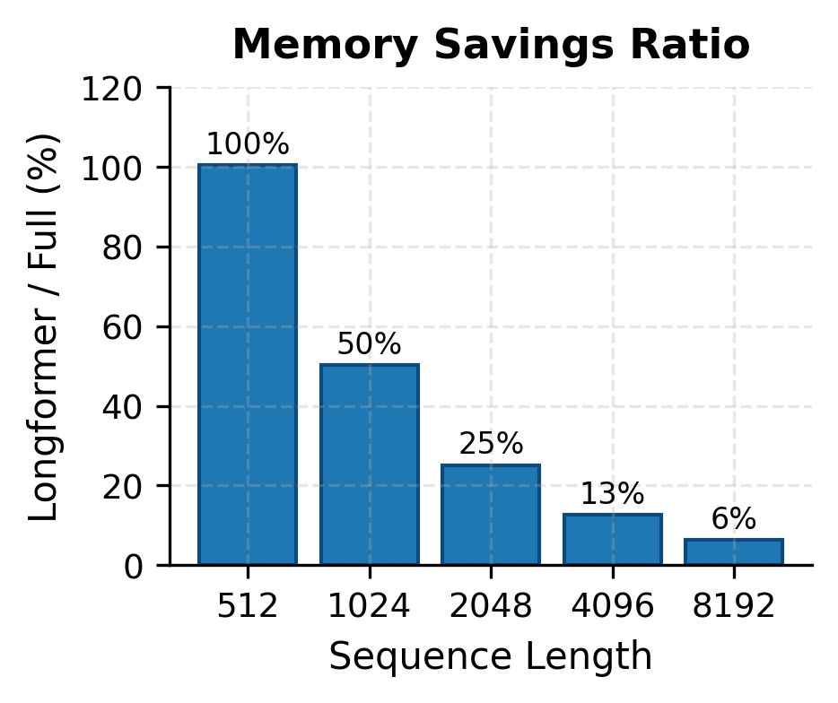
Comparing Attention Sparsity
Let's quantify the sparsity achieved by Longformer compared to full attention.
The numbers tell a compelling story. At 512 tokens, Longformer uses about the same memory as full attention. But as sequence length grows, the savings become dramatic. At 4,096 tokens, Longformer uses only about 12% of the memory. At 16,384 tokens, it drops to around 3%. This is the power of linear versus quadratic scaling.
Implementing Longformer Attention
With the mathematical foundation in place, let's translate these ideas into working code. Building the implementation from scratch solidifies understanding and reveals the practical choices that make Longformer work. We'll start with the simpler sliding window mechanism, then layer on global attention support.
This implementation demonstrates the core sliding window mechanism. Notice how the loop over positions extracts only the local window of keys and values for each query. In production code, this loop would be replaced with efficient sparse matrix operations, but the conceptual structure remains the same: each position computes attention only over its local window, keeping memory usage bounded regardless of sequence length.
The key insight from the code is that the window size half_window determines how far each token can "see." Positions near the edges of the sequence have smaller effective windows (they can't attend to positions that don't exist), but this is handled gracefully by the max and min bounds.
Now let's extend this to the full Longformer attention with global token support:
The implementation reveals several important design decisions:
-
Separate projection matrices: We maintain two complete sets of Q, K, V projections. The local projections (
q_proj,k_proj,v_proj) are used for sliding window attention, while the global projections (q_proj_global,k_proj_global,v_proj_global) are used when global tokens are involved. -
Asymmetric handling: Global tokens use global projections for everything. Local tokens use local projections for local attention, but when attending to global tokens, they use the global key and value vectors. This asymmetry ensures consistent representations regardless of which token is doing the attending.
-
Dynamic attention sets: For local tokens, we compute the union of the local window and global positions. This ensures that even if a global token is outside the local window, every token can still attend to it.
Let's verify our implementation works correctly:
The implementation correctly handles both local sliding window attention and global attention for designated tokens. The output maintains the same shape as the input (batch size 2, sequence length 32, embedding dimension 64), confirming that our attention mechanism preserves dimensionality while routing attention based on the global attention mask. The two global positions (0 and 16) receive full sequence attention, while all other positions use the sliding window of size 8.
Using Longformer from Hugging Face
For practical applications, you'll want to use the optimized Longformer implementation from Hugging Face. Let's see how to apply it to a document classification task.
The document contains over 1,000 tokens, padded to Longformer's maximum sequence length of 4,096. Despite processing this long sequence, only a single token (the [CLS] token at position 0) has global attention. This token's 768-dimensional representation now contains information aggregated from the entire document, enabling downstream tasks like classification or similarity computation without the quadratic memory cost of full attention.
Configuring Global Attention for Different Tasks
The power of Longformer comes from its flexibility in configuring global attention. Different tasks benefit from different global attention patterns.
Document Classification
For classification, you typically only need global attention on the [CLS] token:
Question Answering
For question answering, the question tokens need to see the entire context to find the answer:
The difference in global token count between classification and QA tasks has minimal impact on memory efficiency. Classification uses just 12.5% of full attention memory, while QA with 20 global question tokens uses only 13.5%. Both represent massive savings compared to the 16.7 million attention weights required by full attention at 4,096 tokens.
Named Entity Recognition
For token-level tasks like NER, you might want global attention on sentence boundaries or special delimiter tokens:
The flexibility to configure global attention per task is one of Longformer's key advantages. You control exactly which tokens have global reach, optimizing the trade-off between computational cost and model capability.
Memory and Speed Analysis
Let's measure the actual memory savings achieved by Longformer compared to full attention.
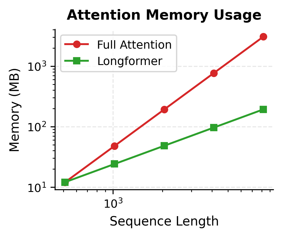
The memory comparison reveals the dramatic difference between full attention and Longformer. At 512 tokens, Longformer uses nearly as much memory as full attention because the window size is comparable to the sequence length. But as sequences grow, the gap widens exponentially. At 8,192 tokens, Longformer uses only about 6% of the memory that full attention would require.
This difference is why Longformer can process 4,096-token documents on hardware that would run out of memory with standard BERT-style attention at just 512 tokens.
Practical Applications
Longformer shines on tasks that require understanding long documents where context from distant parts matters.
Scientific Paper Analysis
Research papers often span 3,000 to 5,000 tokens. A model analyzing citations needs to connect references in the text to the bibliography at the end. The introduction summarizes findings that appear in detail in the results section. Longformer's global attention on section headers and key sentences enables these long-range connections.
Legal Document Review
Contracts frequently cross-reference clauses defined elsewhere in the document. A clause on page 15 might modify conditions stated on page 3. With Longformer, you can designate clause markers as global tokens, allowing the model to track these dependencies across the entire document.
Book Summarization
Summarizing a book chapter requires understanding themes that develop over thousands of words. Characters introduced early affect events that happen much later. Longformer's ability to process long sequences while maintaining global tokens for key narrative elements enables coherent summarization.
Multi-Document Question Answering
When answering questions that require reasoning across multiple documents, you can concatenate them and use global attention on the question tokens. The model can then search across all provided evidence to find the answer.
Limitations and Trade-offs
Longformer represents a significant advance for long document processing, but it comes with trade-offs you should understand before adopting it.
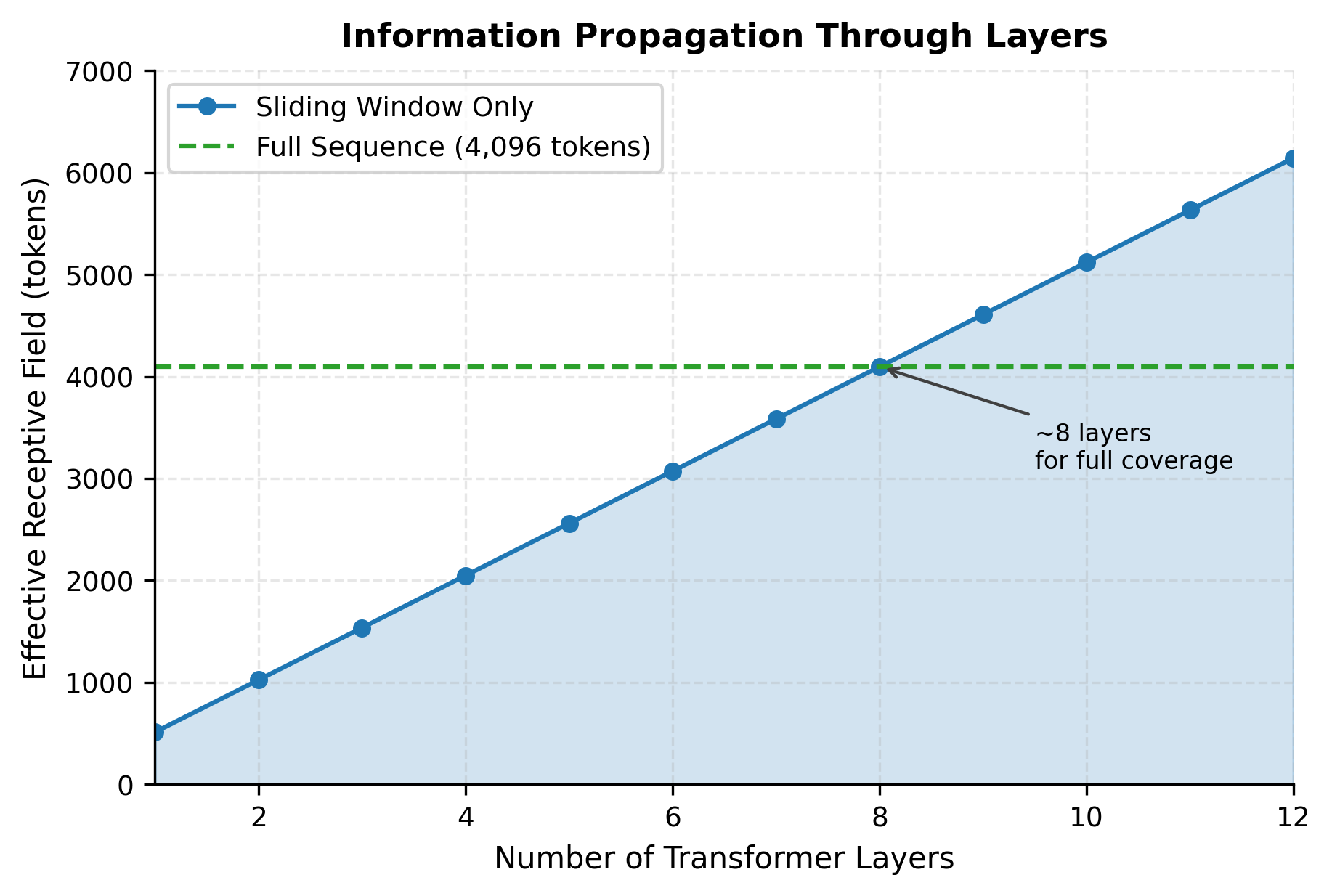
The sliding window creates an information bottleneck for tokens far from any global token. If important information lies 1,000 positions away from the nearest global token and outside any token's window, the model must rely on the stacking of attention layers to propagate that information. Deep transformer stacks help mitigate this through repeated local interactions that gradually spread information, but the effective receptive field is still limited compared to full attention. For tasks where any token might need to attend to any other token equally, Longformer's sparse pattern might lose important connections.
The separate projection matrices for global attention increase parameter count by approximately 50% for the attention layers. For models with billions of parameters, this overhead is significant. You're trading memory during inference for additional model weights that must be stored and loaded. The global projections also add complexity to fine-tuning: you need to carefully initialize them, and learning dynamics can differ between local and global components.
Choosing which tokens should have global attention requires task-specific knowledge. For classification, the [CLS] token is an obvious choice. For question answering, the question tokens work well. But for open-ended tasks like summarization or dialogue, the optimal global attention configuration is less clear. Getting this wrong can significantly hurt performance, and finding the right configuration often requires experimentation.
Finally, Longformer's linear complexity assumes the window size and number of global tokens remain constant as sequence length grows. If your task requires global attention on a growing fraction of tokens (say, one global token per paragraph), complexity can approach again. The linear scaling benefit only materializes when global attention is genuinely sparse.
Key Parameters
When working with Longformer, the following parameters have the greatest impact on model behavior and performance:
-
window_size: Controls how many neighboring tokens each position can attend to. Larger windows capture more context but increase memory usage linearly. The default of 512 works well for most document tasks, but you might reduce it to 256 for memory-constrained environments or increase it for tasks requiring broader local context.
-
global_attention_mask: A binary tensor indicating which tokens have global attention. Set to 1 for tokens that need to see the entire sequence (e.g., [CLS] for classification, question tokens for QA). Keep the number of global tokens small to maintain linear complexity.
-
max_length: Maximum sequence length the model can process. Longformer-base supports 4,096 tokens by default. Longer sequences require more memory and compute, but the linear scaling makes lengths up to 16,384 feasible.
-
attention_mode (in custom implementations): Determines whether to use sliding window only, global only, or the hybrid pattern. The hybrid pattern is standard for most tasks.
When fine-tuning Longformer, pay special attention to the global attention configuration. The pretrained model learns both local and global projection matrices, so changing which tokens receive global attention during fine-tuning is straightforward. However, adding too many global tokens can negate the efficiency benefits that make Longformer attractive for long documents.
Summary
Longformer tackles the quadratic attention bottleneck through an elegant combination of local and global attention patterns. The key ideas are:
-
Sliding window attention reduces per-token complexity from to , where is the window size. Most tokens only need local context to understand their meaning.
-
Global attention preserves the ability to aggregate information across the entire sequence. By designating specific tokens as global, you maintain long-range dependencies where they matter most.
-
Separate projections for local and global attention allow the model to learn distinct representations for different types of context aggregation.
-
Linear complexity enables processing sequences of 4,096 tokens or more on hardware that would fail with standard attention at 512 tokens.
The practical impact is substantial. Research papers, legal documents, and book chapters that were previously too long for transformer processing are now accessible. Tasks requiring reasoning across thousands of tokens become feasible without the memory explosion of full attention.
Longformer represents a broader trend in efficient attention: recognizing that the dense attention pattern of standard transformers is often more than necessary. By designing sparse patterns that match the actual information flow needed for a task, we can dramatically reduce computational costs while maintaining model quality.
Quiz
Ready to test your understanding? Take this quick quiz to reinforce what you've learned about Longformer's efficient attention mechanism.

Comments