

Learn how Position Interpolation extends transformer context windows by scaling position indices to stay within training distributions, enabling longer sequences with minimal fine-tuning.

This article is part of the free-to-read Language AI Handbook
Choose your expertise level to adjust how many terms are explained. Beginners see more tooltips, experts see fewer to maintain reading flow. Hover over underlined terms for instant definitions.
Position Interpolation
Modern language models face a fundamental tension: training on long sequences is expensive, but real-world applications demand them. A model trained on 2,048 tokens might encounter documents with 8,000 tokens, conversations spanning 16,000 tokens, or codebases requiring even longer context. When RoPE-based models try to process positions beyond their training range, performance degrades rapidly. The rotation angles reach values the model has never seen, producing attention patterns that bear no resemblance to what was learned.
Position Interpolation, introduced by Chen et al. in 2023, offers an elegant solution: instead of extrapolating to unseen positions, we interpolate within the familiar range. Rather than assigning position 4,096 a rotation angle the model has never encountered, we scale all positions down so they fit within the original training range. Position 4,096 becomes position 2,048 after scaling, and the model sees familiar rotation angles even as it processes longer sequences.
This chapter develops Position Interpolation from first principles. We'll start by understanding why RoPE fails at extrapolation, derive the interpolation formula, implement it in code, and explore its limitations. By the end, you'll understand both the elegance of this approach and why subsequent methods like NTK-aware scaling were developed to address its shortcomings.
The Extrapolation Problem
RoPE encodes position through rotation. At position , each dimension pair of the query and key vectors is rotated by an angle proportional to . The key idea is that each dimension pair rotates at a different frequency, creating a unique positional signature. The rotation angle for dimension pair at position is computed as:
where:
- : the rotation angle (in radians) applied to dimension pair at sequence position
- : the position index in the sequence (0, 1, 2, ..., for a sequence of length )
- : the dimension pair index (0, 1, 2, ..., )
- : the total embedding dimension (typically 64, 128, or larger)
- : a constant that controls the range of frequencies (typically 10000)
- : the base frequency for dimension pair , which decreases exponentially as increases
The exponential decay in the base frequency means that dimension pair 0 rotates fastest (with radian per position), while higher-indexed pairs rotate progressively slower. This creates a multi-scale representation where different dimension pairs capture positional information at different granularities.
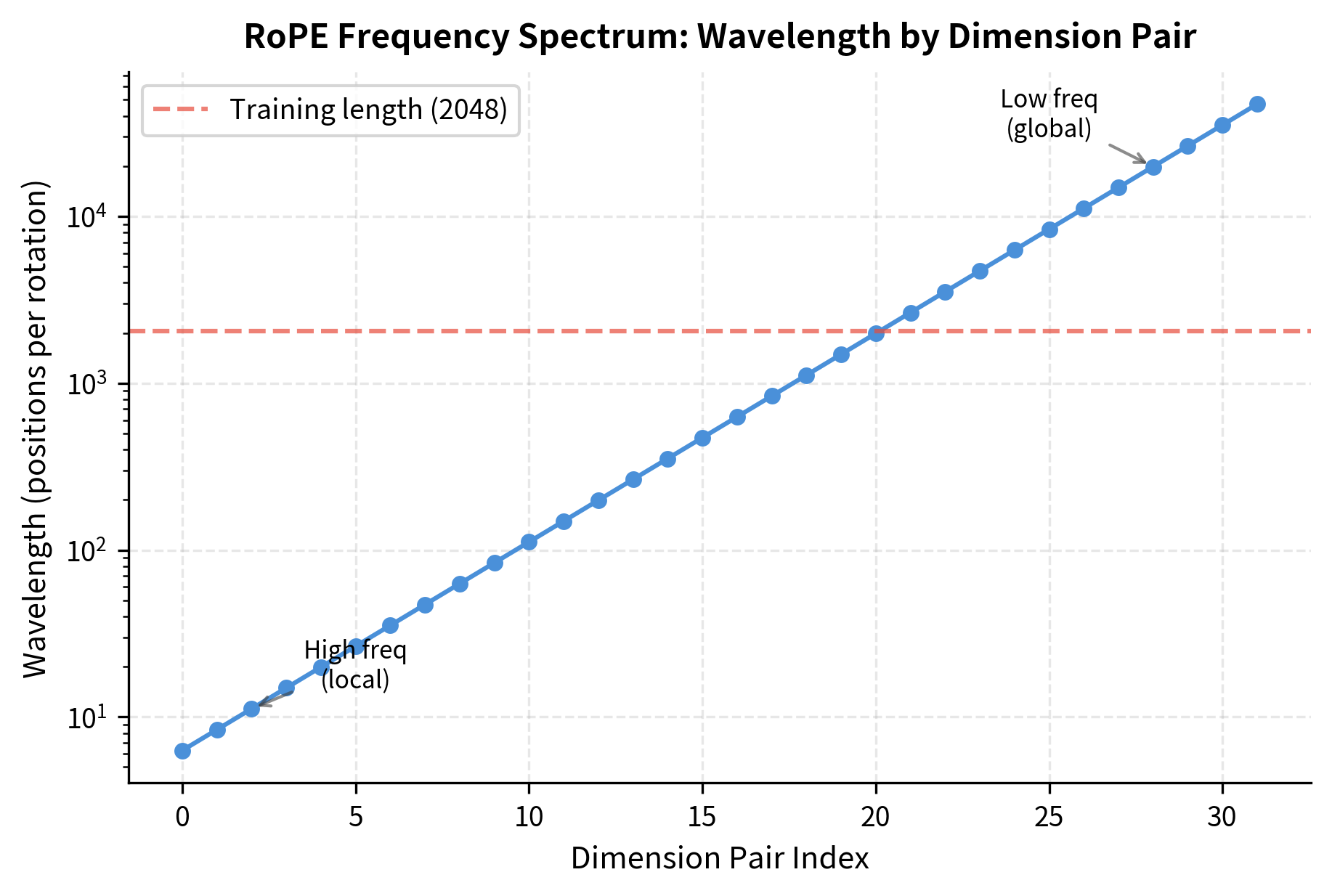
During training on sequences of length , the model sees positions . The rotation angles range from 0 to for each dimension pair.
What happens when we present the model with position ? The rotation angle exceeds anything seen during training. For the fastest-rotating dimensions (where is large), these new angles produce embedding rotations the attention mechanism has never learned to interpret.
Let's visualize this problem by examining the rotation angles at different positions.
For the fastest-rotating dimension pair (pair 0), the model sees angles up to about 2,047 radians during training. Extending to 4x the context pushes this to over 8,000 radians. While both values wrap around the unit circle many times, the relative patterns between dimension pairs change in ways the model hasn't learned.
The real problem becomes clear when we examine what happens to attention patterns. During training, the model learns that certain rotation angle combinations correspond to meaningful relative positions. When extrapolated angles produce unfamiliar combinations, the learned attention patterns break down.
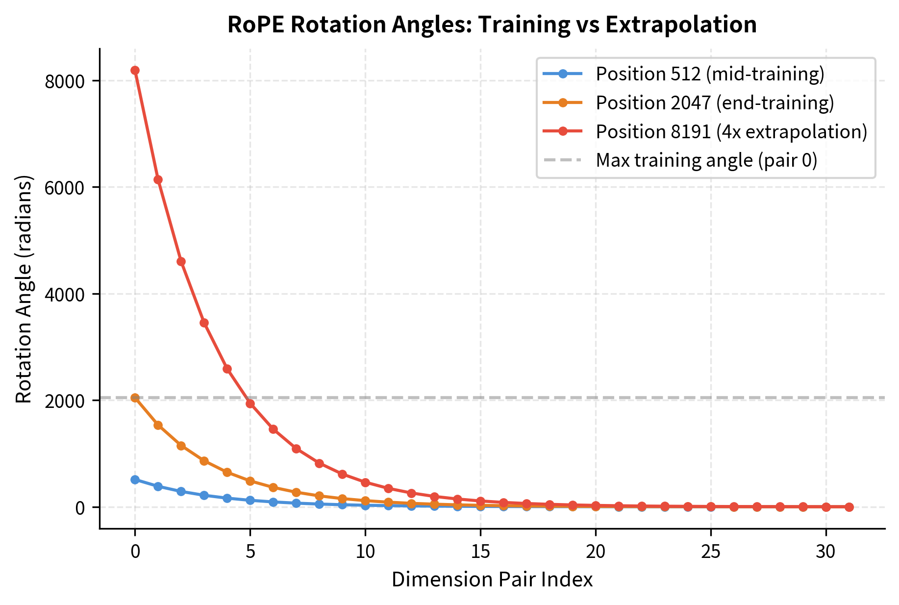
The plot reveals the core issue. Fast-rotating dimensions (low indices) experience dramatic angle increases during extrapolation. The angle at position 8191 for dimension pair 0 is four times larger than at position 2047. Meanwhile, slow-rotating dimensions (high indices) barely change. This asymmetric behavior disrupts the carefully balanced patterns the model learned during training.
The Interpolation Insight
We've seen that extrapolation fails because the model encounters rotation angles outside its training distribution. But what if we could ensure that every position, no matter how far into the extended sequence, produces angles the model has already seen? This is the core intuition behind Position Interpolation.
From Intuition to Formulation
Think of the training range as a ruler. During training, the model learned to interpret positions from 0 to , each marking a specific location on this ruler. Now we need to fit a longer sequence onto the same ruler. The solution? We don't extend the ruler; we compress the new positions to fit within the existing marks.
If we want to process a sequence of length where , we define a scale factor that maps the extended range back to the familiar one:
where:
- : the scale factor, always between 0 and 1 when extending context
- : the maximum sequence length seen during training (e.g., 2048)
- : the target extended sequence length (e.g., 8192)
This scale factor answers the question: "How much do we need to shrink the extended positions to fit them within the training range?" For a 4x extension (2K to 8K), , meaning every position is compressed to one-quarter of its original value.
Position Mapping in Action
Let's trace through concrete examples to see how this mapping works. For a model trained on 2,048 positions processing an 8,192-token sequence:
| Actual Position | Scaled Position () | Interpretation |
|---|---|---|
| 0 | 0 | Start of sequence, unchanged |
| 2,048 | 512 | Maps to quarter of training range |
| 4,096 | 1,024 | Maps to midpoint of training range |
| 8,191 | 2,047.75 | Maps to end of training range |
Every position in the extended sequence, no matter how large, maps to a value the model encountered during training. Position 8,191 in the extended sequence produces the same rotation pattern as position 2,047 would in the original system.
Position Interpolation scales position indices by a factor before computing RoPE rotation angles. This keeps all rotation angles within the range seen during training, trading extrapolation for interpolation.
Deriving the Modified RoPE Formula
Now we can formalize this intuition mathematically. The derivation proceeds in three steps, each building naturally on the previous.
Step 1: Recall the original RoPE rotation angle.
In standard RoPE, the rotation angle for dimension pair at position is simply the product of position and base frequency:
where is the base frequency for dimension pair . This formula produces angles that grow linearly with position, which is exactly the behavior that causes extrapolation to fail when exceeds the training range.
Step 2: Apply position scaling to compress the range.
Position Interpolation modifies this formula by scaling the position index before computing the rotation. Instead of using directly, we use :
We can rearrange this expression to reveal an important insight:
where:
- : the position-interpolated rotation angle for dimension pair at position
- : the actual position in the extended sequence
- : the scale factor ()
- : the original base frequency for dimension pair
The rearrangement shows two equivalent interpretations of Position Interpolation:
- Scale the position: Compute angles for position using original frequencies
- Scale the frequency: Compute angles for position using reduced frequencies
Both perspectives lead to the same result, but the second interpretation proves useful for implementation.
Step 3: Express as modified base frequency.
Let's push the algebraic manipulation further to see what Position Interpolation does to the effective RoPE base:
We can factor out the scale to express this in terms of a modified base:
This reveals that Position Interpolation is mathematically equivalent to using a larger effective base:
For extending from 2K to 8K context (), the effective base becomes . Why does a larger base help? Recall that the base frequency is . A larger base produces smaller frequencies, which means slower rotations for all dimension pairs. Slower rotations let us fit more positions into the same angular range before exceeding the training maximum.
Connecting Math to Mechanism
The mathematical derivation reveals something elegant: Position Interpolation doesn't change the fundamental structure of RoPE. It doesn't add new components or modify the attention mechanism. It simply asks: "What if we used a different base constant from the start?" The answer is that a larger base would have allowed longer sequences all along, but at the cost of reduced angular resolution between nearby positions.
This insight also explains why fine-tuning is necessary. The model learned to associate certain rotation patterns with certain relative distances. When we compress positions, those associations break. A distance of 100 positions now produces the same rotation pattern as 25 positions would have during training. Fine-tuning recalibrates these associations.
Implementing Position Interpolation
With the mathematical foundation in place, let's translate Position Interpolation into code. The implementation is remarkably simple: we compute the scale factor, multiply positions by that factor, and then proceed with standard RoPE angle computation.
Computing Interpolated Angles
The core function takes positions along with both the training and target lengths. It computes the scale factor internally, scales all positions, and returns angles that stay within the training range.
Verifying the Angle Bounds
The critical test: do the interpolated angles at the maximum extended position match the training maximum? Let's compare the angles at position 8191 across three methods.
The results confirm our mathematical derivation. With Position Interpolation, the maximum angles at position 8191 match the training maximum at position 2047 across all dimension pairs. Original RoPE would produce angles 4x larger at the extended position, but Position Interpolation compresses them back into the familiar range.
Let's visualize this comparison as a heatmap to see the pattern across all dimension pairs simultaneously.
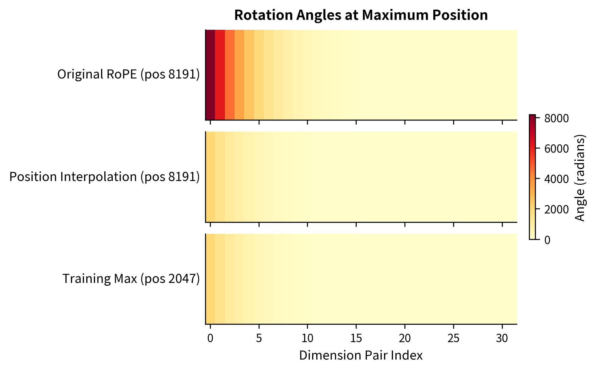
The heatmap makes the difference visually striking. The top row shows the intense "heat" of original RoPE's extrapolated angles, especially in the fast-rotating dimensions on the left. Position Interpolation (middle row) shows the same pattern as the training maximum (bottom row), confirming that we've successfully mapped extended positions back into familiar territory.
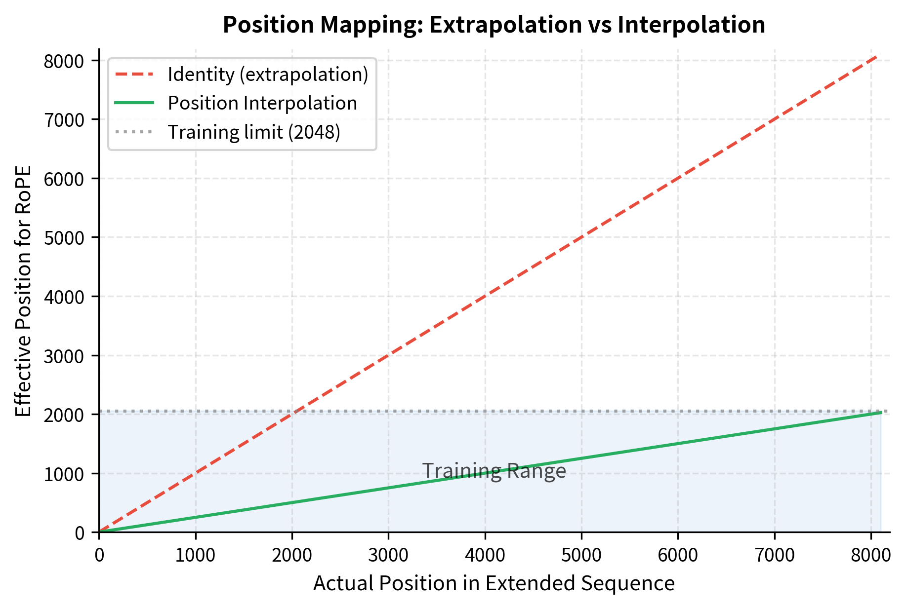
Visualizing the Position Mapping
Let's visualize this compression graphically. The plot below shows how actual positions in the extended sequence map to effective positions for RoPE computation.
Interpolation vs Extrapolation: A Closer Look
Why does interpolation work better than extrapolation? The answer lies in how neural networks generalize. During training, the model learns attention patterns for rotation angles in a specific range. These learned patterns form a continuous function over that range.
When we extrapolate, we ask the model to generalize this function to inputs it has never seen. Neural networks are notoriously poor at extrapolation; they often produce arbitrary outputs outside their training distribution. When we interpolate, we stay within the training distribution but query it at finer-grained positions. The model can leverage its learned continuous representations to handle intermediate values.
Consider an analogy. Imagine training someone to recognize temperatures between 0°C and 100°C. If you then ask them about 200°C, they must extrapolate beyond their experience, and their predictions become unreliable. But if you ask about 37.5°C when they've only seen integer values, they can interpolate from their knowledge of 37°C and 38°C.
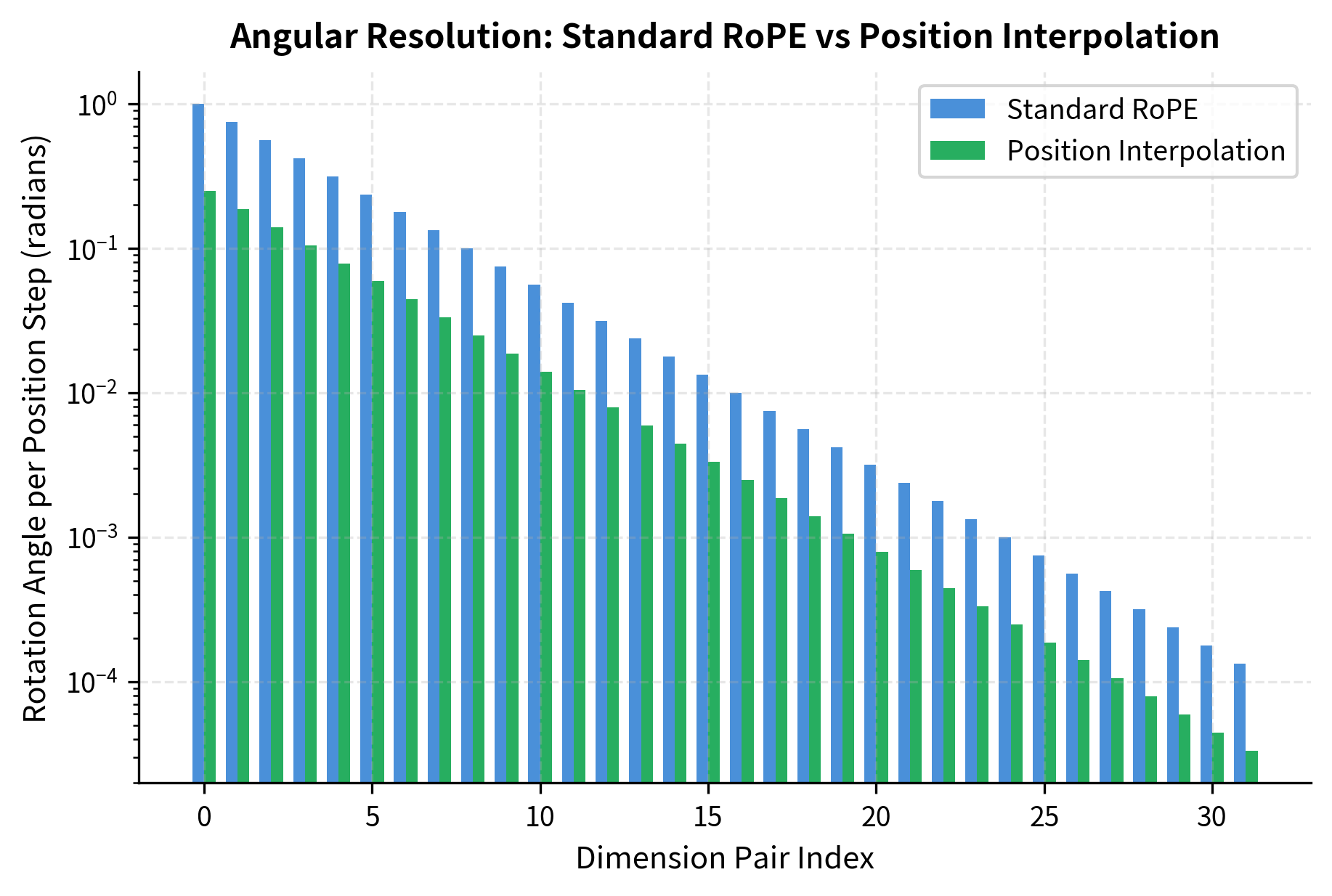
Let's quantify this by examining how the angle differences (which determine attention scores) change under interpolation.
The relative angle per position step shrinks with interpolation. In standard RoPE, moving one position rotates dimension pair 0 by 1 radian. With 4x interpolation, the same step rotates by only 0.25 radians. This compression is the trade-off at the heart of Position Interpolation: we maintain familiar absolute angles but reduce the angular resolution between nearby positions.
Fine-tuning for Extended Context
Position Interpolation alone doesn't magically enable long context. While the rotation angles stay within the training distribution, the model still encounters unfamiliar situations. Two tokens that were 100 positions apart during training now produce the same relative rotation as tokens 400 positions apart in the extended sequence. The model must learn to interpret these compressed position signals.
This is where fine-tuning comes in. After applying Position Interpolation, models typically undergo a short fine-tuning phase on long-context data. The good news: this fine-tuning is remarkably efficient. Chen et al. found that only about 1,000 fine-tuning steps were needed to adapt a 2K-context LLaMA model to 8K context, compared to the billions of tokens used in original pretraining.
Position Interpolation requires fine-tuning to achieve good performance. Without fine-tuning, the model may produce coherent outputs at the new context length, but perplexity typically increases. The fine-tuning phase teaches the model to interpret the compressed position signals correctly.
Let's simulate what fine-tuning might need to correct by examining how attention patterns change under interpolation.
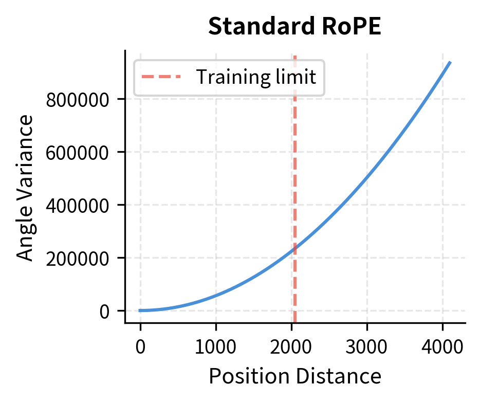
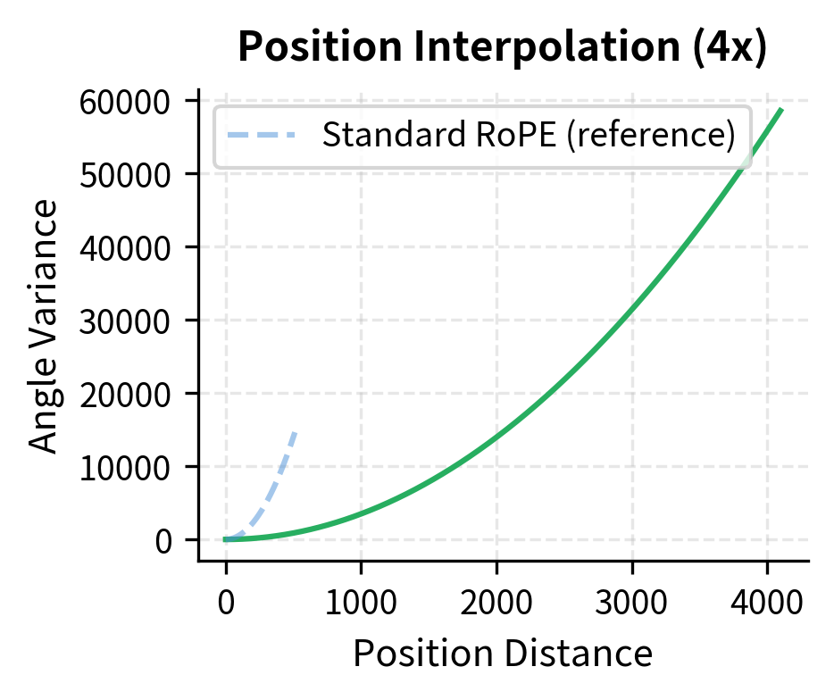
The plots illustrate the core transformation. With Position Interpolation, a distance of 4,096 positions produces the same rotation angle pattern as a distance of 1,024 positions in standard RoPE. Fine-tuning teaches the model that this compressed pattern now represents the longer distance.
A Complete Implementation
Let's put everything together into a complete Position Interpolation implementation that can be applied to RoPE.
Let's verify that our implementation produces the expected behavior.
The interpolated rotation matrix at position 6,000 matches the standard rotation matrix at position 1,500, confirming that our implementation correctly maps extended positions back to the training range.
Limitations of Position Interpolation
Position Interpolation enables longer context, but it comes with trade-offs. Understanding these limitations helps explain why subsequent methods like NTK-aware scaling were developed.
Reduced positional resolution. The most significant limitation is reduced angular resolution between nearby positions. When we compress 8,192 positions into the range of 2,048, each position step produces 1/4 the rotation of the original. Two tokens that are adjacent in the extended sequence differ by the same rotation as tokens 0.25 positions apart in the original. This compression can make it harder for the model to distinguish nearby positions, potentially affecting tasks requiring fine-grained positional awareness.
Non-uniform frequency scaling. Position Interpolation applies the same scale factor to all frequency components. However, different frequencies may require different treatment. High-frequency components (fast-rotating dimensions) are most affected by the reduced resolution because they distinguish local positions. Low-frequency components (slow-rotating dimensions) were already coarse and are less impacted. This uniform scaling is suboptimal, which motivated the development of NTK-aware scaling that treats frequencies differently.
Fine-tuning requirement. While Position Interpolation requires far less fine-tuning than training from scratch, it still requires some adaptation. This limits scenarios where you need to extend context on the fly without access to fine-tuning data or compute.
Perplexity increase. Even after fine-tuning, models with Position Interpolation often show slightly higher perplexity compared to models trained directly on longer sequences. The compression introduces information loss that fine-tuning can mitigate but not fully eliminate.
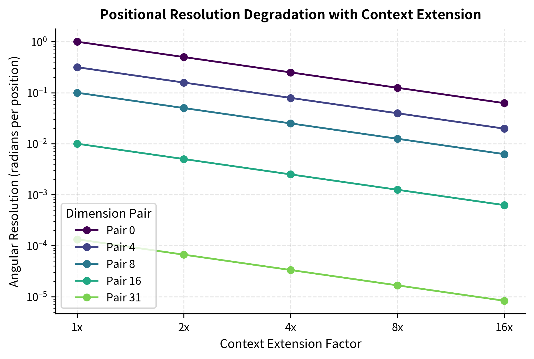
Let's quantify how different dimension pairs are affected by the uniform scaling.
The analysis reveals the asymmetric impact. High-frequency dimension pairs, which originally completed a rotation every 6-50 positions, now require 4x as many positions. This affects local position discrimination most severely. Low-frequency dimension pairs, already operating at wavelengths of thousands of positions, remain capable of distinguishing positions at the extended range.
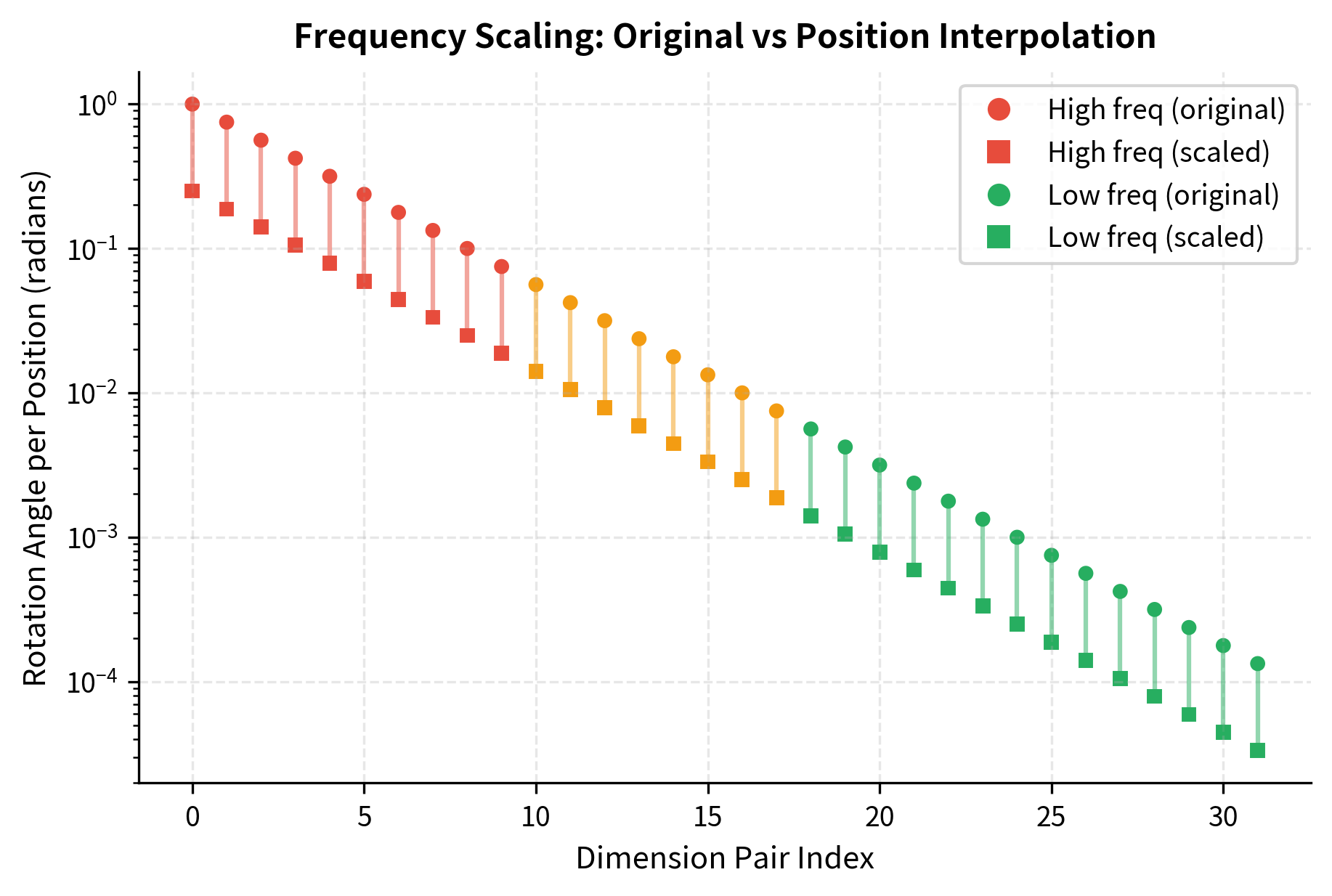
The visualization shows how Position Interpolation uniformly scales all frequencies by the same factor (4x reduction). The vertical lines connecting original (circles) to scaled (squares) values have the same proportional length across all dimension pairs. This uniform treatment is the core limitation that NTK-aware scaling addresses.
Key Parameters
When implementing Position Interpolation, the following parameters control the behavior:
-
train_length: The maximum sequence length the model was originally trained on (e.g., 2048 for LLaMA). This defines the upper bound of positions the model has learned to interpret during pretraining. -
target_length: The extended context length you want to support (e.g., 8192). Must be greater thantrain_lengthfor interpolation to apply. -
scale: Computed astrain_length / target_length. This determines how much to compress positions. A scale of 0.25 means 4x context extension. Smaller scale values enable longer contexts but reduce positional resolution proportionally. -
base: The RoPE base constant (typically 10000). Position Interpolation effectively increases this tobase / scale, slowing all rotations uniformly. -
d_model: The embedding dimension. Must be even since RoPE operates on dimension pairs. Each pair rotates at a different frequency determined by its index.
When selecting parameters, consider the trade-off between context length and positional resolution. Extending by 2x is generally safe with minimal fine-tuning. Extensions of 4x-8x work well but require more fine-tuning to recover performance. Extensions beyond 8x may significantly degrade the model's ability to distinguish nearby positions.
Summary
Position Interpolation provides an elegant solution to the context length extension problem. By scaling position indices rather than extrapolating to unseen values, it keeps all rotation angles within the training distribution. The key insights include:
-
Interpolation over extrapolation. Neural networks generalize poorly outside their training distribution. By scaling positions down instead of letting them grow, Position Interpolation stays within familiar territory.
-
Simple implementation. The technique requires only a scale factor applied to position indices before computing RoPE. No architectural changes are needed.
-
Efficient fine-tuning. Adapting a model to extended context requires only about 1,000 fine-tuning steps, orders of magnitude less than original pretraining.
-
Uniform scaling limitation. All frequency components receive the same scaling treatment, which is suboptimal. High-frequency dimensions, crucial for local position discrimination, lose the most resolution.
The limitations of Position Interpolation, particularly its uniform treatment of frequencies, motivated the development of NTK-aware scaling, which we'll explore in the next chapter. That technique applies frequency-dependent scaling, preserving high-frequency components while adjusting low-frequency ones, achieving better performance without sacrificing local positional awareness.
Quiz
Ready to test your understanding? Take this quick quiz to reinforce what you've learned about Position Interpolation and extending context length in language models.

Comments