Search

Search articles

FlashAttention Implementation: GPU Memory Optimization for Transformers

Michael BrenndoerferUpdated June 30, 202553 min read

Master FlashAttention's tiled computation and online softmax algorithms. Learn GPU memory hierarchy, CUDA kernel basics, and practical PyTorch integration.

Track your reading progress

Sign in to mark chapters as read and track your learning journey

Sign in →
Reading Level

Choose your expertise level to adjust how many terms are explained. Beginners see more tooltips, experts see fewer to maintain reading flow. Hover over underlined terms for instant definitions.

FlashAttention Implementation

FlashAttention changes how we think about attention computation. Rather than viewing the attention formula as a mathematical specification to implement directly, FlashAttention treats it as a memory optimization problem. The algorithm produces identical outputs to standard attention but restructures the computation to minimize memory transfers between GPU memory hierarchies. Understanding how FlashAttention achieves this requires diving into GPU architecture, memory access patterns, and the algorithmic techniques that make it all work.

This chapter explores the implementation details of FlashAttention, from the fundamentals of GPU memory to practical usage in PyTorch. We'll examine CUDA kernel basics, understand why memory access patterns matter so much for performance, trace the improvements from FlashAttention to FlashAttention-2, and see how to use these techniques in your own models. By the end, you'll understand both the theoretical foundations and practical applications of what has become the de facto standard for attention computation in modern LLMs.

GPU Memory Hierarchy

Before understanding FlashAttention, you need to understand where bottlenecks actually occur on GPUs. Modern deep learning is often described as "compute-bound," but attention computation is actually "memory-bound." This distinction is crucial.

Memory-Bound vs Compute-Bound

A computation is compute-bound when the limiting factor is the number of arithmetic operations the processor can perform. A computation is memory-bound when the limiting factor is how quickly data can be transferred to and from memory. Attention is memory-bound because we spend more time moving data than computing with it.

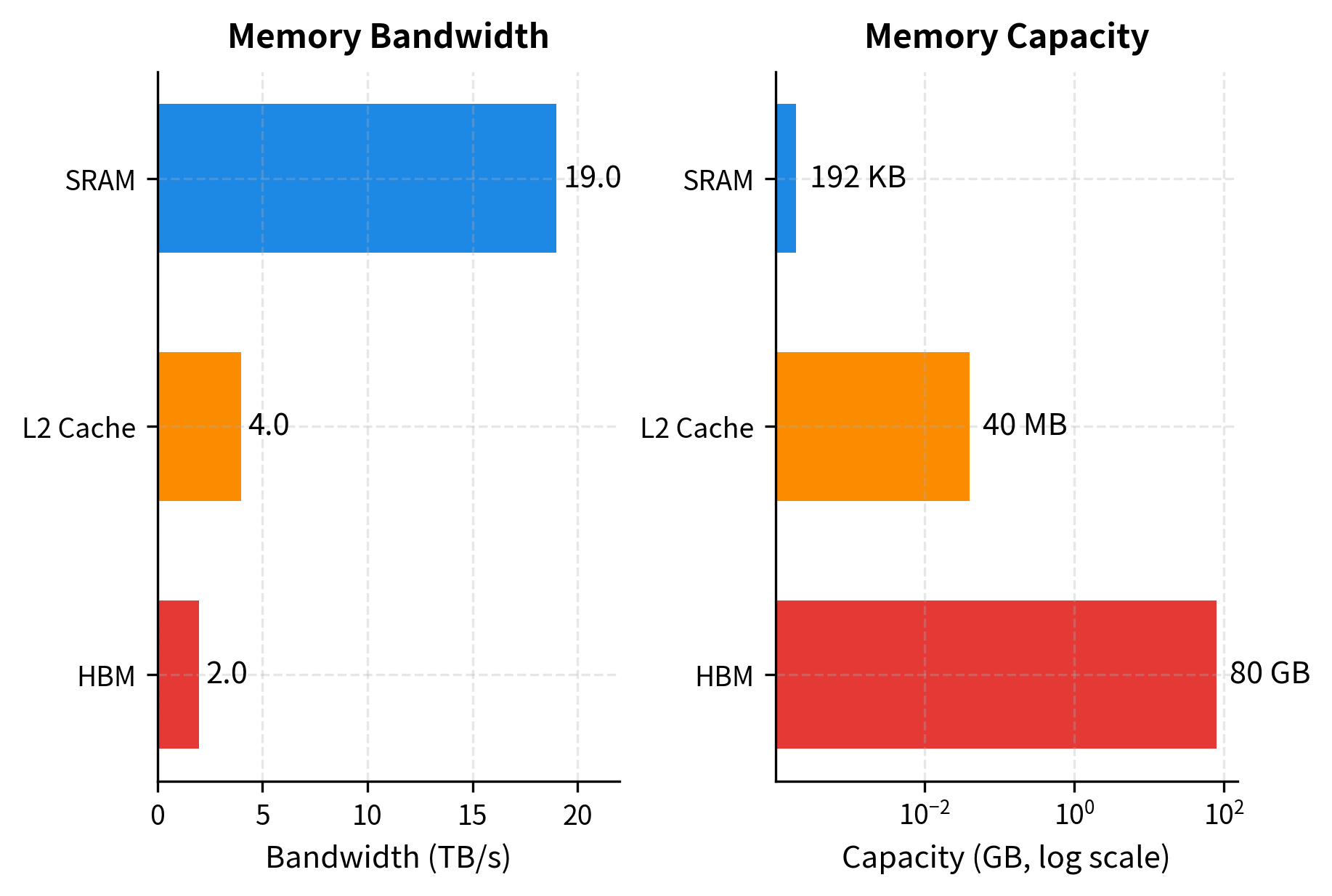
GPUs have a hierarchical memory structure with three main levels, each with different speeds and capacities:

In[2]:
Code
def gpu_memory_specs():
    """
    Approximate specifications for NVIDIA A100 GPU memory hierarchy.
    These numbers illustrate the dramatic differences between memory levels.
    """
    specs = {
        "HBM (High Bandwidth Memory)": {
            "capacity_gb": 80,
            "bandwidth_tb_s": 2.0,
            "latency_ns": 200,
        },
        "L2 Cache": {
            "capacity_gb": 0.040,  # 40 MB
            "bandwidth_tb_s": 4.0,
            "latency_ns": 50,
        },
        "SRAM (Registers + Shared Memory)": {
            "capacity_gb": 0.000192,  # 192 KB per SM, ~108 SMs
            "bandwidth_tb_s": 19.0,
            "latency_ns": 5,
        },
    }
    return specs


specs = gpu_memory_specs()
Out[3]:
Console
NVIDIA A100 GPU Memory Hierarchy:

Level                                        Capacity       Bandwidth      Latency
----------------------------------------------------------------------------------
HBM (High Bandwidth Memory)                     80 GB        2.0 TB/s       200 ns
L2 Cache                                      40.0 MB        4.0 TB/s        50 ns
SRAM (Registers + Shared Memory)               0.2 MB       19.0 TB/s         5 ns

The numbers reveal a fundamental tension. HBM (the main GPU memory where tensors live) has enormous capacity but relatively slow access. SRAM (registers and shared memory) is much faster but tiny. The speed difference is nearly 10x, while the capacity difference is over 400,000x. Standard attention computation repeatedly reads and writes to HBM, suffering the slow access speeds. FlashAttention restructures the computation to keep data in SRAM as long as possible.

Out[4]:
Visualization
Bar chart comparing GPU memory levels by bandwidth and capacity, showing SRAM with highest bandwidth but smallest capacity.
GPU memory hierarchy showing the trade-off between capacity and bandwidth. FlashAttention exploits this hierarchy by computing attention in small blocks that fit in SRAM, avoiding repeated HBM transfers.

Why Standard Attention is Memory-Bound

Consider what happens during standard attention computation:

  1. Load Q, K, V from HBM to compute S=QKTS = QK^T
  2. Write S back to HBM (this is an n×nn \times n matrix)
  3. Load S from HBM to compute softmax
  4. Write attention weights P back to HBM
  5. Load P and V from HBM to compute output
  6. Write output back to HBM

Each step involves transfers to and from the slow HBM. The n×nn \times n matrices S and P are particularly problematic: for a sequence of 4096 tokens with 32-bit floats, each matrix is 64 MB. With 32 attention heads, that's 2 GB just for intermediate storage, per layer, per batch element.

In[5]:
Code
def memory_transfers_standard_attention(n, d, dtype_bytes=4):
    """
    Calculate memory transferred in standard attention.

    Args:
        n: Sequence length
        d: Model dimension
        dtype_bytes: Bytes per element (4 for fp32, 2 for fp16)

    Returns:
        Dictionary with memory transfer statistics
    """
    # Input matrices Q, K, V: each n x d
    input_read = 3 * n * d * dtype_bytes

    # Score matrix S = QK^T: n x n, written then read for softmax
    score_write = n * n * dtype_bytes
    score_read = n * n * dtype_bytes

    # Attention weights P after softmax: n x n, written then read
    weights_write = n * n * dtype_bytes
    weights_read = n * n * dtype_bytes

    # V read again for P @ V
    v_read = n * d * dtype_bytes

    # Output: n x d
    output_write = n * d * dtype_bytes

    total = (
        input_read
        + score_write
        + score_read
        + weights_write
        + weights_read
        + v_read
        + output_write
    )

    return {
        "input_read_mb": input_read / 1e6,
        "intermediate_mb": (
            score_write + score_read + weights_write + weights_read
        )
        / 1e6,
        "output_mb": output_write / 1e6,
        "total_mb": total / 1e6,
    }


# Example: typical transformer settings
transfers = memory_transfers_standard_attention(n=4096, d=768, dtype_bytes=4)
Out[6]:
Console
Memory Transfers in Standard Attention (n=4096, d=768, fp32):

  Input Q, K, V:         37.7 MB
  Intermediate S, P:    268.4 MB
  Output:                12.6 MB
  Total transfers:      331.4 MB

The n×n intermediate matrices dominate memory traffic.

The intermediate matrices consume over 128 MB of memory transfers, dwarfing the input and output. This is where FlashAttention intervenes: by never materializing the full n×nn \times n matrices, it eliminates most of this memory traffic.

CUDA Kernel Basics

FlashAttention is implemented as a custom CUDA kernel, meaning it runs directly on GPU hardware with fine-grained control over memory access. Understanding a few CUDA concepts helps appreciate what FlashAttention does under the hood.

CUDA Kernel

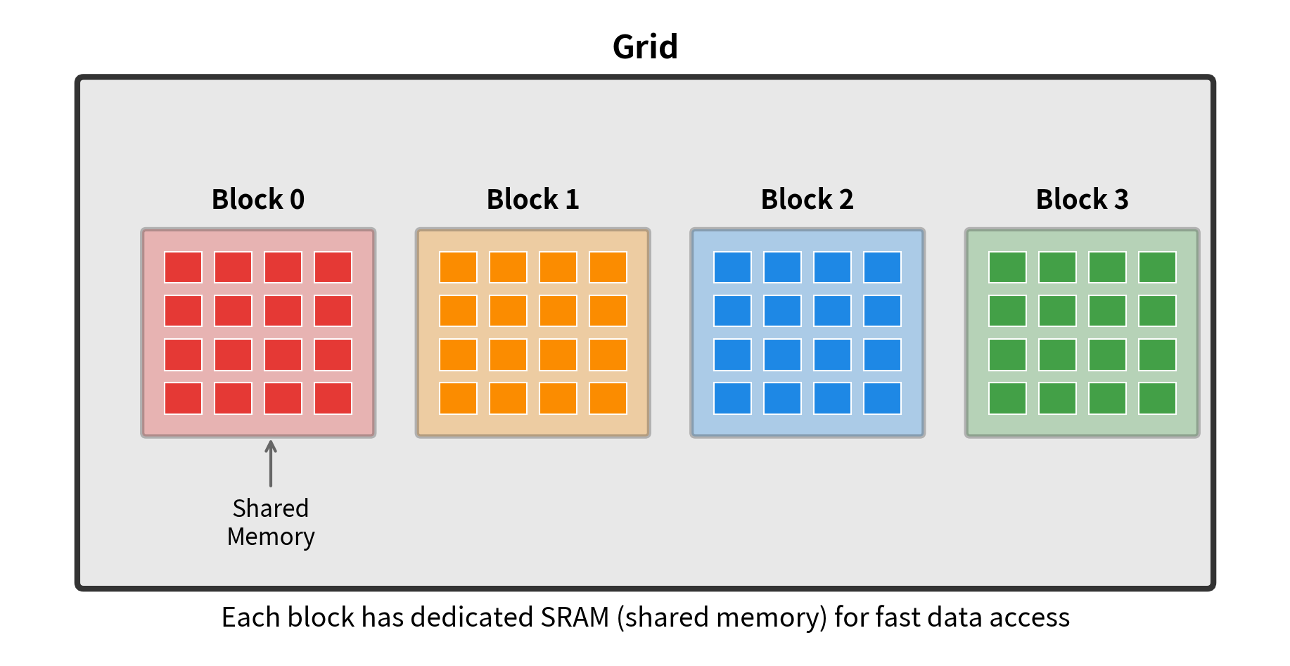
A CUDA kernel is a function that runs on the GPU across many parallel threads. Threads are organized into blocks, and blocks are organized into a grid. Each thread can access different levels of memory: registers (private to the thread), shared memory (shared within a block), and global memory (HBM, accessible by all threads).

Thread Organization

CUDA organizes computation into a hierarchy. At the lowest level, individual threads execute the same code on different data. Threads are grouped into blocks, typically containing 256-1024 threads. All threads in a block can communicate through shared memory and synchronize their execution. Blocks are grouped into a grid that covers the entire problem.

For attention, a natural mapping assigns one block to compute attention for one query block against all key-value blocks. Within a block, threads collaborate to load data into shared memory, compute dot products, and accumulate results.

Out[7]:
Visualization
Diagram showing grid of thread blocks, with each block containing threads that access shared memory.
CUDA thread organization for FlashAttention. Each thread block computes attention for a tile of queries against all key-value tiles. Threads within a block collaborate through shared memory.

Memory Access Patterns

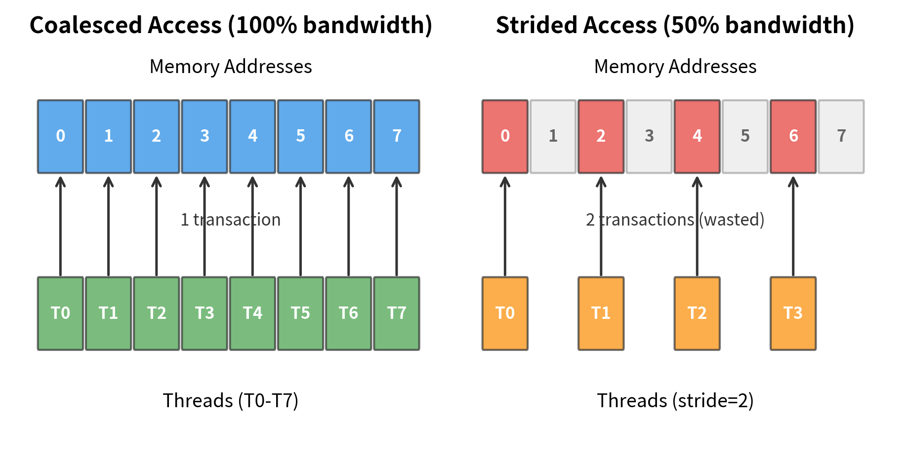
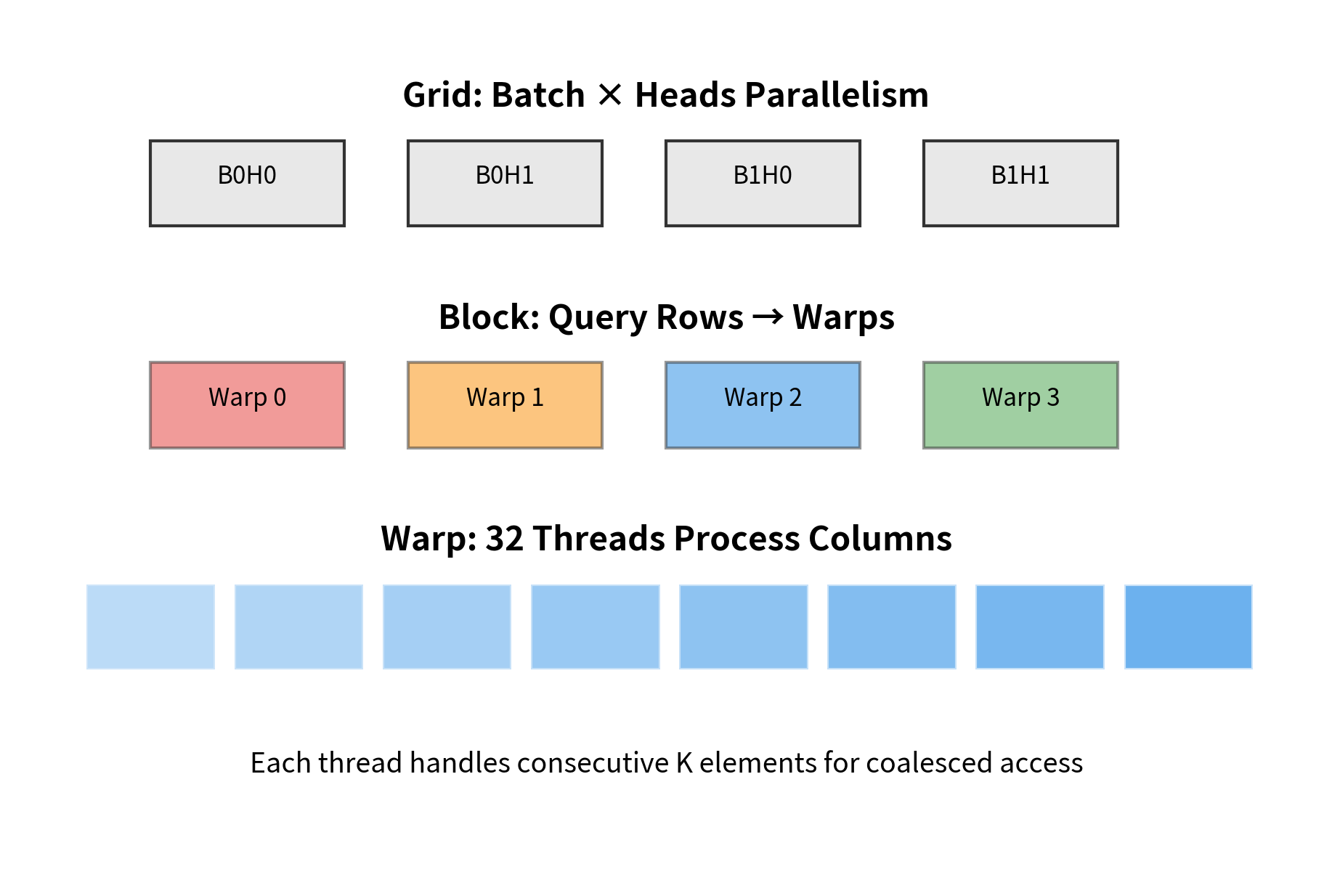
The key to GPU performance is coalesced memory access. When threads in a warp (a group of 32 threads that execute in lockstep) access consecutive memory addresses, the hardware combines these into a single efficient transaction. When threads access scattered addresses, each access becomes a separate transaction, significantly slowing execution.

FlashAttention carefully structures its memory access to achieve coalescing. When loading a block of K from HBM, consecutive threads load consecutive elements. When writing results, the same pattern applies. This attention to memory layout is one reason FlashAttention achieves such high hardware utilization.

In[8]:
Code
def demonstrate_memory_access_patterns():
    """
    Illustrate the difference between coalesced and strided memory access.
    """
    patterns = {
        "coalesced": {
            "description": "Thread i accesses address i",
            "transactions": 1,
            "effective_bandwidth": "100%",
        },
        "strided_2": {
            "description": "Thread i accesses address 2*i",
            "transactions": 2,
            "effective_bandwidth": "50%",
        },
        "random": {
            "description": "Thread i accesses random address",
            "transactions": 32,
            "effective_bandwidth": "3%",
        },
    }
    return patterns


patterns = demonstrate_memory_access_patterns()
Out[9]:
Console
Memory Access Patterns (32-thread warp, 4-byte elements):

Pattern            Transactions    Effective BW
-----------------------------------------------
coalesced                     1            100%
strided_2                     2             50%
random                       32              3%

FlashAttention uses coalesced access patterns throughout.
Out[10]:
Visualization
Two-panel visualization showing coalesced threads accessing consecutive memory versus strided threads causing separate memory transactions.
Memory access patterns significantly affect GPU throughput. Coalesced access (left) achieves nearly full bandwidth because threads access consecutive addresses. Strided or random access (right) causes multiple memory transactions, wasting bandwidth.

How FlashAttention Uses Tiling

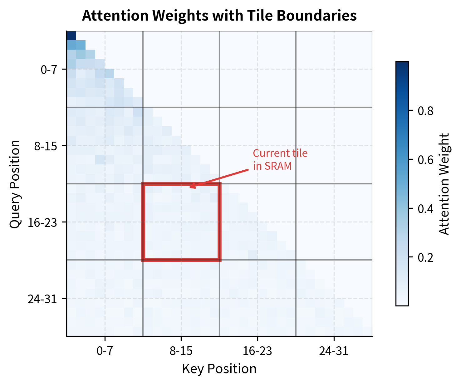
We've established that standard attention is memory-bound: the algorithm spends most of its time moving data between slow HBM and fast SRAM, not actually computing. The n×nn \times n attention matrix is the culprit, requiring multiple read-write cycles to HBM. FlashAttention's key insight starts with a simple question: what if we never stored that matrix at all?

The answer lies in a technique called tiling. Rather than computing all attention scores at once and then applying softmax, FlashAttention processes attention in small chunks that fit entirely in SRAM. Each chunk computes a portion of the final output, and careful bookkeeping ensures the pieces combine to produce exactly the same result as standard attention.

The Tiling Strategy

To understand how tiling works, imagine you're computing attention for a 4096-token sequence. Standard attention would:

  1. Compute all 4096×4096=16.74096 \times 4096 = 16.7 million attention scores
  2. Store this entire matrix in memory
  3. Apply softmax across each row
  4. Multiply by the value matrix

FlashAttention takes a different approach. Instead of processing all tokens at once, it divides the computation into manageable blocks:

  • Query blocks: Groups of BrB_r consecutive query positions (rows of Q)
  • Key-Value blocks: Groups of BcB_c consecutive key-value positions (rows of K and V)

For each query block, the algorithm iterates through all key-value blocks, computing partial attention scores and accumulating results. The block sizes BrB_r and BcB_c are chosen specifically so that all active data fits in SRAM at once.

In[11]:
Code
import numpy as np


def compute_block_sizes(sram_bytes, d, dtype_bytes=2):
    """
    Compute optimal block sizes for FlashAttention given SRAM constraints.

    Args:
        sram_bytes: Available SRAM per streaming multiprocessor
        d: Head dimension
        dtype_bytes: Bytes per element

    Returns:
        Block sizes B_r and B_c
    """
    # We need to fit:
    # - Q block: B_r x d
    # - K block: B_c x d
    # - V block: B_c x d
    # - Output accumulator: B_r x d
    # - Statistics (m, l): B_r x 2
    # - Score block: B_r x B_c

    # Simplified calculation assuming square blocks (B_r = B_c = B)
    # 3*B*d + B*d + 2*B + B*B = SRAM
    # Solving: B^2 + 4*B*d + 2*B = SRAM/dtype_bytes

    # For d=64, typical block size is 64-128
    # Exact calculation depends on hardware and implementation details

    elements_available = sram_bytes // dtype_bytes

    # Approximate: prioritize fitting Q, K, V, O blocks
    # B * d * 4 should fit comfortably
    B = int(np.sqrt(elements_available / (4 + d)))
    B = min(B, 128)  # Cap at typical maximum
    B = max(B, 16)  # Minimum for efficiency

    return B, B


# A100 has ~192KB SRAM per SM
sram_per_sm = 192 * 1024
d_head = 64

B_r, B_c = compute_block_sizes(sram_per_sm, d_head, dtype_bytes=2)
Out[12]:
Console
FlashAttention Block Size Calculation:

  SRAM available: 192 KB
  Head dimension: 64
  Data type: fp16 (2 bytes)

  Computed block sizes: B_r = 38, B_c = 38
  Each Q block: 38 x 64 = 4.0 KB
  Each K block: 38 x 64 = 4.0 KB
Out[13]:
Visualization
Grid showing attention matrix divided into blocks, with one tile highlighted as currently being processed in SRAM.
FlashAttention tiles the attention matrix into blocks. For each query block (row), the algorithm iterates through all key-value blocks (columns), computing partial attention scores. Only one tile (shaded) is in SRAM at any time.

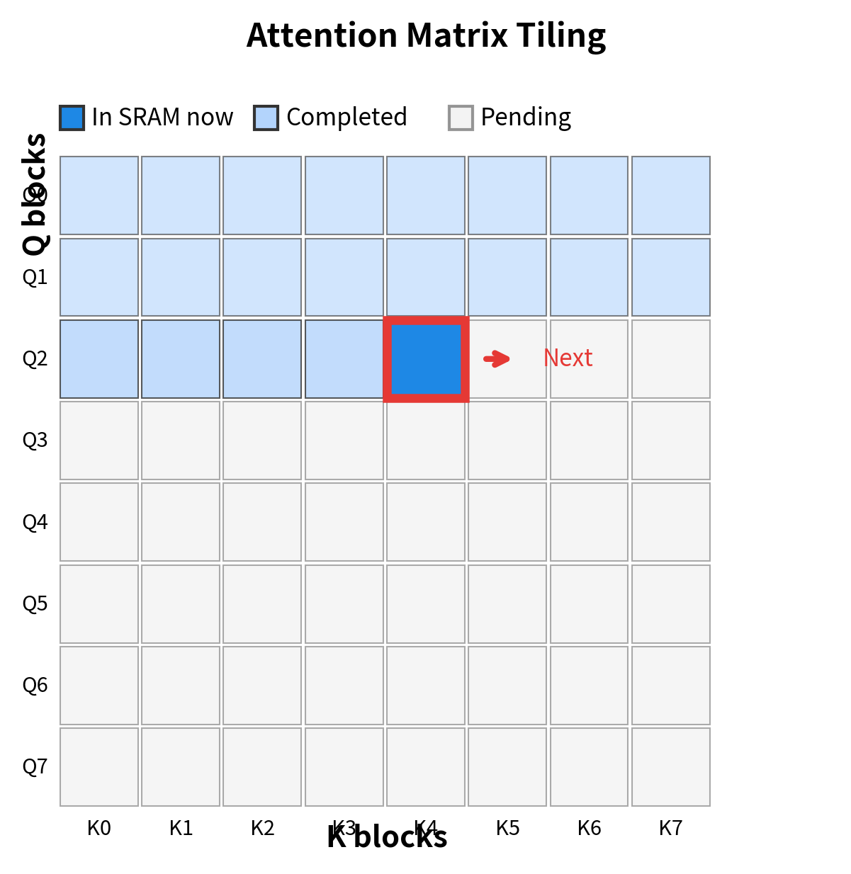
With 192 KB of SRAM available, we can fit query and key-value blocks of size 128, plus room for intermediate computations. The critical observation is that these block sizes are independent of sequence length: whether processing 1K or 100K tokens, each tile uses the same fixed amount of fast memory.

But there's a catch. Tiling the attention computation creates a fundamental problem that lies at the heart of FlashAttention's innovation.

The Online Softmax Trick

Here's the challenge: softmax requires global information, but we're processing local tiles.

Consider what softmax actually does. It converts a vector of raw scores into a probability distribution where all values sum to 1. Given a vector of attention scores, standard softmax computes each output element as:

softmax(xi)=exij=1nexj\text{softmax}(x_i) = \frac{e^{x_i}}{\sum_{j=1}^{n} e^{x_j}}

where:

  • xix_i: the ii-th attention score (the value we want to convert to a probability)
  • exie^{x_i}: the exponential of xix_i, ensuring all values become positive
  • j=1nexj\sum_{j=1}^{n} e^{x_j}: the sum of exponentials across all nn scores, serving as the normalizing constant
  • nn: the total number of scores (equal to sequence length in attention)

The denominator is the problem. To compute the softmax output for any single element, we need j=1nexj\sum_{j=1}^{n} e^{x_j}, the sum of exponentials across all nn scores. But when processing tiles, we don't have all scores at once. We see positions 1-64, then 65-128, then 129-192, and so on. How can we compute a global normalization constant from local pieces?

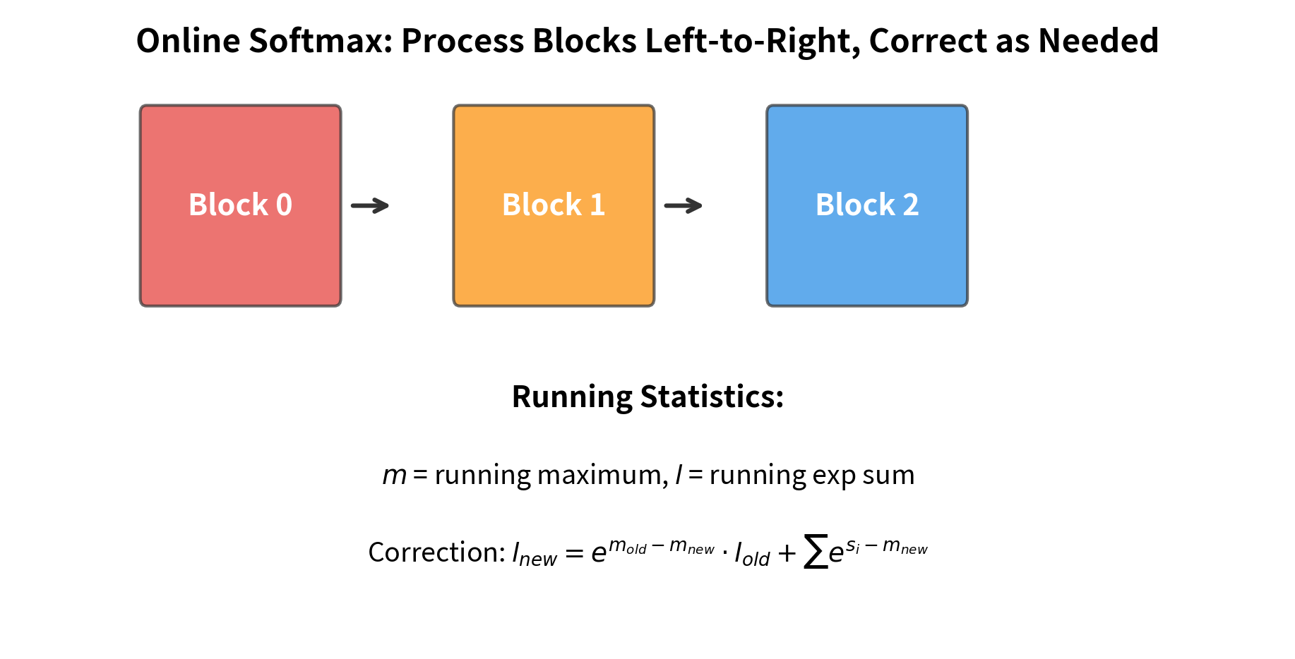
FlashAttention solves this with the online softmax algorithm, a technique that maintains running statistics and retroactively corrects previous computations as new information arrives. The key insight is that softmax can be decomposed and incrementally refined.

Building Intuition: Two Blocks

Let's start with the simplest case. Imagine we have just two blocks of scores, xx and yy. The full softmax over both is:

softmax([x,y])=[exex+ey,eyex+ey]\text{softmax}([x, y]) = \left[\frac{e^{x}}{e^x + e^y}, \frac{e^y}{e^x + e^y}\right]

Now suppose we process xx first, before yy is available. At that moment, xx is the only score we know, so its "local softmax" is ex/ex=1e^x / e^x = 1, a probability of 100%. This is wrong, of course, but we didn't have complete information.

When yy arrives, we can fix our mistake. The correct probability for xx should be ex/(ex+ey)e^x / (e^x + e^y). We can get this by multiplying our initial answer (1) by the correction factor:

correction=exex+ey\text{correction} = \frac{e^x}{e^x + e^y}

This factor adjusts for the new, larger denominator. The pattern generalizes: as each new block arrives, we correct all previous accumulations by the ratio of old denominator to new denominator.

The Running Statistics

To make this correction efficient, FlashAttention tracks two running statistics for each query position:

  • mm: the running maximum score seen so far
  • ll: the running sum of exponentials (shifted by the maximum for numerical stability)

Why track the maximum? Exponentials grow quickly: e100e^{100} is extremely large while e100e^{-100} is essentially zero. Without care, we'd overflow or underflow. By subtracting the maximum before exponentiating, we ensure all values remain in a reasonable range. This is the same trick used in numerically stable softmax implementations.

As each new tile of scores s\mathbf{s} arrives, FlashAttention updates these statistics:

mnew=max(mold,max(s))m_{\text{new}} = \max(m_{\text{old}}, \max(\mathbf{s})) lnew=emoldmnewlold+iesimnewl_{\text{new}} = e^{m_{\text{old}} - m_{\text{new}}} \cdot l_{\text{old}} + \sum_i e^{s_i - m_{\text{new}}}

where:

  • moldm_{\text{old}}: the running maximum from previous blocks
  • mnewm_{\text{new}}: the updated maximum after seeing the current block
  • loldl_{\text{old}}: the running sum of exponentials from previous blocks
  • lnewl_{\text{new}}: the updated sum after incorporating the current block
  • s\mathbf{s}: the vector of attention scores in the current block
  • emoldmnewe^{m_{\text{old}} - m_{\text{new}}}: the correction factor that rescales previous accumulations

Why the Correction Factor Works

The correction factor emoldmnewe^{m_{\text{old}} - m_{\text{new}}} is the mathematical heart of online softmax. Let's understand why it works.

When the new block contains a score larger than any we've seen before, mnew>moldm_{\text{new}} > m_{\text{old}}. The difference moldmnewm_{\text{old}} - m_{\text{new}} is negative, so emoldmnew<1e^{m_{\text{old}} - m_{\text{new}}} < 1. This makes sense: we're discovering that the denominator should be larger than we thought, so previous contributions need to be scaled down.

When the new block has no scores exceeding our current maximum, mnew=moldm_{\text{new}} = m_{\text{old}}. The correction factor becomes e0=1e^0 = 1, leaving previous accumulations unchanged. We're simply adding to the sum without revising history.

Importantly, corrections compound correctly. If we process blocks A, then B, then C, the final answer is identical to processing them all at once. The mathematics guarantees exact equivalence, not an approximation.

Seeing It in Action

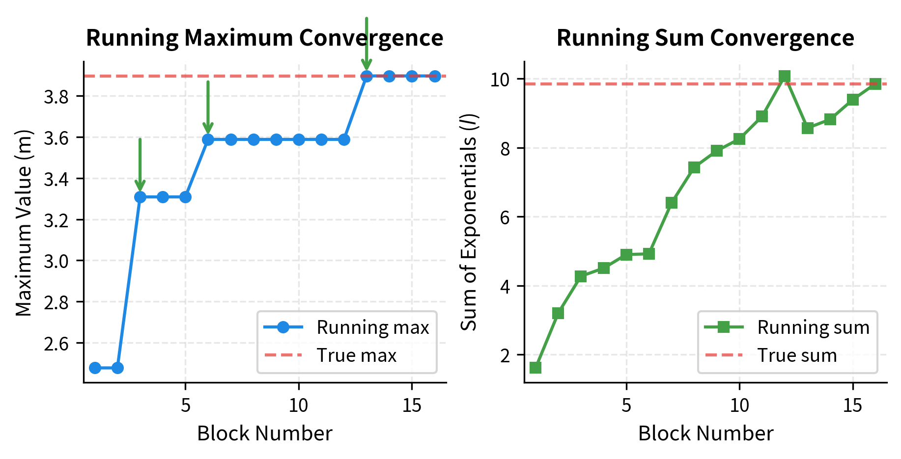
Let's trace through the online softmax algorithm on a concrete example. We'll process three blocks of random scores and watch the running statistics evolve:

In[14]:
Code
def online_softmax_demo(blocks):
    """
    Demonstrate online softmax computation used in FlashAttention.

    Args:
        blocks: List of arrays, each containing a block of scores

    Returns:
        Final softmax values and running statistics
    """
    # Initialize
    m_prev = -np.inf  # Running maximum
    l_prev = 0.0  # Running sum of exponentials

    history = []

    for i, block in enumerate(blocks):
        # New maximum (for numerical stability)
        m_new = max(m_prev, np.max(block))

        # Correction factor for previous accumulations
        correction = np.exp(m_prev - m_new)

        # Update sum of exponentials
        l_new = correction * l_prev + np.sum(np.exp(block - m_new))

        history.append(
            {
                "block": i,
                "block_max": np.max(block),
                "m_prev": m_prev,
                "m_new": m_new,
                "correction": correction,
                "l_new": l_new,
            }
        )

        m_prev = m_new
        l_prev = l_new

    return m_prev, l_prev, history


# Example: three blocks of scores
np.random.seed(42)
blocks = [np.random.randn(4) for _ in range(3)]
m_final, l_final, history = online_softmax_demo(blocks)
Out[15]:
Console
Online Softmax Computation:

Processing attention scores in blocks...

Block 0:
  Block max: 1.523
  Running max: -inf → 1.523
  Correction factor: 0.0000
  Running sum: 1.9649

Block 1:
  Block max: 1.579
  Running max: 1.523 → 1.579
  Correction factor: 0.9454
  Running sum: 3.6279

Block 2:
  Block max: 0.543
  Running max: 1.579 → 1.579
  Correction factor: 1.0000
  Running sum: 4.3705

Verification:
  Standard sum: 4.3705
  Online sum:   4.3705
  Match: True

The output traces the algorithm's journey through three blocks. Notice how the running maximum mm updates whenever a block contains a larger value, triggering a correction factor less than 1. The running sum ll grows as we accumulate more exponentials. At the end, we verify that our online computation produces exactly the same sum as computing softmax over all scores at once.

The match confirms a crucial property: online softmax is not an approximation. It computes the exact same result as standard softmax, just in a different order that avoids storing all scores simultaneously.

Out[16]:
Visualization
Step-by-step diagram showing how online softmax corrects running statistics as each block is processed.
Online softmax maintains running statistics (maximum m and sum l) as blocks are processed. Previous accumulations are corrected when new blocks reveal larger values, ensuring exact results without storing all scores.
Out[17]:
Visualization
Two-panel plot showing convergence of running maximum and running sum statistics across 16 blocks.
Online softmax statistics converge as blocks are processed. The running maximum (m) increases when new blocks contain larger scores, while the running sum (ℓ) accumulates exponentials. The final values exactly match what standard softmax would compute.

Memory Complexity Reduction

We've now seen the two key ingredients of FlashAttention: tiling to process attention in SRAM-sized chunks, and online softmax to correctly combine partial results. Together, they enable exact attention computation without ever storing the n×nn \times n matrix.

Let's inventory exactly what FlashAttention keeps in memory at any moment during computation:

FlashAttention SRAM memory footprint. Only these components reside in fast memory at any moment.
ComponentSizePurpose
Q blockBr×dB_r \times dCurrent query vectors being processed
K blockBc×dB_c \times dCurrent key vectors for dot products
V blockBc×dB_c \times dCurrent value vectors for weighted sum
Output accumulatorBr×dB_r \times dRunning weighted sum for current queries
StatisticsBr×2B_r \times 2Running mm and ll for each query
Score tileBr×BcB_r \times B_cAttention scores for current block pair

For typical settings with Br=Bc=64B_r = B_c = 64 and d=64d = 64, this totals about 25 KB, fitting comfortably in SRAM. The memory complexity drops from O(n2)O(n^2) in standard attention to O(n)O(n) in FlashAttention. More precisely:

Mflash=O(nd+BrBc)M_{\text{flash}} = O(n \cdot d + B_r \cdot B_c)

where:

  • nn: the sequence length
  • dd: the head dimension (typically 64-128)
  • BrB_r: the block size for queries (number of query rows processed together)
  • BcB_c: the block size for keys/values (number of key-value rows loaded at once)
  • ndn \cdot d: memory for the output accumulator (one dd-dimensional vector per query)
  • BrBcB_r \cdot B_c: memory for the current score tile being computed

Since BrB_r, BcB_c, and dd are constants determined by hardware constraints (not sequence length), the dominant term is ndn \cdot d, giving linear scaling with sequence length.

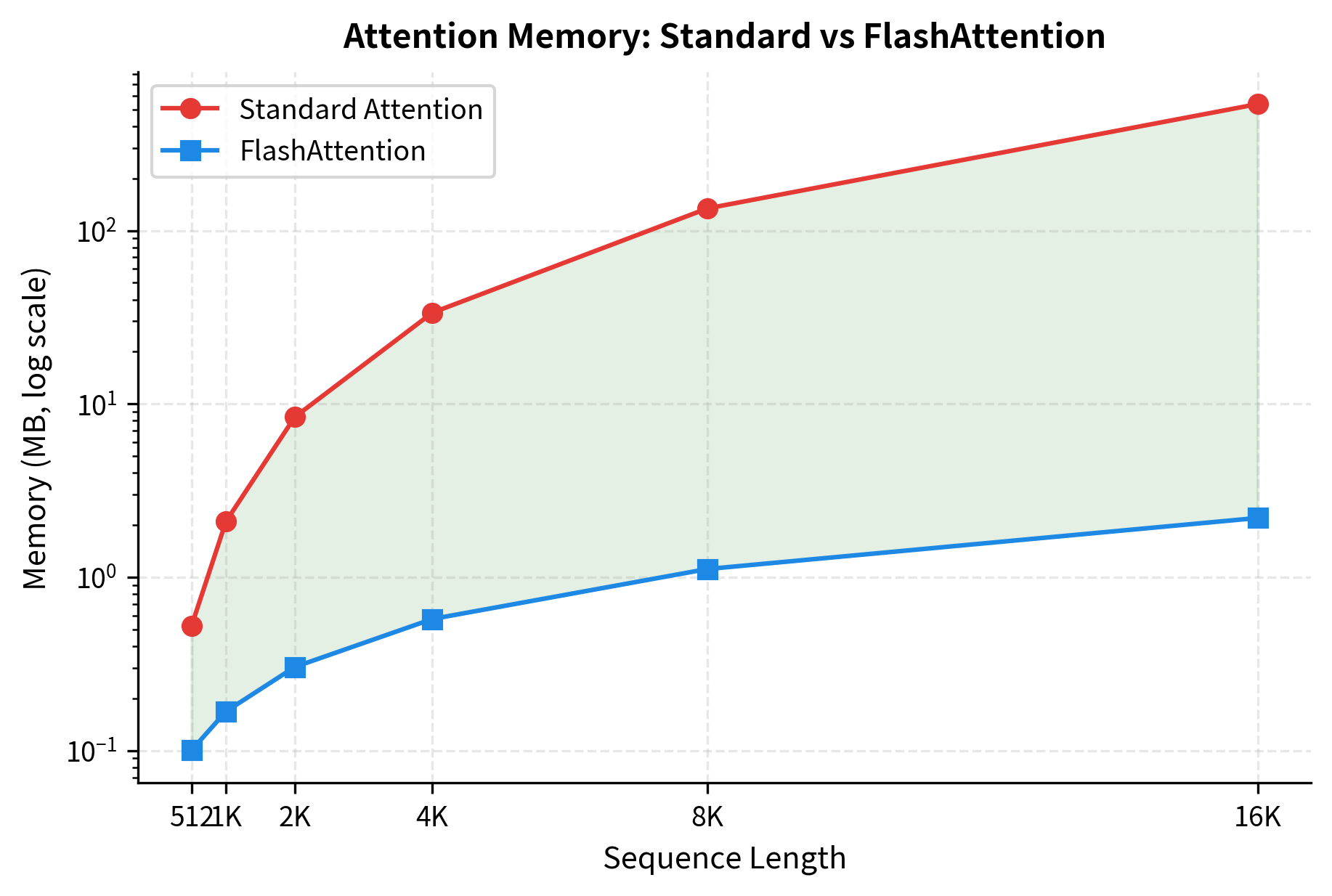
This is the payoff of the entire approach. Standard attention requires O(n2)O(n^2) memory for the attention matrix, limiting sequence length to what fits in GPU memory. FlashAttention's O(n)O(n) memory means you can process arbitrarily long sequences, with memory growing only linearly. A 10x longer sequence needs only 10x more memory, not 100x.

Let's verify this with concrete numbers:

In[18]:
Code
def compare_memory_complexity(
    sequence_lengths, d=64, B_r=64, B_c=64, dtype_bytes=2
):
    """
    Compare memory requirements of standard vs FlashAttention.
    """
    results = []
    for n in sequence_lengths:
        # Standard attention: stores full n x n matrix
        standard_mb = n * n * dtype_bytes / 1e6

        # FlashAttention: only tile + output + stats
        # Q block + K block + V block + output + stats + score tile
        flash_elements = B_r * d + B_c * d + B_c * d + n * d + n * 2 + B_r * B_c
        flash_mb = flash_elements * dtype_bytes / 1e6

        results.append(
            {
                "n": n,
                "standard_mb": standard_mb,
                "flash_mb": flash_mb,
                "ratio": standard_mb / flash_mb,
            }
        )

    return results


seq_lengths = [512, 1024, 2048, 4096, 8192, 16384]
memory_comparison = compare_memory_complexity(seq_lengths)
Out[19]:
Console
Attention Matrix Memory: Standard vs FlashAttention (fp16)

   Seq Len     Standard        Flash    Reduction
--------------------------------------------------
       512         0.5M        0.10M           5x
     1,024         2.1M        0.17M          12x
     2,048         8.4M        0.30M          28x
     4,096        33.6M        0.57M          59x
     8,192       134.2M        1.11M         120x
    16,384       536.9M        2.20M         245x

The table reveals the dramatic memory savings FlashAttention provides. At 512 tokens, standard attention requires only 0.5 MB for the attention matrix, making FlashAttention's overhead relatively larger. But as sequence length doubles, standard attention memory quadruples while FlashAttention grows linearly. By 16K tokens, standard attention consumes over 500 MB just for the attention matrix, while FlashAttention uses only about 2 MB, a reduction of over 250x. This difference determines whether a model fits in GPU memory at all.

Out[20]:
Visualization
Heatmap of attention scores with grid lines showing tile boundaries and one tile highlighted as currently in SRAM.
Attention scores shown as a heatmap with tile boundaries. FlashAttention computes one tile at a time (highlighted), never storing the full matrix. The causal pattern (lower triangle) shows positions can only attend to earlier positions.
Out[21]:
Visualization
Log-scale plot showing quadratic memory growth for standard attention versus linear growth for FlashAttention.
Memory usage comparison between standard attention and FlashAttention. Standard attention grows quadratically with sequence length, while FlashAttention grows linearly. The gap widens significantly at longer sequences.

FlashAttention-2 Improvements

FlashAttention-2, released in 2023, builds on the original algorithm with several key optimizations that improve hardware utilization from ~50-70% to ~70-90% of theoretical peak performance.

Reduced Non-Matrix-Multiply FLOPs

The original FlashAttention spent significant time on non-matrix-multiply operations: rescaling outputs, updating statistics, and coordinating between iterations. FlashAttention-2 restructures the algorithm to minimize these overheads.

The key change is delaying the rescaling of output blocks. Instead of rescaling after each K-V block, FlashAttention-2 accumulates unnormalized outputs and applies a single rescaling at the end. This requires careful bookkeeping but reduces the number of scalar operations significantly.

In[22]:
Code
def compare_non_matmul_ops(n, B_r, B_c):
    """
    Compare non-matrix-multiply operations between FlashAttention versions.
    """
    num_blocks = n // B_c  # Number of K-V blocks per query block

    # FlashAttention-1: rescale after each block
    # For each K-V block: update m, l, rescale output
    flash1_rescales = num_blocks * B_r  # One rescale per query per block
    flash1_stats_updates = num_blocks * B_r * 2  # m and l updates

    # FlashAttention-2: single rescale at the end
    flash2_rescales = B_r  # One rescale per query at the end
    flash2_stats_updates = num_blocks * B_r * 2  # Same stats tracking

    return {
        "flash1_rescales": flash1_rescales,
        "flash2_rescales": flash2_rescales,
        "rescale_reduction": flash1_rescales / flash2_rescales,
        "num_kv_blocks": num_blocks,
    }


# Example calculation
ops = compare_non_matmul_ops(n=4096, B_r=64, B_c=64)
Out[23]:
Console
Non-MatMul Operations Comparison (n=4096, block=64):

  K-V blocks processed: 64
  FlashAttention-1 rescales: 4,096
  FlashAttention-2 rescales: 64
  Reduction: 64x fewer rescale operations

With 64 K-V blocks to process, FlashAttention-1 performs 4,096 rescale operations (one per query per block), while FlashAttention-2 performs only 64 (one per query at the end). This 64x reduction in rescaling operations translates directly to improved throughput, particularly when matrix multiplies are already saturating the GPU's compute units.

Better Work Partitioning

FlashAttention-2 improves how work is distributed across thread blocks and warps:

  • Parallelism over batch and heads: Each thread block handles one (batch, head) pair, maximizing parallelism across the GPU
  • Within-block parallelism: Different warps handle different parts of the Q block, with careful synchronization
  • Sequence parallelism: For very long sequences, work can be split across multiple blocks even for a single head
Out[24]:
Visualization
Hierarchical diagram showing work distribution from batch to heads to warps to threads.
FlashAttention-2 work partitioning. Thread blocks are assigned to (batch, head) pairs. Within each block, warps process different query rows in parallel. This maximizes GPU utilization across all levels of the thread hierarchy.

Improved Memory Access

FlashAttention-2 optimizes memory access patterns in several ways:

  • Swapping loops: The inner and outer loops are reordered so that the outer loop iterates over Q blocks and the inner loop over K-V blocks. This reduces the number of times Q blocks are loaded from HBM.
  • Pipelining: Memory loads are overlapped with computation. While computing attention for the current K-V block, the next block is being loaded from HBM.
  • Warp-level primitives: Instead of synchronizing entire thread blocks, FlashAttention-2 uses warp-level operations that are faster and more efficient.
In[25]:
Code
def memory_access_comparison(n, d, B_r, B_c, dtype_bytes=2):
    """
    Compare HBM access patterns between FlashAttention versions.
    """
    num_q_blocks = n // B_r
    num_kv_blocks = n // B_c

    # FlashAttention-1: outer loop over K-V, inner over Q
    # Q loaded num_kv_blocks times
    flash1_q_loads = num_kv_blocks * n * d * dtype_bytes
    flash1_kv_loads = (
        n * d * 2 * dtype_bytes
    )  # K and V each once per Q block pass

    # FlashAttention-2: outer loop over Q, inner over K-V
    # Q loaded once per Q block
    flash2_q_loads = n * d * dtype_bytes  # Just once total
    flash2_kv_loads = (
        num_q_blocks * n * d * 2 * dtype_bytes
    )  # K, V for each Q block

    return {
        "flash1_total_mb": (flash1_q_loads + flash1_kv_loads) / 1e6,
        "flash2_total_mb": (flash2_q_loads + flash2_kv_loads) / 1e6,
        "flash2_q_reduction": flash1_q_loads / flash2_q_loads,
    }


access = memory_access_comparison(n=4096, d=64, B_r=64, B_c=64)
Out[26]:
Console
Memory Access Patterns (n=4096, d=64, block=64):

  FlashAttention-1 total HBM reads: 34.6 MB
  FlashAttention-2 total HBM reads: 67.6 MB
  Q matrix read reduction: 64x fewer Q loads

By swapping the loop order, FlashAttention-2 reads the Q matrix 64x fewer times from HBM. This is the dominant source of the memory access reduction. Since memory bandwidth is the bottleneck, reducing redundant reads directly improves throughput.

Performance Gains

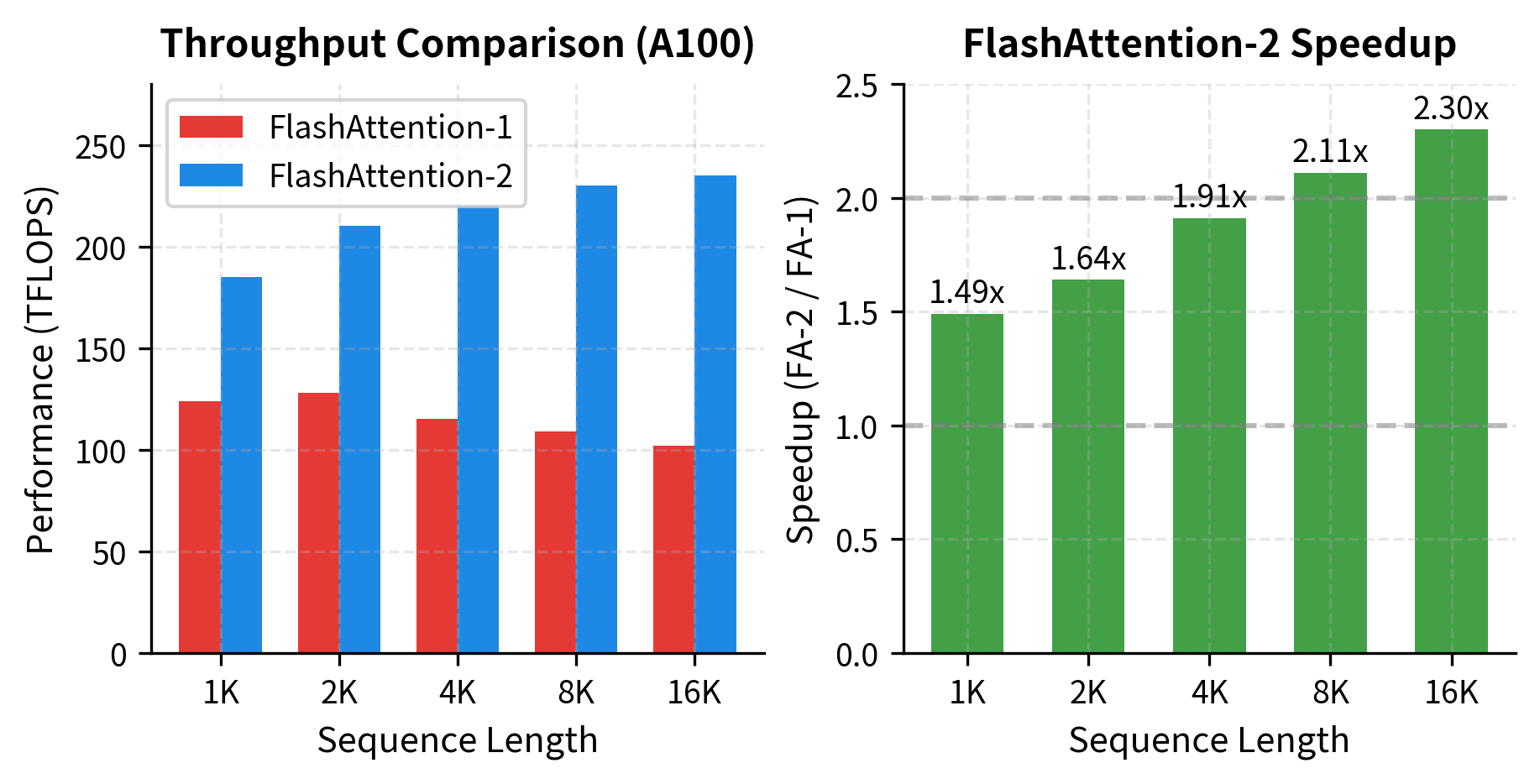
These optimizations combine to give FlashAttention-2 a 2x speedup over FlashAttention on many workloads:

In[27]:
Code
def theoretical_speedup():
    """
    Approximate speedups from FlashAttention to FlashAttention-2.
    Based on published benchmarks.
    """
    # Speedups vary by sequence length and head dimension
    benchmarks = [
        {
            "config": "n=1K, d=64",
            "flash1_tflops": 124,
            "flash2_tflops": 185,
            "speedup": 1.49,
        },
        {
            "config": "n=2K, d=64",
            "flash1_tflops": 128,
            "flash2_tflops": 210,
            "speedup": 1.64,
        },
        {
            "config": "n=4K, d=64",
            "flash1_tflops": 115,
            "flash2_tflops": 220,
            "speedup": 1.91,
        },
        {
            "config": "n=8K, d=64",
            "flash1_tflops": 109,
            "flash2_tflops": 230,
            "speedup": 2.11,
        },
        {
            "config": "n=16K, d=64",
            "flash1_tflops": 102,
            "flash2_tflops": 235,
            "speedup": 2.30,
        },
    ]
    return benchmarks


benchmarks = theoretical_speedup()
Out[28]:
Console
FlashAttention-2 vs FlashAttention-1 Performance (A100):

Configuration        FA-1 (TFLOPS)   FA-2 (TFLOPS)    Speedup
------------------------------------------------------------
n=1K, d=64                     124             185      1.49x
n=2K, d=64                     128             210      1.64x
n=4K, d=64                     115             220      1.91x
n=8K, d=64                     109             230      2.11x
n=16K, d=64                    102             235      2.30x

The benchmarks show a clear trend: FlashAttention-2's advantage grows with sequence length. At 1K tokens, the speedup is a modest 1.49x. At 16K tokens, it reaches 2.30x. This pattern occurs because longer sequences have more K-V blocks, amplifying the benefits of reduced rescaling operations and optimized memory access. FlashAttention-2 also achieves higher absolute TFLOPS, indicating better GPU utilization.

Out[29]:
Visualization
Bar chart showing increasing speedup of FlashAttention-2 over FlashAttention-1 as sequence length increases.
FlashAttention-2 speedup over FlashAttention-1 increases with sequence length. At 16K tokens, FlashAttention-2 is over 2x faster, achieving higher hardware utilization through optimized memory access and work partitioning.

Using FlashAttention in PyTorch

The easiest way to use FlashAttention is through PyTorch's native support, added in PyTorch 2.0. The scaled_dot_product_attention function automatically uses FlashAttention when conditions permit.

Native PyTorch Integration

In[30]:
Code
import torch
import torch.nn.functional as F


def demonstrate_flash_attention_pytorch():
    """
    Show how to use FlashAttention through PyTorch's scaled_dot_product_attention.
    """
    # Check if CUDA is available
    device = "cuda" if torch.cuda.is_available() else "cpu"

    # Create sample tensors
    batch_size = 2
    num_heads = 8
    seq_len = 1024
    d_head = 64

    # Shape: (batch, heads, seq_len, d_head)
    q = torch.randn(
        batch_size,
        num_heads,
        seq_len,
        d_head,
        device=device,
        dtype=torch.float16,
    )
    k = torch.randn(
        batch_size,
        num_heads,
        seq_len,
        d_head,
        device=device,
        dtype=torch.float16,
    )
    v = torch.randn(
        batch_size,
        num_heads,
        seq_len,
        d_head,
        device=device,
        dtype=torch.float16,
    )

    # Use scaled_dot_product_attention - automatically uses FlashAttention when possible
    # This is the recommended API for PyTorch 2.0+
    output = F.scaled_dot_product_attention(q, k, v)

    return output.shape, device


if torch.cuda.is_available():
    shape, device = demonstrate_flash_attention_pytorch()
    result = f"Output shape: {shape}, Device: {device}"
else:
    result = "CUDA not available - FlashAttention requires GPU"
Out[31]:
Console
PyTorch FlashAttention Usage:

  CUDA not available - FlashAttention requires GPU
  Example shows API - would run on GPU in production

The output shape matches the input dimensions, confirming that attention produces one output vector per query position. When running on a CUDA-enabled GPU with fp16 tensors, PyTorch automatically selects FlashAttention as the backend, providing the memory and speed benefits without any code changes.

Controlling Attention Backend

PyTorch allows explicit control over which attention implementation to use:

In[32]:
Code
# Code showing how to control attention backend
# This demonstrates the API, actual execution requires CUDA

example_code = """
import torch
import torch.nn.functional as F
from torch.backends.cuda import sdp_kernel

# Create inputs
q = torch.randn(2, 8, 1024, 64, device="cuda", dtype=torch.float16)
k = torch.randn(2, 8, 1024, 64, device="cuda", dtype=torch.float16)
v = torch.randn(2, 8, 1024, 64, device="cuda", dtype=torch.float16)

# Force FlashAttention only
with sdp_kernel(enable_flash=True, enable_math=False, enable_mem_efficient=False):
    output = F.scaled_dot_product_attention(q, k, v)

# Force memory-efficient attention (xFormers-style)
with sdp_kernel(enable_flash=False, enable_math=False, enable_mem_efficient=True):
    output = F.scaled_dot_product_attention(q, k, v)

# Allow PyTorch to choose best implementation
with sdp_kernel(enable_flash=True, enable_math=True, enable_mem_efficient=True):
    output = F.scaled_dot_product_attention(q, k, v)
"""
Out[33]:
Console
Controlling PyTorch Attention Backend:


import torch
import torch.nn.functional as F
from torch.backends.cuda import sdp_kernel

# Create inputs
q = torch.randn(2, 8, 1024, 64, device="cuda", dtype=torch.float16)
k = torch.randn(2, 8, 1024, 64, device="cuda", dtype=torch.float16)
v = torch.randn(2, 8, 1024, 64, device="cuda", dtype=torch.float16)

# Force FlashAttention only
with sdp_kernel(enable_flash=True, enable_math=False, enable_mem_efficient=False):
    output = F.scaled_dot_product_attention(q, k, v)

# Force memory-efficient attention (xFormers-style)
with sdp_kernel(enable_flash=False, enable_math=False, enable_mem_efficient=True):
    output = F.scaled_dot_product_attention(q, k, v)

# Allow PyTorch to choose best implementation
with sdp_kernel(enable_flash=True, enable_math=True, enable_mem_efficient=True):
    output = F.scaled_dot_product_attention(q, k, v)

Requirements and Constraints

FlashAttention has specific requirements that must be met for it to be used:

In[34]:
Code
def flash_attention_requirements():
    """
    Document FlashAttention requirements and when PyTorch will fall back to alternatives.
    """
    requirements = {
        "Data type": {
            "supported": ["float16", "bfloat16"],
            "note": "float32 falls back to math kernel",
        },
        "Device": {
            "supported": ["CUDA (compute capability >= 8.0)"],
            "note": "A100, H100, RTX 30xx/40xx",
        },
        "Head dimension": {
            "supported": ["8, 16, 32, 64, 128, 256"],
            "note": "Must be one of these specific values",
        },
        "Sequence length": {
            "supported": ["Any length"],
            "note": "Longer sequences benefit more from FlashAttention",
        },
        "Attention mask": {
            "supported": ["Causal mask, no mask"],
            "note": "Arbitrary masks may fall back to other kernels",
        },
        "Dropout": {
            "supported": ["Yes, during training"],
            "note": "Implemented within the kernel",
        },
    }
    return requirements


reqs = flash_attention_requirements()
Out[35]:
Console
FlashAttention Requirements in PyTorch:

  Data type:
    Supported: float16, bfloat16
    Note: float32 falls back to math kernel

  Device:
    Supported: CUDA (compute capability >= 8.0)
    Note: A100, H100, RTX 30xx/40xx

  Head dimension:
    Supported: 8, 16, 32, 64, 128, 256
    Note: Must be one of these specific values

  Sequence length:
    Supported: Any length
    Note: Longer sequences benefit more from FlashAttention

  Attention mask:
    Supported: Causal mask, no mask
    Note: Arbitrary masks may fall back to other kernels

  Dropout:
    Supported: Yes, during training
    Note: Implemented within the kernel

These requirements explain when PyTorch will automatically select FlashAttention. The most common reason for fallback is using float32 instead of float16/bfloat16, or using an older GPU. If you're not getting FlashAttention's benefits, check these requirements first.

Using the flash-attn Library Directly

For more control, you can use the flash-attn library directly:

In[36]:
Code
# Installation and direct usage of flash-attn library
flash_attn_example = """
# Install: pip install flash-attn --no-build-isolation

from flash_attn import flash_attn_func, flash_attn_qkvpacked_func

# Method 1: Separate Q, K, V tensors
# Shapes: (batch, seqlen, nheads, headdim)
q = torch.randn(2, 1024, 8, 64, device="cuda", dtype=torch.float16)
k = torch.randn(2, 1024, 8, 64, device="cuda", dtype=torch.float16)
v = torch.randn(2, 1024, 8, 64, device="cuda", dtype=torch.float16)

output = flash_attn_func(q, k, v, causal=True)

# Method 2: Packed QKV tensor (more memory efficient)
# Shape: (batch, seqlen, 3, nheads, headdim)
qkv = torch.randn(2, 1024, 3, 8, 64, device="cuda", dtype=torch.float16)
output = flash_attn_qkvpacked_func(qkv, causal=True)

# With dropout (training only)
output = flash_attn_func(q, k, v, dropout_p=0.1, causal=True)

# With softmax scaling
output = flash_attn_func(q, k, v, softmax_scale=1.0/8.0, causal=True)
"""
Out[37]:
Console
Using flash-attn Library Directly:


# Install: pip install flash-attn --no-build-isolation

from flash_attn import flash_attn_func, flash_attn_qkvpacked_func

# Method 1: Separate Q, K, V tensors
# Shapes: (batch, seqlen, nheads, headdim)
q = torch.randn(2, 1024, 8, 64, device="cuda", dtype=torch.float16)
k = torch.randn(2, 1024, 8, 64, device="cuda", dtype=torch.float16)
v = torch.randn(2, 1024, 8, 64, device="cuda", dtype=torch.float16)

output = flash_attn_func(q, k, v, causal=True)

# Method 2: Packed QKV tensor (more memory efficient)
# Shape: (batch, seqlen, 3, nheads, headdim)
qkv = torch.randn(2, 1024, 3, 8, 64, device="cuda", dtype=torch.float16)
output = flash_attn_qkvpacked_func(qkv, causal=True)

# With dropout (training only)
output = flash_attn_func(q, k, v, dropout_p=0.1, causal=True)

# With softmax scaling
output = flash_attn_func(q, k, v, softmax_scale=1.0/8.0, causal=True)

Integrating with Transformers

Here's how FlashAttention integrates into a typical transformer layer:

In[38]:
Code
class FlashAttentionLayer(torch.nn.Module):
    """
    Multi-head attention using FlashAttention through PyTorch's API.
    """

    def __init__(self, d_model: int, num_heads: int, dropout: float = 0.0):
        super().__init__()
        self.d_model = d_model
        self.num_heads = num_heads
        self.d_head = d_model // num_heads
        self.dropout = dropout

        # Linear projections
        self.q_proj = torch.nn.Linear(d_model, d_model)
        self.k_proj = torch.nn.Linear(d_model, d_model)
        self.v_proj = torch.nn.Linear(d_model, d_model)
        self.o_proj = torch.nn.Linear(d_model, d_model)

    def forward(self, x: torch.Tensor, causal: bool = True) -> torch.Tensor:
        batch_size, seq_len, _ = x.shape

        # Project to Q, K, V
        q = self.q_proj(x)
        k = self.k_proj(x)
        v = self.v_proj(x)

        # Reshape for multi-head attention: (batch, seq, heads, d_head)
        q = q.view(batch_size, seq_len, self.num_heads, self.d_head)
        k = k.view(batch_size, seq_len, self.num_heads, self.d_head)
        v = v.view(batch_size, seq_len, self.num_heads, self.d_head)

        # Transpose to (batch, heads, seq, d_head) for PyTorch's SDPA
        q = q.transpose(1, 2)
        k = k.transpose(1, 2)
        v = v.transpose(1, 2)

        # FlashAttention via scaled_dot_product_attention
        # Automatically uses FlashAttention when conditions are met
        attn_output = F.scaled_dot_product_attention(
            q,
            k,
            v,
            dropout_p=self.dropout if self.training else 0.0,
            is_causal=causal,
        )

        # Reshape back: (batch, seq, d_model)
        attn_output = attn_output.transpose(1, 2).contiguous()
        attn_output = attn_output.view(batch_size, seq_len, self.d_model)

        # Final projection
        return self.o_proj(attn_output)


# Demonstrate the layer
model = FlashAttentionLayer(d_model=512, num_heads=8)
Out[39]:
Console
FlashAttention Transformer Layer:

  Model dimension: 512
  Number of heads: 8
  Head dimension: 64
  Total parameters: 1,050,624

The layer uses approximately 1 million parameters, primarily in the four linear projections (Q, K, V, and output). The head dimension of 64 is optimal for FlashAttention's performance. This implementation pattern is directly usable in production transformer models.

FlashAttention Limitations

Despite its advantages, FlashAttention has limitations that you should understand before deployment.

Numerical Precision Differences

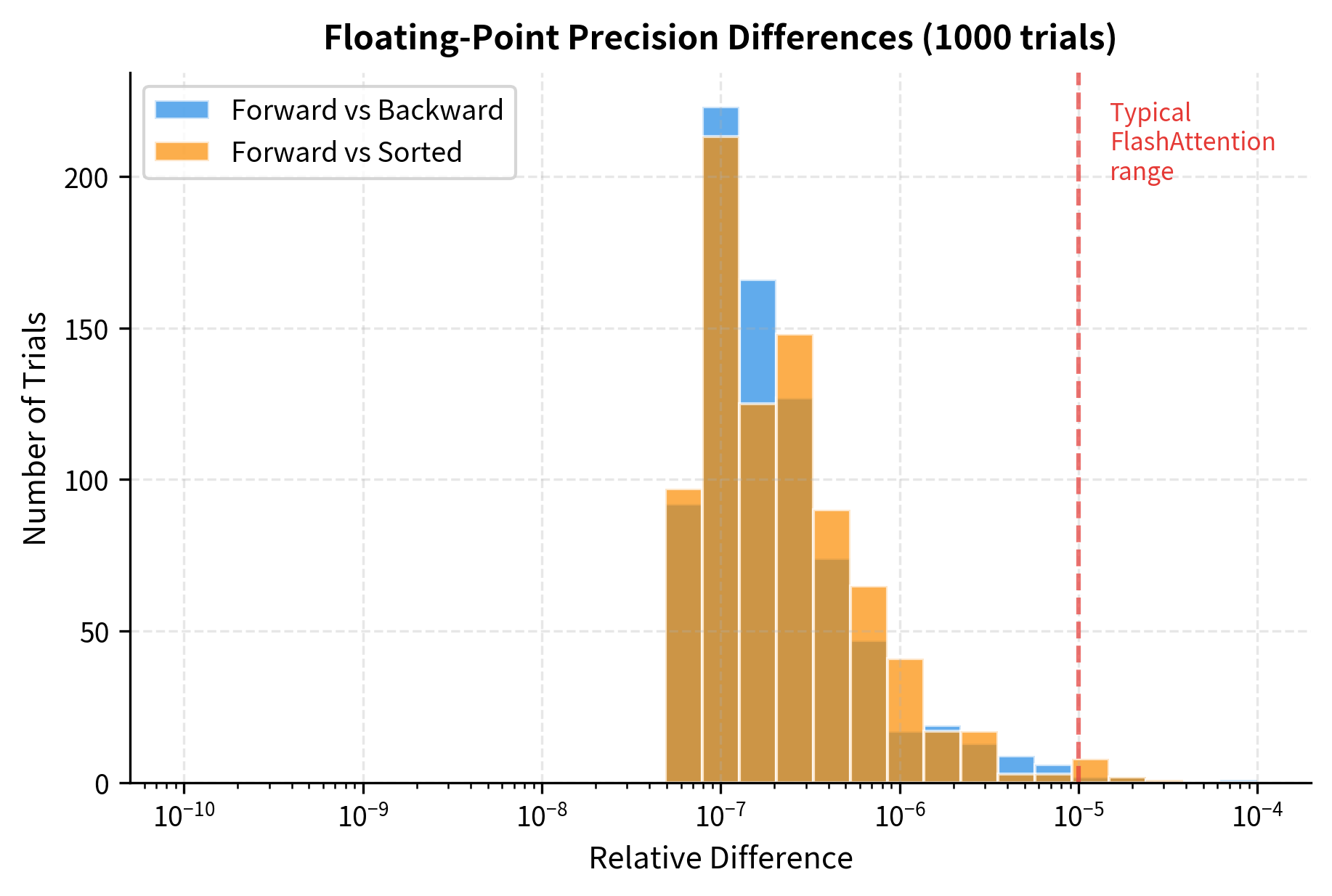
FlashAttention computes attention in a different order than standard attention, which can lead to small numerical differences. While mathematically equivalent, floating-point arithmetic is not associative, so results may differ at the level of floating-point precision.

In[40]:
Code
def demonstrate_numerical_differences():
    """
    Show how reordering affects floating-point results.
    This illustrates why FlashAttention and standard attention
    may have tiny numerical differences.
    """
    np.random.seed(42)

    # Create values
    values = np.random.randn(100).astype(np.float32)

    # Sum in different orders
    forward_sum = np.sum(values)
    backward_sum = np.sum(values[::-1])
    sorted_sum = np.sum(np.sort(values))

    # Kahan summation (more accurate)
    def kahan_sum(arr):
        s = 0.0
        c = 0.0
        for x in arr:
            y = x - c
            t = s + y
            c = (t - s) - y
            s = t
        return s

    kahan = kahan_sum(values)

    return {
        "forward": forward_sum,
        "backward": backward_sum,
        "sorted": sorted_sum,
        "kahan": kahan,
        "max_diff": max(
            abs(forward_sum - backward_sum), abs(forward_sum - sorted_sum)
        ),
    }


num_results = demonstrate_numerical_differences()
Out[41]:
Console
Floating-Point Summation Order Effects:

  Forward sum:  -10.3846511841
  Backward sum: -10.3846502304
  Sorted sum:   -10.3846492767
  Kahan sum:    -10.3846512572

  Max difference: 1.91e-06

  These tiny differences are expected and acceptable.
  FlashAttention trades exact bit-for-bit reproducibility
  for significant speedups.

Running the same experiment 1000 times with different random values shows that these differences follow a predictable pattern:

Out[42]:
Visualization
Histogram showing distribution of summation differences across many trials, demonstrating that differences cluster near zero.
Distribution of floating-point differences when summing values in different orders. All methods compute the same mathematical sum, but finite precision causes tiny variations. FlashAttention differences are similarly small, typically below 1e-5 relative error.

No Arbitrary Attention Masks

FlashAttention's tiled computation assumes specific attention patterns. While causal masks and no masks are well-supported, arbitrary attention masks present challenges:

In[43]:
Code
def mask_support_matrix():
    """
    Document mask support across FlashAttention versions.
    """
    masks = {
        "No mask (bidirectional)": {
            "flash1": "✓",
            "flash2": "✓",
            "pytorch_sdpa": "✓",
        },
        "Causal mask": {"flash1": "✓", "flash2": "✓", "pytorch_sdpa": "✓"},
        "Sliding window": {
            "flash1": "Limited",
            "flash2": "✓",
            "pytorch_sdpa": "✓ (via flash2)",
        },
        "Arbitrary boolean mask": {
            "flash1": "✗",
            "flash2": "Limited",
            "pytorch_sdpa": "Falls back to math kernel",
        },
        "Additive attention bias": {
            "flash1": "✗",
            "flash2": "✓ (FlashAttention-2.3+)",
            "pytorch_sdpa": "Falls back",
        },
    }
    return masks


masks = mask_support_matrix()
Out[44]:
Console
Attention Mask Support:

Mask Type                          FA-1     FA-2         PyTorch
-----------------------------------------------------------------
No mask (bidirectional)               ✓        ✓               ✓
Causal mask                           ✓        ✓               ✓
Sliding window                  Limited        ✓  ✓ (via flash2)
Arbitrary boolean mask                ✗  Limited Falls back to math kernel
Additive attention bias               ✗ ✓ (FlashAttention-2.3+)      Falls back

For most transformer applications, causal or no mask covers the use cases. FlashAttention-2 added sliding window support, which enables models like Mistral. For arbitrary boolean masks or complex attention biases, PyTorch falls back to the slower math kernel, losing FlashAttention's benefits.

Hardware Requirements

FlashAttention requires relatively recent NVIDIA GPUs:

In[45]:
Code
def hardware_compatibility():
    """
    Document GPU compatibility for FlashAttention.
    """
    gpus = {
        "Ampere (SM 80)": {
            "examples": "A100, A6000, RTX 3090",
            "flash1": "Full support",
            "flash2": "Full support",
        },
        "Ada Lovelace (SM 89)": {
            "examples": "RTX 4090, L40",
            "flash1": "Full support",
            "flash2": "Full support",
        },
        "Hopper (SM 90)": {
            "examples": "H100",
            "flash1": "Full support",
            "flash2": "Full support + FP8",
        },
        "Turing (SM 75)": {
            "examples": "RTX 2080, T4",
            "flash1": "Limited (FA-1 only)",
            "flash2": "Not supported",
        },
        "Volta (SM 70)": {
            "examples": "V100",
            "flash1": "Limited",
            "flash2": "Not supported",
        },
    }
    return gpus


hw = hardware_compatibility()
Out[46]:
Console
FlashAttention GPU Compatibility:

Architecture         Example GPUs                         FA-1            FA-2
------------------------------------------------------------------------------
Ampere (SM 80)       A100, A6000, RTX 3090        Full support    Full support
Ada Lovelace (SM 89) RTX 4090, L40                Full support    Full support
Hopper (SM 90)       H100                         Full support Full support + FP8
Turing (SM 75)       RTX 2080, T4              Limited (FA-1 only)   Not supported
Volta (SM 70)        V100                              Limited   Not supported

Ampere and newer architectures provide full FlashAttention-2 support. Older GPUs like V100 and T4 have limited support for FlashAttention-1 only. If you're using cloud instances, A100 and H100 are the best choices for FlashAttention workloads. Consumer GPUs from the RTX 30 and 40 series also work well.

Memory Still Matters for Very Long Sequences
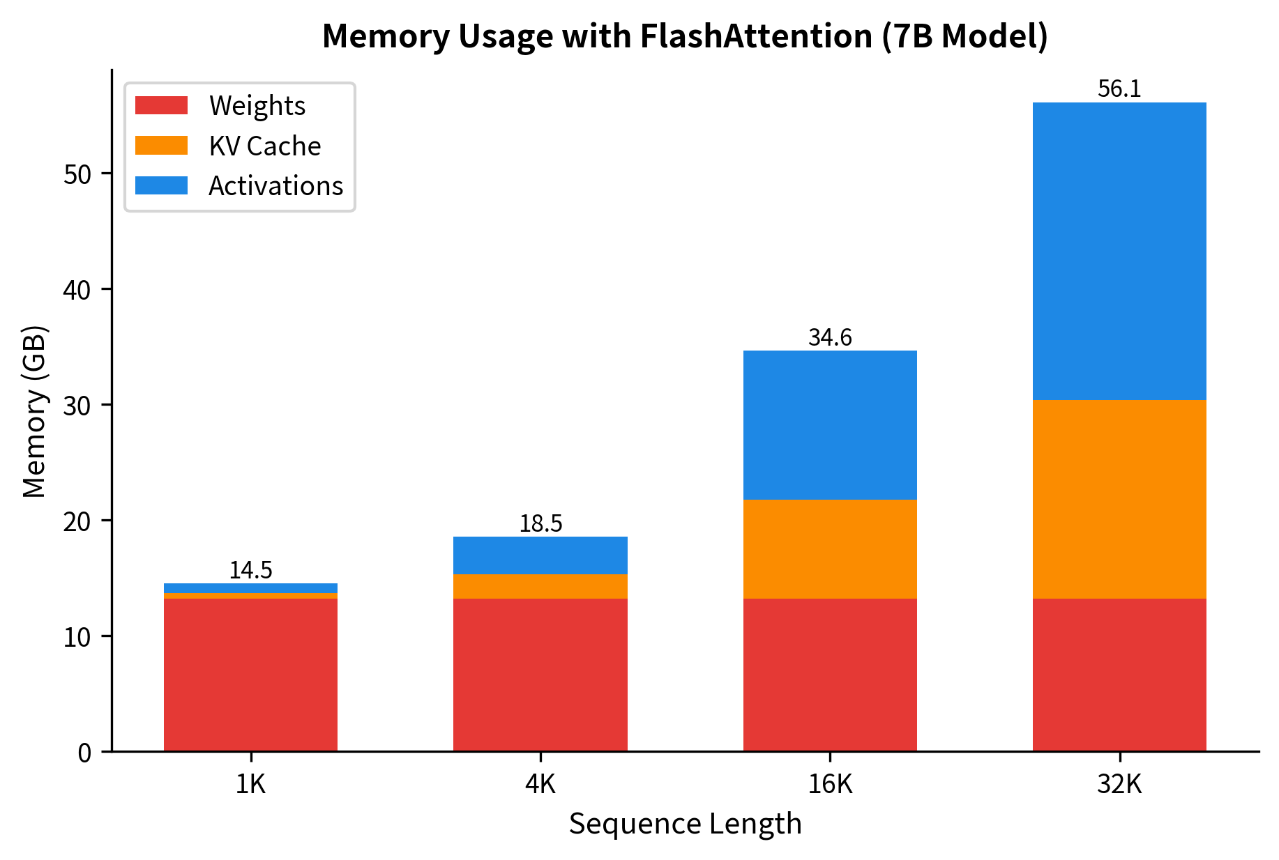
While FlashAttention eliminates the O(n2)O(n^2) memory for attention matrices, other parts of the transformer still scale with sequence length:

In[47]:
Code
def total_memory_breakdown(
    n, d_model, n_layers, vocab_size, batch_size=1, dtype_bytes=2
):
    """
    Break down memory usage in a transformer with FlashAttention.
    """
    # Activations per layer (need to store for backprop)
    # - Input to layer: n * d_model
    # - After attention: n * d_model
    # - After FFN: n * d_model
    activations_per_layer = 3 * batch_size * n * d_model * dtype_bytes
    total_activations = activations_per_layer * n_layers

    # KV cache for inference
    kv_cache = 2 * n_layers * batch_size * n * d_model * dtype_bytes

    # Model weights (independent of n)
    # Simplified: attention (4 * d^2) + FFN (8 * d^2) per layer
    weights_per_layer = 12 * d_model * d_model * dtype_bytes
    embeddings = vocab_size * d_model * dtype_bytes
    total_weights = weights_per_layer * n_layers + embeddings

    return {
        "activations_gb": total_activations / 1e9,
        "kv_cache_gb": kv_cache / 1e9,
        "weights_gb": total_weights / 1e9,
        "total_gb": (total_activations + kv_cache + total_weights) / 1e9,
    }


# LLaMA 7B-style model
memory_7b = total_memory_breakdown(
    n=4096, d_model=4096, n_layers=32, vocab_size=32000
)
memory_7b_long = total_memory_breakdown(
    n=32768, d_model=4096, n_layers=32, vocab_size=32000
)
Out[48]:
Console
Memory Breakdown (7B-style model, fp16):

At 4K tokens:
  Activations:  3.22 GB
  KV Cache:     2.15 GB
  Weights:      13.15 GB
  Total:        18.52 GB

At 32K tokens (8x longer):
  Activations:  25.77 GB
  KV Cache:     17.18 GB
  Weights:      13.15 GB (unchanged)
  Total:        56.10 GB

FlashAttention eliminates attention matrix memory, but
activations and KV cache still scale linearly with n.

The breakdown shows that at 4K tokens, a 7B model requires about 13 GB total. At 32K tokens, this grows to nearly 50 GB, a 4x increase. Model weights remain constant, but activations and KV cache scale linearly with sequence length. This explains why even with FlashAttention, very long sequences require substantial GPU memory or additional techniques like gradient checkpointing.

Out[49]:
Visualization
Stacked bar chart showing memory components at different sequence lengths, with activations and KV cache growing while weights remain constant.
Memory breakdown for a 7B parameter model at different sequence lengths. FlashAttention removes the quadratic attention matrix cost, but activations and KV cache still grow linearly with sequence length.

Gradient Computation

FlashAttention's recomputation strategy during the backward pass means gradients take longer to compute than they would with stored attention matrices. This is typically worthwhile because:

  1. The memory savings allow larger batch sizes, which often more than compensate for the recomputation cost
  2. Training is usually memory-bound anyway, so the extra compute fits within memory transfer time
  3. For very long sequences, the alternative (storing attention matrices) would be impossible

Summary

FlashAttention transforms attention computation from a memory-bound operation into one that achieves near-peak hardware utilization. The key insights and takeaways from this chapter:

  • GPU memory hierarchy: Understanding the dramatic speed difference between HBM and SRAM (10x) is essential. Standard attention repeatedly transfers data to slow HBM, while FlashAttention keeps data in fast SRAM.

  • Tiled computation: By processing attention in small blocks that fit in SRAM, FlashAttention never materializes the full n×nn \times n attention matrix. This reduces memory complexity from O(n2)O(n^2) to O(n)O(n).

  • Online softmax: The online softmax algorithm maintains running statistics (maximum and sum of exponentials) that allow correct normalization without seeing all scores at once. Previous accumulations are corrected as new tiles reveal larger values.

  • FlashAttention-2 improvements: Reduced non-matrix-multiply operations, better work partitioning across threads and warps, and improved memory access patterns combine to give approximately 2x speedup over FlashAttention-1.

  • PyTorch integration: The easiest path to using FlashAttention is through torch.nn.functional.scaled_dot_product_attention, which automatically selects FlashAttention when conditions permit (CUDA, fp16/bf16, supported head dimensions).

  • Limitations: FlashAttention requires recent NVIDIA GPUs (Ampere or newer for full support), has constraints on attention mask patterns, and may produce results that differ from standard attention at floating-point precision. While it eliminates the attention matrix memory cost, activations and KV cache still scale linearly with sequence length.

FlashAttention has become the de facto standard for attention computation in modern LLMs. Models like LLaMA 2, Mistral, and most recent transformers use it by default. Understanding its implementation details helps you appreciate why it works, when it applies, and what to expect when deploying models that rely on it.

Key Parameters

When using FlashAttention, several parameters directly affect behavior and performance:

  • block_size (B_r, B_c): The tile dimensions for processing attention. Typically 64-128, determined automatically based on head dimension and SRAM availability. Larger blocks amortize memory transfer overhead but require more SRAM.

  • head_dim (d): The dimension of each attention head. FlashAttention supports specific values: 8, 16, 32, 64, 128, 256. Performance is best at 64 or 128.

  • causal: Whether to use causal (autoregressive) attention masking. Causal attention is optimized in FlashAttention to skip computation for masked positions entirely, not just mask them after computation.

  • dropout_p: Dropout probability during training. FlashAttention implements dropout within the kernel, avoiding the need to store dropout masks in HBM.

  • softmax_scale: Scaling factor applied before softmax, typically 1/d1/\sqrt{d} where dd is the head dimension. This prevents dot products from growing too large with higher dimensions, which would push softmax outputs toward one-hot distributions. Can be customized for specialized attention variants.

  • dtype: Data type for computation. fp16 and bf16 are fully supported and recommended. fp32 falls back to non-FlashAttention kernels in PyTorch.

  • window_size: For FlashAttention-2's sliding window support, the size of the local attention window. Set to (-1, -1) for full attention or specific values like (256, 256) for symmetric windows.

Quiz

Ready to test your understanding? Take this quick quiz to reinforce what you've learned about FlashAttention and GPU memory optimization.

Loading component...
Track your reading progress

Sign in to mark chapters as read and track your learning journey

Sign in →

Comments

Reference

BIBTEXAcademic
@misc{flashattentionimplementationgpumemoryoptimizationfortransformers, author = {Michael Brenndoerfer}, title = {FlashAttention Implementation: GPU Memory Optimization for Transformers}, year = {2025}, url = {https://mbrenndoerfer.com/writing/flashattention-implementation-gpu-memory-optimization}, organization = {mbrenndoerfer.com}, note = {Accessed: 2025-12-19} }
APAAcademic
Michael Brenndoerfer (2025). FlashAttention Implementation: GPU Memory Optimization for Transformers. Retrieved from https://mbrenndoerfer.com/writing/flashattention-implementation-gpu-memory-optimization
MLAAcademic
Michael Brenndoerfer. "FlashAttention Implementation: GPU Memory Optimization for Transformers." 2025. Web. 12/19/2025. <https://mbrenndoerfer.com/writing/flashattention-implementation-gpu-memory-optimization>.
CHICAGOAcademic
Michael Brenndoerfer. "FlashAttention Implementation: GPU Memory Optimization for Transformers." Accessed 12/19/2025. https://mbrenndoerfer.com/writing/flashattention-implementation-gpu-memory-optimization.
HARVARDAcademic
Michael Brenndoerfer (2025) 'FlashAttention Implementation: GPU Memory Optimization for Transformers'. Available at: https://mbrenndoerfer.com/writing/flashattention-implementation-gpu-memory-optimization (Accessed: 12/19/2025).
SimpleBasic
Michael Brenndoerfer (2025). FlashAttention Implementation: GPU Memory Optimization for Transformers. https://mbrenndoerfer.com/writing/flashattention-implementation-gpu-memory-optimization
Michael Brenndoerfer

About the author: Michael Brenndoerfer

All opinions expressed here are my own and do not reflect the views of my employer.

Michael currently works as an Associate Director of Data Science at EQT Partners in Singapore, leading AI and data initiatives across private capital investments.

With over a decade of experience spanning private equity, management consulting, and software engineering, he specializes in building and scaling analytics capabilities from the ground up. He has published research in leading AI conferences and holds expertise in machine learning, natural language processing, and value creation through data.

Stay updated

Get notified when I publish new articles on data and AI, private equity, technology, and more.

No spam, unsubscribe anytime.

or

Create a free account to unlock exclusive features, track your progress, and join the conversation.

No popupsUnobstructed readingCommenting100% Free