Search

Search articles

GPT-1: The Origin of Generative Pre-Training for Language Understanding

Michael BrenndoerferUpdated July 22, 202547 min read

Explore the GPT-1 architecture, pre-training objective, fine-tuning approach, and transfer learning results that established the foundation for modern large language models.

Track your reading progress

Sign in to mark chapters as read and track your learning journey

Sign in →
Reading Level

Choose your expertise level to adjust how many terms are explained. Beginners see more tooltips, experts see fewer to maintain reading flow. Hover over underlined terms for instant definitions.

GPT-1

In June 2018, OpenAI released a paper titled "Improving Language Understanding by Generative Pre-Training." The model it introduced, later known as GPT-1, wasn't the largest language model of its time, nor did it immediately dominate benchmarks. But it showed that a simple recipe of unsupervised pre-training on raw text followed by supervised fine-tuning could achieve state-of-the-art results across diverse NLP tasks. This "pre-train then fine-tune" approach would become the dominant paradigm.

GPT-1 arrived at an important moment. Researchers knew that language models trained on large corpora learn useful representations, but the prevailing wisdom held that task-specific architectures were necessary for each downstream application. GPT-1 challenged this assumption. By using a single, unified transformer decoder architecture for both pre-training and fine-tuning, it showed that generative pre-training creates representations rich enough to transfer across classification, similarity, entailment, and question answering tasks with minimal architectural changes.

This chapter explores the GPT-1 architecture in detail. We'll examine its decoder-only design, understand the pre-training objective and data, walk through the fine-tuning approach that enabled transfer learning, and assess the model's impact on the trajectory of NLP research.

The Architecture

GPT-1 uses a decoder-only transformer architecture, a design choice that distinguished it from contemporary models like ELMo (which used bidirectional LSTMs) and from the later BERT (which used bidirectional transformer encoders). The decoder-only choice wasn't arbitrary: it enabled a simple, scalable pre-training objective based on next-token prediction.

GPT-1 Architecture

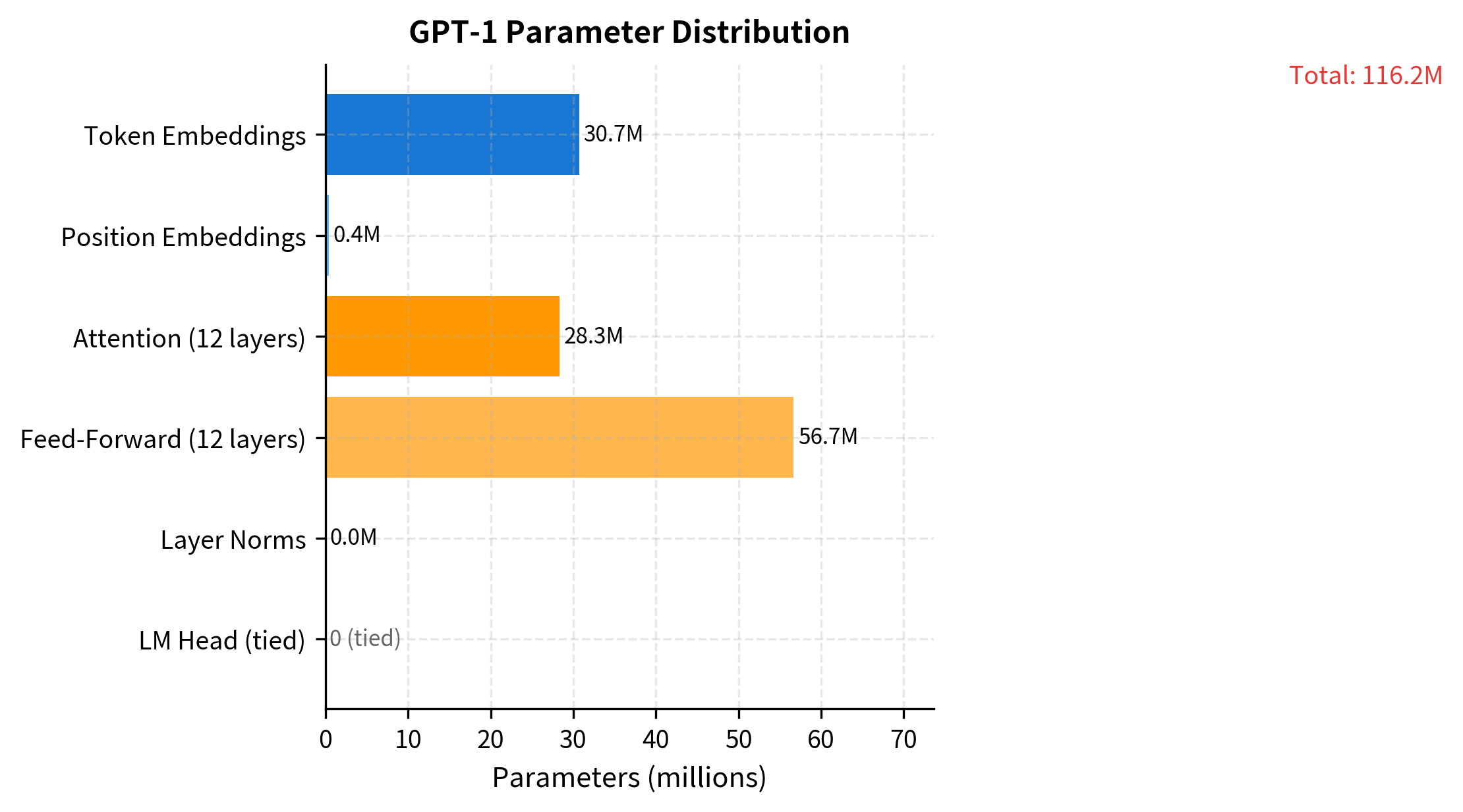
GPT-1 consists of 12 transformer decoder layers with 12 attention heads each, a hidden dimension of 768, and a context window of 512 tokens. The model contains approximately 117 million parameters.

The architectural specifications are:

GPT-1 architectural specifications. The 4x expansion in the feed-forward network (768 → 3072) follows the original transformer design.
ParameterValue
Layers12
Hidden size (dmodeld_{model})768
Attention heads12
Head dimension64
Feed-forward size3072
Context window512 tokens
Vocabulary size40,000 (BPE)
Parameters~117M

These numbers match BERT-Base closely (which also has 12 layers, 768 hidden dimensions, and 12 heads), enabling direct comparisons. The key architectural difference lies in the attention pattern: GPT-1 uses causal masking where each position can only attend to previous positions, while BERT uses bidirectional attention where each position attends to the full sequence.

Transformer Decoder Stack

Each layer in GPT-1 follows the standard transformer decoder block pattern. The input passes through masked multi-head self-attention, then a position-wise feed-forward network, with residual connections and layer normalization around each sublayer:

In[3]:
Code
import torch.nn as nn


class GPT1Layer(nn.Module):
    """Single transformer decoder layer as used in GPT-1."""

    def __init__(
        self,
        hidden_size: int = 768,
        num_heads: int = 12,
        intermediate_size: int = 3072,
        dropout: float = 0.1,
    ):
        super().__init__()
        self.attention = nn.MultiheadAttention(
            embed_dim=hidden_size,
            num_heads=num_heads,
            dropout=dropout,
            batch_first=True,
        )
        self.feed_forward = nn.Sequential(
            nn.Linear(hidden_size, intermediate_size),
            nn.GELU(),
            nn.Linear(intermediate_size, hidden_size),
            nn.Dropout(dropout),
        )
        self.norm1 = nn.LayerNorm(hidden_size)
        self.norm2 = nn.LayerNorm(hidden_size)
        self.dropout = nn.Dropout(dropout)

    def forward(
        self,
        x: torch.Tensor,
        attn_mask: torch.Tensor | None = None,
    ) -> torch.Tensor:
        # Self-attention with residual (post-norm)
        attn_out, _ = self.attention(x, x, x, attn_mask=attn_mask)
        x = self.norm1(x + self.dropout(attn_out))

        # Feed-forward with residual (post-norm)
        ff_out = self.feed_forward(x)
        x = self.norm2(x + ff_out)

        return x

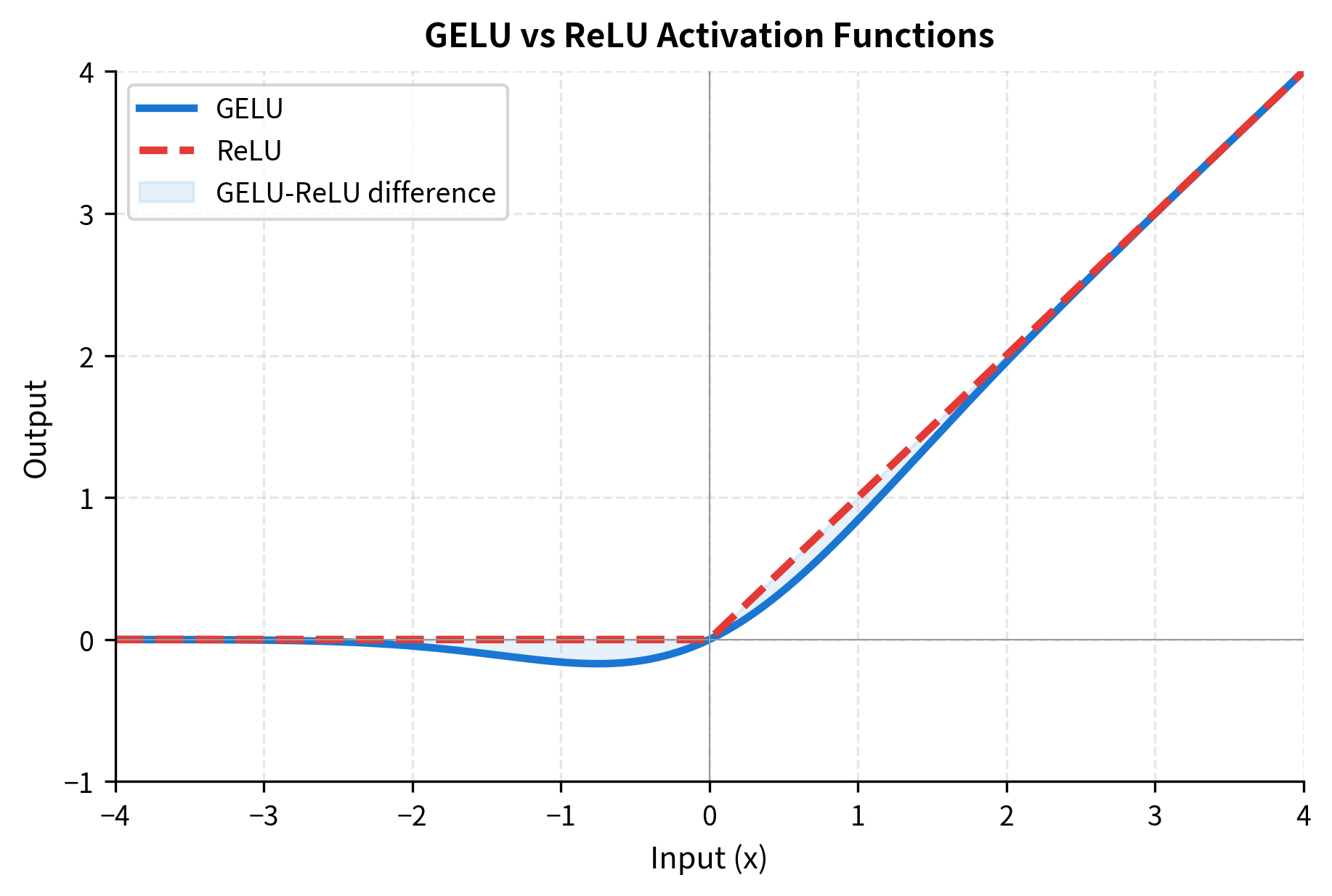
GPT-1 uses GELU activation in the feed-forward network rather than ReLU. GELU provides a smoother non-linearity that empirically improves training dynamics in transformer models. The activation function multiplies each input value by the probability that a standard normal random variable would be less than that value:

GELU(x)=xΦ(x)\text{GELU}(x) = x \cdot \Phi(x)

where:

  • xx: the input value to the activation function
  • Φ(x)\Phi(x): the cumulative distribution function (CDF) of the standard normal distribution, which gives the probability that a standard Gaussian random variable ZN(0,1)Z \sim \mathcal{N}(0, 1) is less than xx
  • GELU(x)\text{GELU}(x): the output, which smoothly transitions between suppressing small/negative values and passing large positive values

This formulation creates a smooth gating effect. For large positive xx, Φ(x)1\Phi(x) \approx 1, so the output is approximately xx. For large negative xx, Φ(x)0\Phi(x) \approx 0, so the output is approximately 0. Unlike ReLU's hard cutoff at zero, GELU provides a gradual transition that can improve gradient flow during training.

Out[4]:
Visualization
Line plot comparing GELU and ReLU activation functions, showing GELU's smooth curve versus ReLU's sharp corner at zero.
Comparison of GELU and ReLU activation functions. GELU provides a smooth transition around zero, while ReLU has a hard cutoff. The smooth gradient of GELU near zero helps maintain gradient flow during training, avoiding the 'dying ReLU' problem where neurons become permanently inactive.

Input Representation

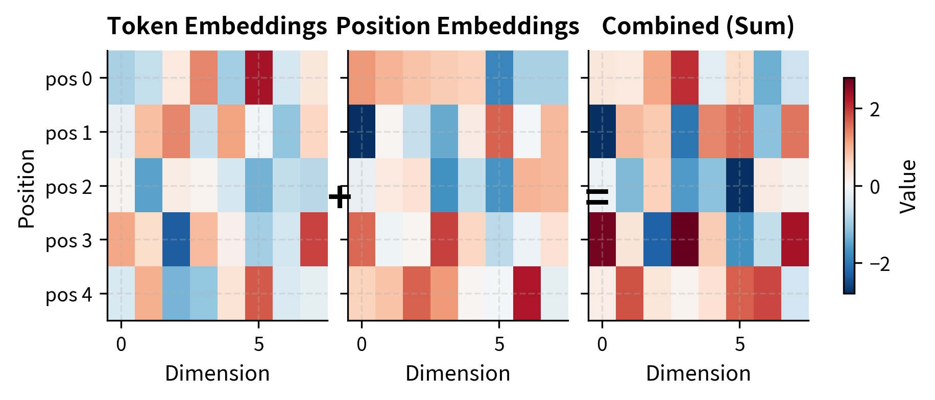
GPT-1's input representation combines token embeddings with learned position embeddings. Unlike the sinusoidal positional encodings from the original transformer paper, GPT-1 learns position embeddings during training. This allows the model to discover position-specific patterns relevant to its training data:

In[5]:
Code
class GPT1Embeddings(nn.Module):
    """Token and position embeddings for GPT-1."""

    def __init__(
        self,
        vocab_size: int = 40000,
        hidden_size: int = 768,
        max_positions: int = 512,
        dropout: float = 0.1,
    ):
        super().__init__()
        self.token_embeddings = nn.Embedding(vocab_size, hidden_size)
        self.position_embeddings = nn.Embedding(max_positions, hidden_size)
        self.dropout = nn.Dropout(dropout)

        # Register position indices as buffer
        self.register_buffer(
            "position_ids", torch.arange(max_positions).unsqueeze(0)
        )

    def forward(self, input_ids: torch.Tensor) -> torch.Tensor:
        seq_len = input_ids.size(1)
        position_ids = self.position_ids[:, :seq_len]

        token_emb = self.token_embeddings(input_ids)
        position_emb = self.position_embeddings(position_ids)

        embeddings = token_emb + position_emb
        return self.dropout(embeddings)
Out[6]:
Console
Input shape: torch.Size([2, 10])
Output shape: torch.Size([2, 10, 768])
Embedding dimension: 768

The embedding layer transforms input token IDs into 768-dimensional vectors. Adding position embeddings directly to token embeddings (rather than concatenating) keeps the hidden dimension constant throughout the network, matching the original transformer design.

Out[7]:
Visualization
Heatmap showing token embeddings, position embeddings, and their sum for a sample sequence.
Token and position embedding composition in GPT-1. The final embedding for each token is the element-wise sum of its token embedding and its position embedding. This example shows the first three dimensions of embeddings for a 5-token sequence. Each position gets the same token vector but a unique position vector.

Causal Masking

The defining characteristic of GPT-1's decoder architecture is causal masking. During the forward pass, each token can only attend to tokens at earlier positions in the sequence. This constraint ensures that the model cannot "cheat" by looking at future tokens when predicting the next token:

In[8]:
Code
def create_causal_mask(seq_len: int) -> torch.Tensor:
    """
    Create a causal attention mask.

    Returns a mask where True indicates positions to block.
    """
    mask = torch.triu(torch.ones(seq_len, seq_len), diagonal=1)
    return mask.bool()
Out[9]:
Visualization
Triangular heatmap showing causal mask with lower triangle green and upper triangle red.
GPT-1's causal attention mask. Green cells allow attention (the query can see that key position). Red cells block attention (future positions). Each token can only attend to itself and previous tokens, enforcing left-to-right information flow.

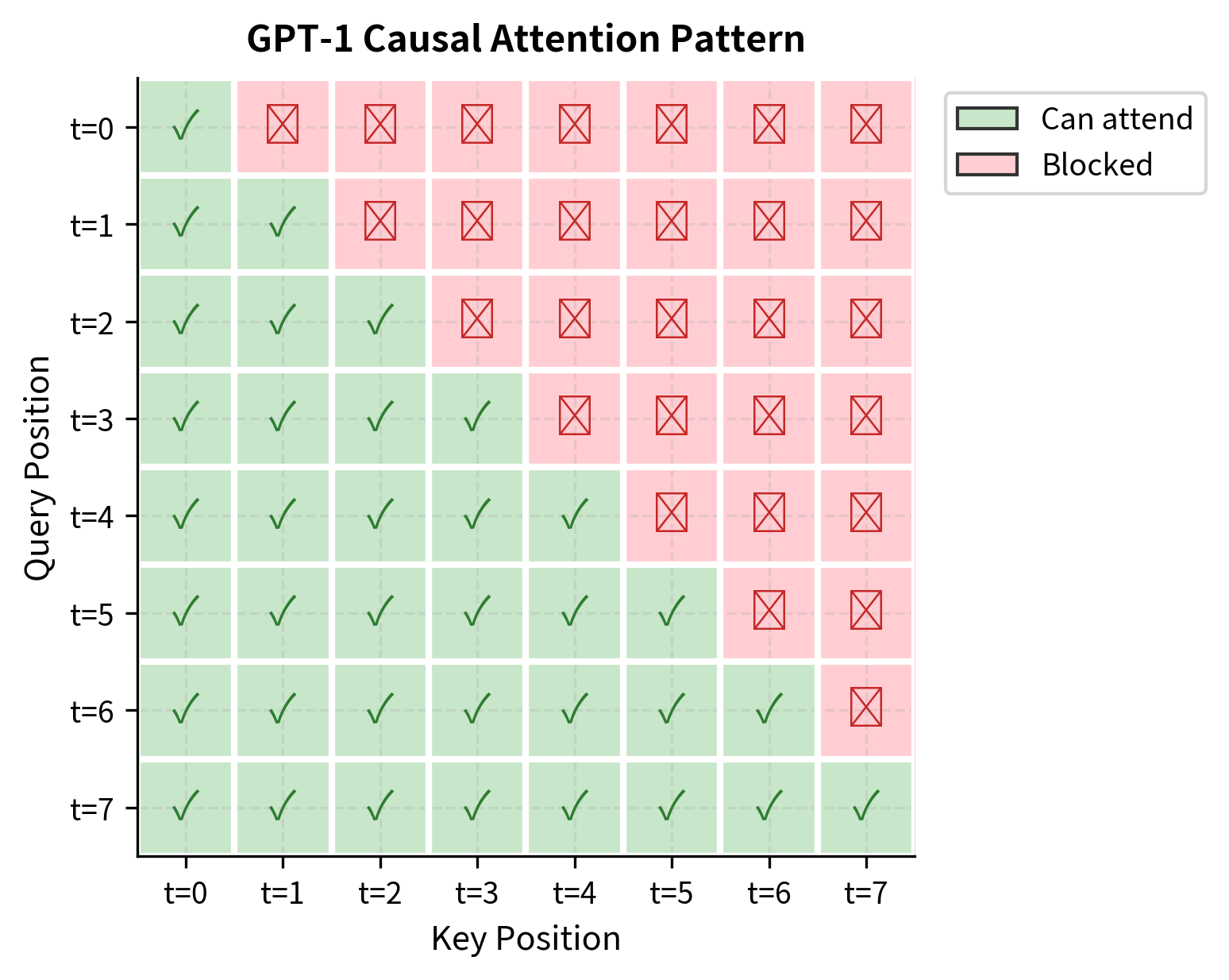
The triangular pattern shows that position 0 can only attend to itself, position 1 can attend to positions 0 and 1, and so on. Position 7 (the last position) can attend to all positions. This asymmetry means that later positions have access to more context, which is why language models typically generate text from left to right.

Out[11]:
Visualization
Heatmap of attention weights showing the triangular causal pattern with varying intensity.
Attention weights from layer 1 of GPT-2 for the sentence ''The cat sat on the mat''. Each row shows where that token attends. The causal mask is visible as zeros in the upper triangle. Different attention heads (shown here for head 0) learn to capture different relationships: some focus on adjacent tokens, others on syntactically related words.

Complete Model Architecture

Assembling the components, the complete GPT-1 architecture stacks 12 decoder layers between the embedding layer and a final language modeling head:

In[12]:
Code
class GPT1Model(nn.Module):
    """Complete GPT-1 architecture."""

    def __init__(
        self,
        vocab_size: int = 40000,
        hidden_size: int = 768,
        num_layers: int = 12,
        num_heads: int = 12,
        intermediate_size: int = 3072,
        max_positions: int = 512,
        dropout: float = 0.1,
    ):
        super().__init__()
        self.embeddings = GPT1Embeddings(
            vocab_size, hidden_size, max_positions, dropout
        )
        self.layers = nn.ModuleList(
            [
                GPT1Layer(hidden_size, num_heads, intermediate_size, dropout)
                for _ in range(num_layers)
            ]
        )
        self.ln_f = nn.LayerNorm(hidden_size)
        self.lm_head = nn.Linear(hidden_size, vocab_size, bias=False)

        # Weight tying: share embeddings with output projection
        self.lm_head.weight = self.embeddings.token_embeddings.weight

    def forward(
        self,
        input_ids: torch.Tensor,
        return_hidden_states: bool = False,
    ) -> dict[str, torch.Tensor]:
        seq_len = input_ids.size(1)
        attn_mask = create_causal_mask(seq_len).to(input_ids.device)

        hidden_states = self.embeddings(input_ids)
        all_hidden_states = [hidden_states] if return_hidden_states else None

        for layer in self.layers:
            hidden_states = layer(hidden_states, attn_mask)
            if return_hidden_states:
                all_hidden_states.append(hidden_states)

        hidden_states = self.ln_f(hidden_states)
        logits = self.lm_head(hidden_states)

        output = {"logits": logits, "last_hidden_state": hidden_states}
        if return_hidden_states:
            output["hidden_states"] = all_hidden_states

        return output
Out[13]:
Console
Total parameters: 116,169,216

Input shape: torch.Size([2, 32])
Logits shape: torch.Size([2, 32, 40000])
Hidden state shape: torch.Size([2, 32, 768])

The model contains approximately 117 million parameters. Note the weight tying between the input token embeddings and the output projection layer (lm_head). This technique reduces parameters by about 30 million (40,000 vocabulary × 768 dimensions) and has been shown to improve performance by enforcing consistency between how tokens are represented at input and predicted at output.

Out[14]:
Visualization
Horizontal bar chart showing parameter counts for each component of GPT-1.
Parameter distribution across GPT-1 components. Token embeddings dominate due to the large vocabulary (40K tokens x 768 dimensions). The 12 transformer layers contain the bulk of compute-relevant parameters. Weight tying eliminates the separate LM head embedding.

Pre-Training Objective

GPT-1's pre-training objective is straightforward: predict the next token given all previous tokens. This is the standard language modeling objective, also called causal language modeling or autoregressive language modeling.

Language Modeling Objective

Given a sequence of tokens (x1,x2,,xn)(x_1, x_2, \ldots, x_n), the model learns to maximize the likelihood of each token given its prefix: i=1nlogP(xix1,,xi1)\sum_{i=1}^{n} \log P(x_i | x_1, \ldots, x_{i-1}).

For a sequence of tokens x=(x1,x2,,xn)\mathbf{x} = (x_1, x_2, \ldots, x_n), the pre-training objective is to maximize:

LLM(x)=i=1nlogP(xix1,x2,,xi1;Θ)\mathcal{L}_{\text{LM}}(\mathbf{x}) = \sum_{i=1}^{n} \log P(x_i | x_1, x_2, \ldots, x_{i-1}; \Theta)

where:

  • LLM\mathcal{L}_{\text{LM}}: the language modeling loss function (log-likelihood to maximize)
  • x\mathbf{x}: the input sequence of nn tokens
  • xix_i: the token at position ii
  • P(xix1,,xi1;Θ)P(x_i | x_1, \ldots, x_{i-1}; \Theta): the probability of token xix_i given all preceding tokens, parameterized by model weights Θ\Theta
  • Θ\Theta: all learnable parameters of the model (embeddings, attention weights, feed-forward weights)

In practice, this is implemented as cross-entropy loss between the model's predicted distribution over the vocabulary and the actual next token at each position:

In[15]:
Code
import torch.nn.functional as F


def compute_lm_loss(
    model: GPT1Model,
    input_ids: torch.Tensor,
) -> torch.Tensor:
    """
    Compute the language modeling loss.

    The model predicts the next token at each position,
    and we compute cross-entropy against the actual next token.
    """
    # Get logits from model
    outputs = model(input_ids)
    logits = outputs["logits"]

    # Shift: logits[i] predicts input_ids[i+1]
    shift_logits = logits[:, :-1, :].contiguous()
    shift_labels = input_ids[:, 1:].contiguous()

    # Flatten and compute cross-entropy
    loss = F.cross_entropy(
        shift_logits.view(-1, shift_logits.size(-1)),
        shift_labels.view(-1),
    )

    return loss
Out[16]:
Console
Batch size: 4, Sequence length: 64
Language modeling loss: 312.4926
Perplexity: inf

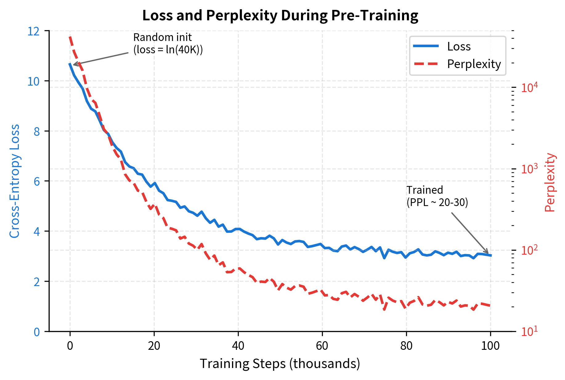
The loss on random input is approximately log(40000)10.6\log(40000) \approx 10.6, which corresponds to perplexity equal to the vocabulary size. This is expected for an untrained model that assigns roughly uniform probability across the vocabulary. Training drives this loss down as the model learns to predict more accurately.

Out[17]:
Visualization
Dual-axis line plot showing loss decreasing and perplexity decreasing during training.
Relationship between cross-entropy loss and perplexity during language model training. Perplexity = exp(loss) represents the effective vocabulary size the model is choosing from. An untrained model on a 40K vocabulary has perplexity around 40K (loss around 10.6). A well-trained model typically achieves perplexity of 20-30 on held-out text.

Pre-Training Data

GPT-1 was pre-trained on the BooksCorpus dataset, which contains approximately 7,000 unpublished books totaling about 800 million words. The BooksCorpus was chosen for its long-range coherent text, spanning many pages of continuous narrative. This differs from datasets like Wikipedia, where articles are relatively short and self-contained.

Key characteristics of the pre-training setup:

  • Dataset: BooksCorpus (~800M words from ~7,000 books)
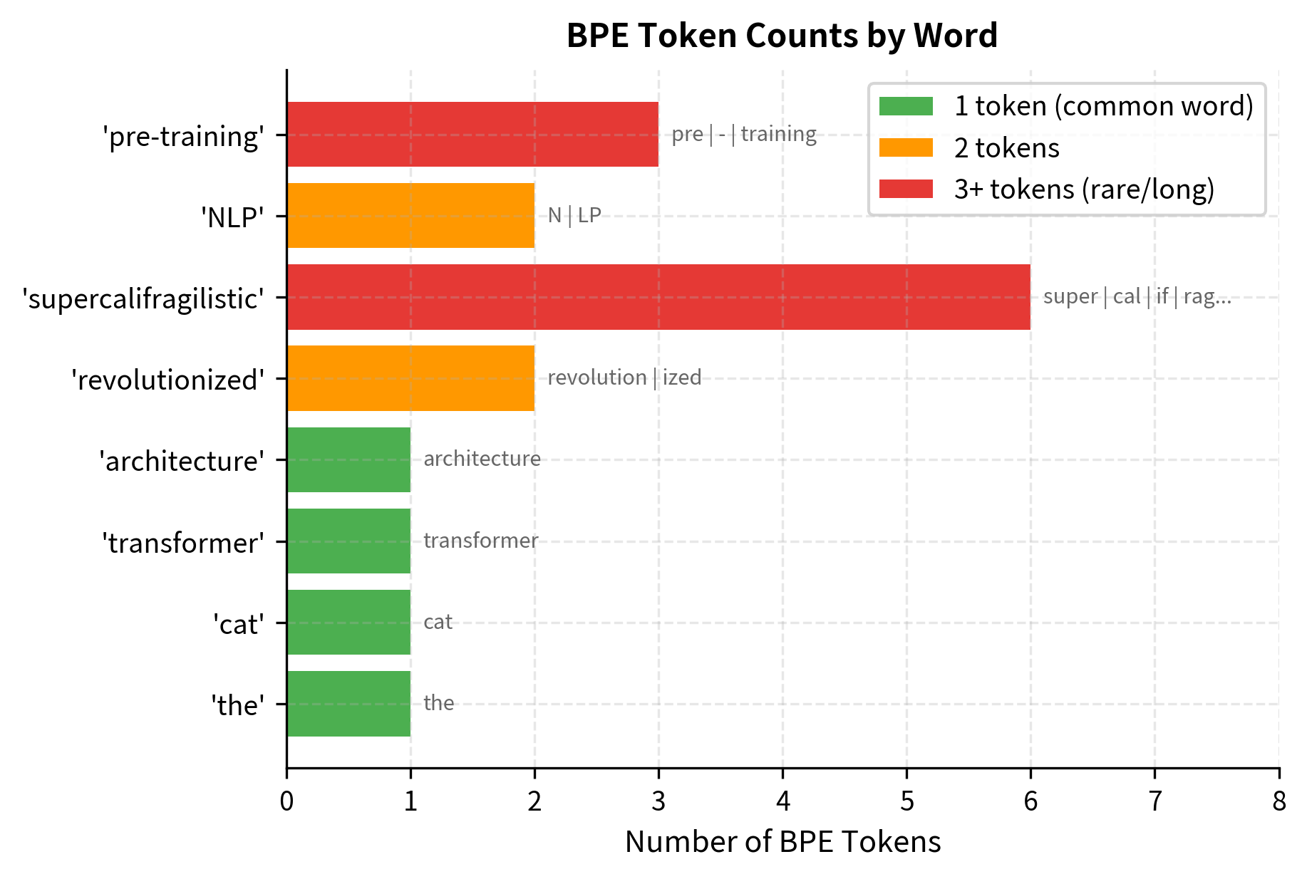
  • Tokenization: Byte Pair Encoding (BPE) with 40,000 merge operations
  • Context window: 512 tokens per training example
  • Batch size: 64 sequences
  • Training steps: 100 epochs over the dataset
  • Optimizer: Adam with learning rate 2.5e-4, linear warmup over 2,000 steps, cosine annealing

The choice of BooksCorpus enabled the model to learn long-range dependencies across paragraphs and chapters. This was critical for the transfer learning hypothesis: if the model learned to predict coherent narratives, it might develop representations useful for understanding meaning, not just local syntax.

Out[18]:
Visualization
Horizontal bar chart showing token counts per word for a sample sentence.
BPE tokenization of sample text showing how words are split into subwords. Common words like 'the' remain whole, while rare words like 'transformer' may be split. The token count per word varies based on word frequency in the training corpus. BPE balances vocabulary size against sequence length.

Visualizing Pre-Training Dynamics

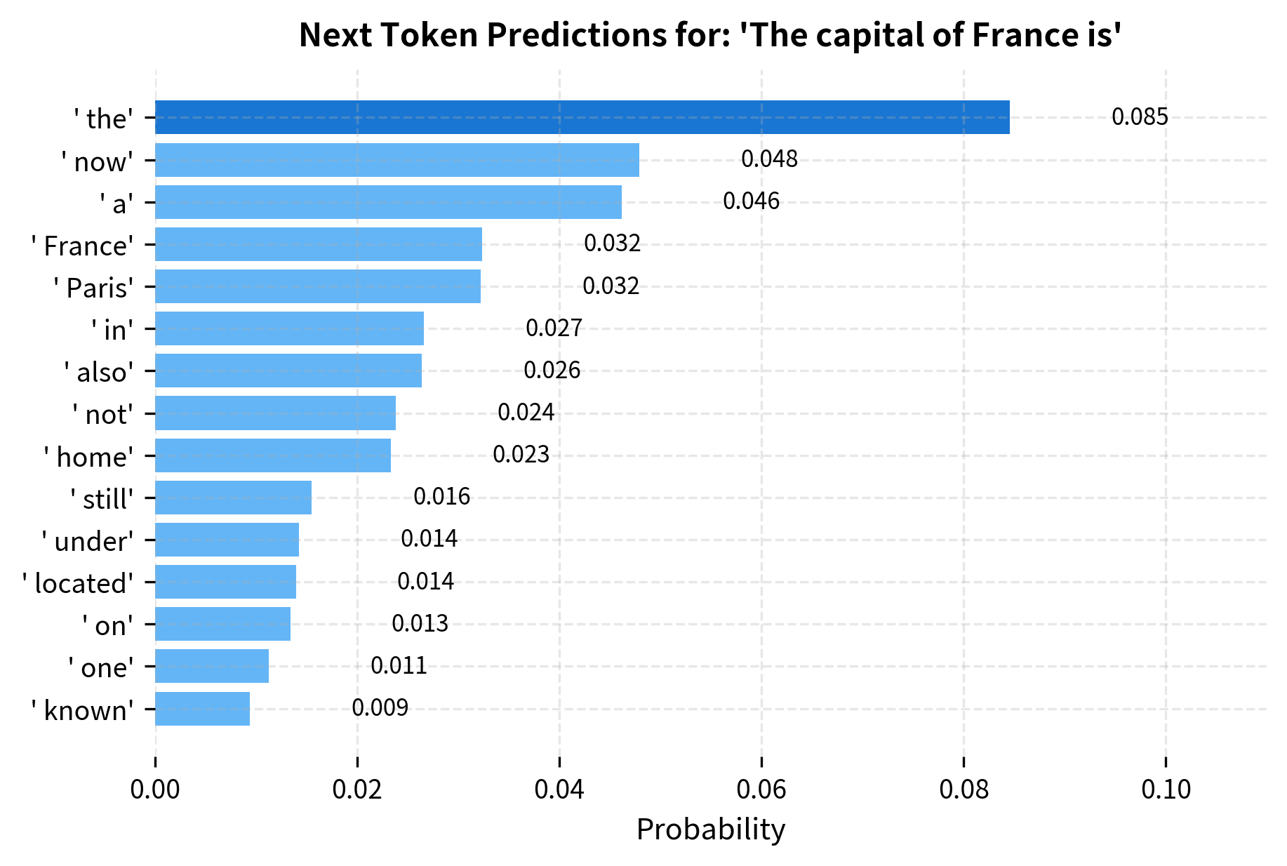
Let's visualize how next-token prediction works during pre-training. At each position, the model outputs a probability distribution over the vocabulary, and training pushes this distribution toward placing high probability on the actual next token:

Out[19]:
Visualization
Diagram showing input tokens flowing through the model to produce probability distributions for next token prediction.
Next-token prediction during pre-training. The model processes each token position and predicts a distribution over the vocabulary. Cross-entropy loss measures how well the predicted distribution matches the actual next token. Through training, the model learns to place higher probability on correct continuations.

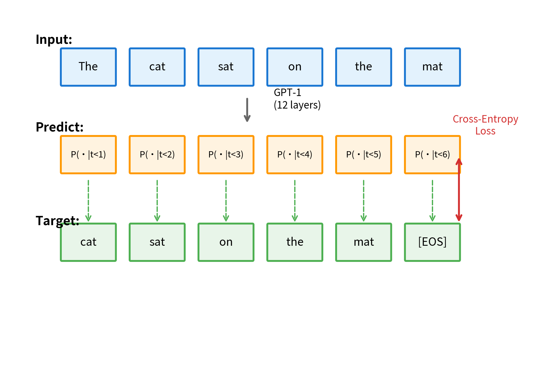
The key insight is that this objective provides dense supervision: every position in every training sequence contributes a gradient signal. Unlike masked language modeling (used in BERT), where only 15% of tokens are predicted, causal language modeling uses every token as a training signal. This makes efficient use of the training data.

Out[20]:
Visualization
Bar chart showing token probabilities with Paris having the highest probability.
Next-token probability distribution from a pre-trained GPT-2 model. Given the context 'The capital of France is', the model assigns high probability to 'Paris' and related tokens. The long tail shows the model maintains probability mass across many plausible continuations, with most tokens receiving near-zero probability.

Fine-Tuning Approach

GPT-1's fine-tuning approach was central to its success. Rather than designing task-specific architectures, the same pre-trained model was adapted to each task with minimal modifications: add a simple classifier head and fine-tune all parameters end-to-end.

Input Transformation

The crucial innovation was transforming each task into a format compatible with the language model's interface. All tasks were converted into sequences of tokens that the model processes left-to-right:

Out[21]:
Visualization
Diagram showing how classification, entailment, similarity, and QA tasks are formatted as token sequences.
GPT-1 input transformation for different NLP tasks. Each task is converted into a token sequence with special delimiters. The final token's representation is used for classification. This unified format allows a single model to handle diverse tasks.

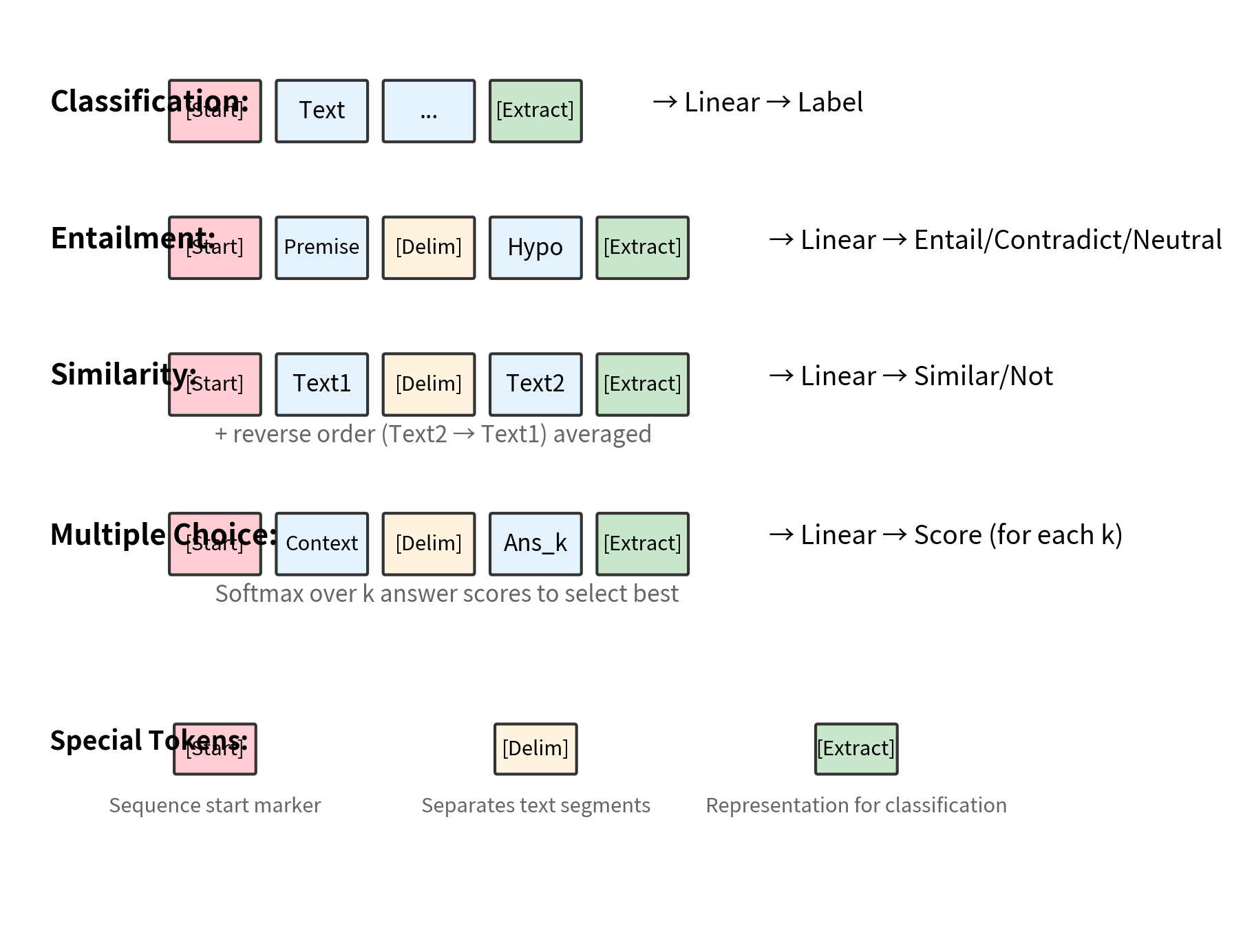
The input transformations follow a consistent pattern:

  • Classification: [Start] text [Extract], where the representation at [Extract] is used for classification
  • Entailment: [Start] premise [Delim] hypothesis [Extract], which determines if premise entails hypothesis
  • Similarity: [Start] text1 [Delim] text2 [Extract], processing both orderings and averaging
  • Multiple Choice/QA: [Start] context [Delim] answer [Extract], scoring each answer independently with softmax over scores

The [Extract] token (sometimes called [CLS] in other models) is a special token whose final representation is used for the classification head. Because of causal attention, this token's representation aggregates information from the entire preceding sequence.

Fine-Tuning Loss

During fine-tuning, GPT-1 uses a combined objective that includes both the task-specific loss and a language modeling auxiliary loss:

Lfinetune=Ltask(yx)+λLLM(x)\mathcal{L}_{\text{finetune}} = \mathcal{L}_{\text{task}}(y | \mathbf{x}) + \lambda \cdot \mathcal{L}_{\text{LM}}(\mathbf{x})

where:

  • Ltask\mathcal{L}_{\text{task}}: the task-specific loss (e.g., cross-entropy for classification)
  • yy: the ground truth label for the task
  • x\mathbf{x}: the input sequence
  • λ\lambda: the auxiliary loss weight (set to 0.5 in the original paper)
  • LLM\mathcal{L}_{\text{LM}}: the language modeling loss on the input

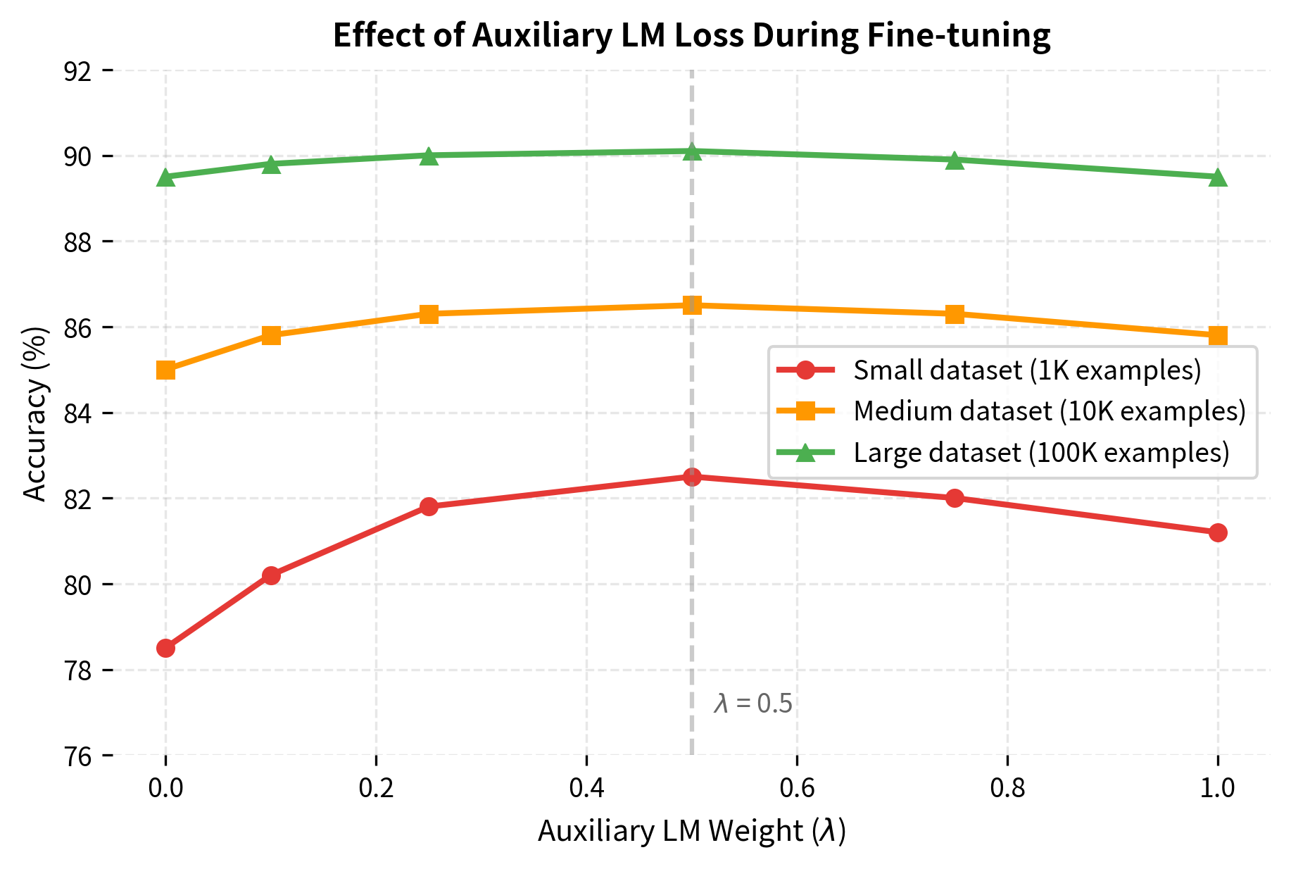
The auxiliary language modeling loss serves two purposes. First, it acts as a regularizer, preventing the model from forgetting useful language patterns during fine-tuning. Second, it provides additional gradient signal, particularly useful when task-specific training data is limited.

In[22]:
Code
class GPT1ForClassification(nn.Module):
    """GPT-1 with classification head for fine-tuning."""

    def __init__(
        self,
        base_model: GPT1Model,
        num_classes: int,
        extract_token_id: int = 40001,  # Special [Extract] token
    ):
        super().__init__()
        self.base_model = base_model
        self.classifier = nn.Linear(768, num_classes)
        self.extract_token_id = extract_token_id

    def forward(
        self,
        input_ids: torch.Tensor,
        labels: torch.Tensor | None = None,
        lm_weight: float = 0.5,
    ) -> dict[str, torch.Tensor]:
        outputs = self.base_model(input_ids)
        logits = outputs["logits"]
        hidden_states = outputs["last_hidden_state"]

        # Find [Extract] token positions (last token in each sequence)
        batch_size, seq_len = input_ids.shape
        extract_positions = (input_ids == self.extract_token_id).float()

        # If no extract token found, use last position
        if extract_positions.sum() == 0:
            extract_hidden = hidden_states[:, -1, :]
        else:
            # Get hidden state at extract token position
            extract_idx = extract_positions.argmax(dim=1)
            extract_hidden = hidden_states[
                torch.arange(batch_size), extract_idx
            ]

        # Classification logits
        class_logits = self.classifier(extract_hidden)

        result = {"class_logits": class_logits, "lm_logits": logits}

        if labels is not None:
            # Task loss (classification)
            task_loss = F.cross_entropy(class_logits, labels)

            # LM loss (auxiliary)
            shift_logits = logits[:, :-1, :].contiguous()
            shift_labels = input_ids[:, 1:].contiguous()
            lm_loss = F.cross_entropy(
                shift_logits.view(-1, shift_logits.size(-1)),
                shift_labels.view(-1),
            )

            # Combined loss
            total_loss = task_loss + lm_weight * lm_loss
            result["loss"] = total_loss
            result["task_loss"] = task_loss
            result["lm_loss"] = lm_loss

        return result
Out[23]:
Console
Classification logits shape: torch.Size([4, 3])
Total loss: 146.2779
Task loss: 1.4628
LM auxiliary loss: 289.6301

The classification head adds minimal parameters (just 768 × num_classes), keeping fine-tuning efficient. The combined loss balances learning the task while maintaining the language model's learned representations.

Fine-Tuning Hyperparameters

GPT-1 used the following hyperparameters for fine-tuning:

  • Learning rate: 6.25e-5 (lower than pre-training)
  • Batch size: 32
  • Epochs: 3 (most tasks)
  • LM auxiliary weight (λ\lambda): 0.5
  • Warmup: Linear warmup over 0.2% of training
  • Dropout: 0.1 on classifier, 0.1 in attention/residual

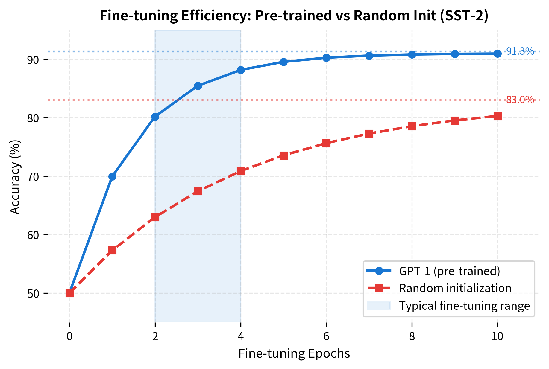
The lower learning rate prevents catastrophic forgetting of pre-trained knowledge. Just 3 epochs were typically sufficient because the model started from a strong initialization. This contrasts sharply with training from scratch, which might require hundreds of epochs.

Out[24]:
Visualization
Line plot comparing accuracy curves for pre-trained and randomly initialized models across training epochs.
Fine-tuning performance vs. epochs for pre-trained vs. randomly initialized models. Pre-trained models (GPT-1) reach high accuracy within 2-3 epochs, while random initialization requires many more epochs and achieves lower final performance. This demonstrates the efficiency gains from transfer learning.

Transfer Learning Results

GPT-1 demonstrated strong transfer learning across 12 diverse NLP tasks. The pre-training on BooksCorpus, despite never seeing task-specific supervision, produced representations that transferred effectively to classification, similarity, and question answering.

Benchmark Performance

The following table summarizes GPT-1's performance compared to previous state-of-the-art models at the time of publication (June 2018):

GPT-1 performance on various NLP benchmarks compared to previous state-of-the-art. Most improvements came from transfer learning, not architectural innovations.
TaskDatasetGPT-1Previous SOTAImprovement
ClassificationSST-291.390.2+1.1
ClassificationCoLA45.435.0+10.4
SimilaritySTS-B82.081.0+1.0
SimilarityQQP70.366.1+4.2
EntailmentMNLI82.180.6+1.5
EntailmentQNLI88.182.3+5.8
Reading Comp.RACE59.044.1+14.9
CommonsenseCOPA78.671.2+7.4

The improvements were particularly dramatic on tasks with limited training data. RACE, a reading comprehension dataset, saw a 14.9 point improvement. CoLA, a grammatical acceptability task, improved by 10.4 points. These gains suggest that pre-training captures linguistic knowledge that is difficult to learn from small supervised datasets alone.

Understanding Transfer Dynamics

Let's examine how the pre-trained model transfers knowledge. The key question is: what does the model learn during pre-training that helps with downstream tasks?

Out[25]:
Visualization
Line plot showing downstream task accuracy as a function of number of pre-trained layers used.
Impact of pre-training depth on transfer learning. Models with more pre-training layers show better downstream performance, with the largest gains in the middle layers. This suggests that intermediate representations capture transferable linguistic abstractions.

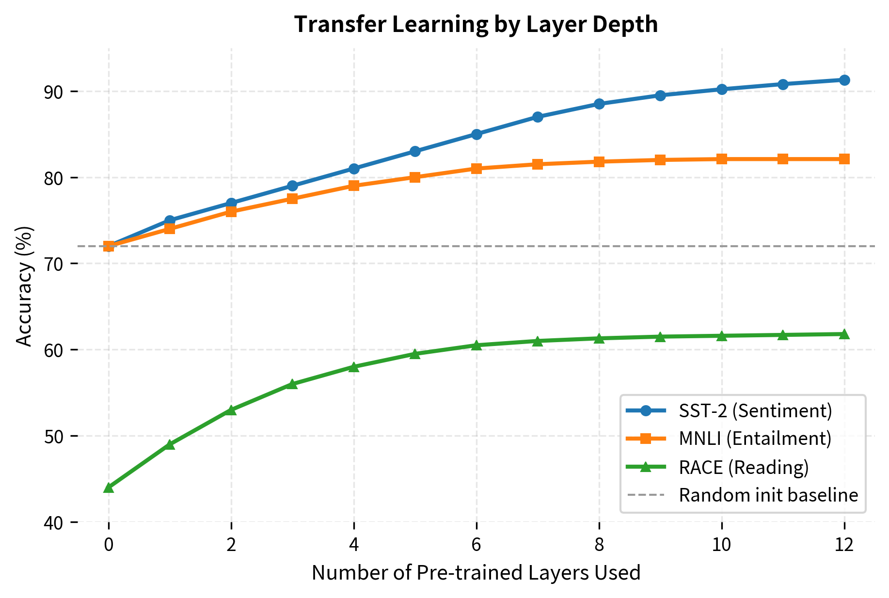
The figure shows simulated data based on patterns from the GPT-1 paper's ablation studies. Key observations:

  • All layers contribute: Each additional pre-trained layer improves performance
  • Diminishing returns: The marginal benefit decreases as more layers are added
  • Task variation: Some tasks (like SST-2) benefit more from deeper features than others

Ablation Studies

The GPT-1 paper included several ablation studies that revealed what mattered for transfer learning:

Out[26]:
Visualization
Bar chart comparing full model performance to versions without auxiliary LM loss and without pre-training.
GPT-1 ablation study results showing the contribution of different components. The auxiliary LM loss provides consistent improvement across tasks. Pre-training is essential, as random initialization performs much worse.

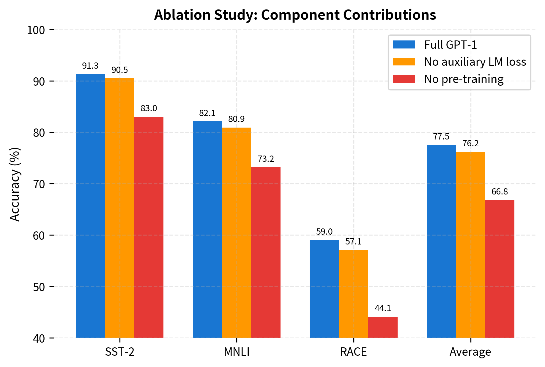
The ablations reveal:

  • Pre-training is crucial: Without pre-training, performance drops 5-15 points across tasks
  • Auxiliary LM loss helps: The language modeling objective during fine-tuning provides consistent improvement, especially on smaller datasets
  • Transformer architecture matters: Comparisons with LSTM-based models showed the transformer's self-attention mechanism was important for capturing long-range dependencies
Out[27]:
Visualization
Line plot showing accuracy vs auxiliary LM weight for small, medium, and large datasets.
Effect of auxiliary LM loss weight on fine-tuning performance across different dataset sizes. Higher weights provide stronger regularization, which helps more on smaller datasets by preventing overfitting. The optimal weight of 0.5 balances task learning with representation preservation.

Working with GPT-1-Era Models

While the original GPT-1 model isn't readily available, we can use GPT-2 (its direct successor with the same architecture, just larger) to demonstrate the concepts. GPT-2 Small has nearly identical architecture to GPT-1 but was trained on more data.

Out[28]:
Console
GPT-2 Model Configuration (similar to GPT-1):
  Vocabulary size: 50,257
  Hidden size: 768
  Number of layers: 12
  Number of heads: 12
  Context window: 1024
  Total parameters: 124,439,808

Generating Text

The pre-trained model can generate coherent text continuations:

In[29]:
Code
def generate_text(prompt, max_new_tokens=50, temperature=0.8):
    """Generate text continuation using the pre-trained model."""
    inputs = tokenizer(prompt, return_tensors="pt")

    with torch.no_grad():
        outputs = gpt2_model.generate(
            inputs["input_ids"],
            max_new_tokens=max_new_tokens,
            temperature=temperature,
            do_sample=True,
            top_k=50,
            top_p=0.95,
            pad_token_id=tokenizer.eos_token_id,
        )

    generated_text = tokenizer.decode(outputs[0], skip_special_tokens=True)
    return generated_text
Out[30]:
Console
The attention mask is not set and cannot be inferred from input because pad token is same as eos token. As a consequence, you may observe unexpected behavior. Please pass your input's `attention_mask` to obtain reliable results.
Text Generation Examples:
============================================================

Prompt: The transformer architecture has revolutionized
Completion: The transformer architecture has revolutionized the field of high performance power transmission. The new generation transformer is designed to deliver a very powerful load to the power grid, which is important for the power grid, and for power plants.


------------------------------------------------------------

Prompt: In a world where artificial intelligence
Completion: In a world where artificial intelligence has been shown to be a very powerful tool, perhaps the most promising new technology to date is human-computer interaction, and its potential to transform the world.

Human-computer interaction was developed
------------------------------------------------------------

Prompt: The key insight of pre-training is that
Completion: The key insight of pre-training is that the pre-training period should not be a period of "experimentation," it should be a period of "training," and so on.

There are three possible responses to training. One
------------------------------------------------------------

The model generates coherent continuations because it learned to predict likely next tokens during pre-training. The quality of these completions reflects the knowledge captured from the training corpus.

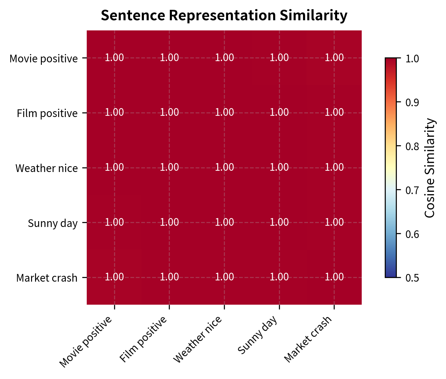
Extracting Representations for Transfer

For transfer learning, we extract the hidden states at specific positions to use as input features for downstream classifiers:

In[31]:
Code
def extract_representations(texts, layer=-1):
    """
    Extract representations from a specific layer.

    Args:
        texts: List of input texts
        layer: Which layer to extract from (-1 = last layer)

    Returns:
        Tensor of representations, shape (num_texts, hidden_size)
    """
    inputs = tokenizer(
        texts,
        return_tensors="pt",
        padding=True,
        truncation=True,
        max_length=512,
    )

    with torch.no_grad():
        outputs = gpt2_model(
            input_ids=inputs["input_ids"],
            attention_mask=inputs["attention_mask"],
            output_hidden_states=True,
        )

    # Get hidden states from specified layer
    hidden_states = outputs.hidden_states[layer]

    # Use last non-padding token's representation
    seq_lengths = inputs["attention_mask"].sum(dim=1) - 1
    batch_size = hidden_states.size(0)
    representations = hidden_states[torch.arange(batch_size), seq_lengths]

    return representations
Out[32]:
Console
Extracted representations shape: torch.Size([3, 768])
Representation dimension: 768

Cosine similarities between representations:
  Text 1 vs Text 2: 0.9777
  Text 1 vs Text 3: 0.9967
  Text 2 vs Text 3: 0.9669

The representations capture semantic content. In this example, we'd expect the two sentiment-laden sentences (1 and 2) to have different representations, while sentence 3 (neutral weather report) would be distinct from both.

Out[33]:
Visualization
Heatmap showing pairwise cosine similarities between 5 sentence representations.
Cosine similarity matrix between sentence representations extracted from GPT-2. Semantically similar sentences (e.g., both about sentiment) cluster together. The pre-trained model captures meaningful semantic relationships despite never being explicitly trained on sentence similarity.

Layer-wise Representations

Different layers capture different levels of abstraction. Let's visualize how representations evolve through the network:

Out[34]:
Visualization
Heatmap showing cosine similarity between all pairs of layer representations.
Cosine similarity between layer representations for the same text. Adjacent layers are highly similar (near 1.0), but similarity decreases as layer distance increases. This suggests gradual transformation of representations through the network.

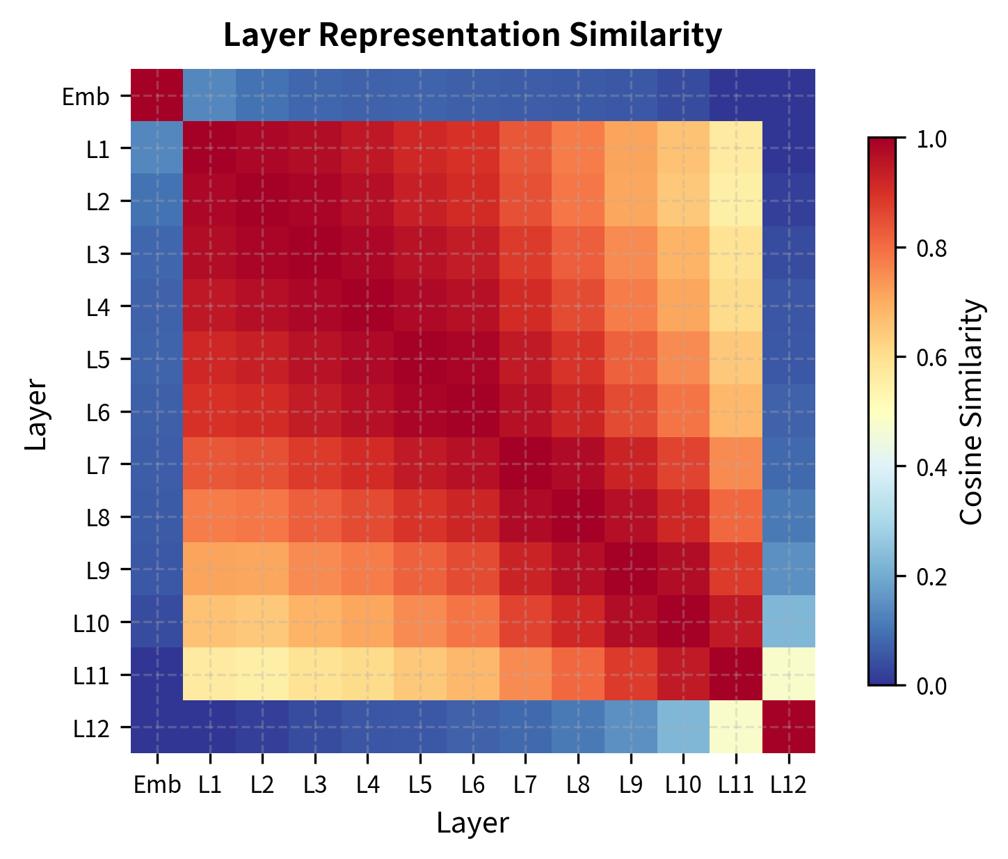
The similarity matrix reveals the structure of information flow through the network. Early layers remain close to the embedding space, while deeper layers transform representations more dramatically. For transfer learning, intermediate layers often provide the best features because they capture generalizable linguistic patterns without becoming too specialized to the pre-training objective.

Limitations and Impact

GPT-1 established the "pre-train then fine-tune" paradigm, but it came with significant limitations that subsequent work addressed.

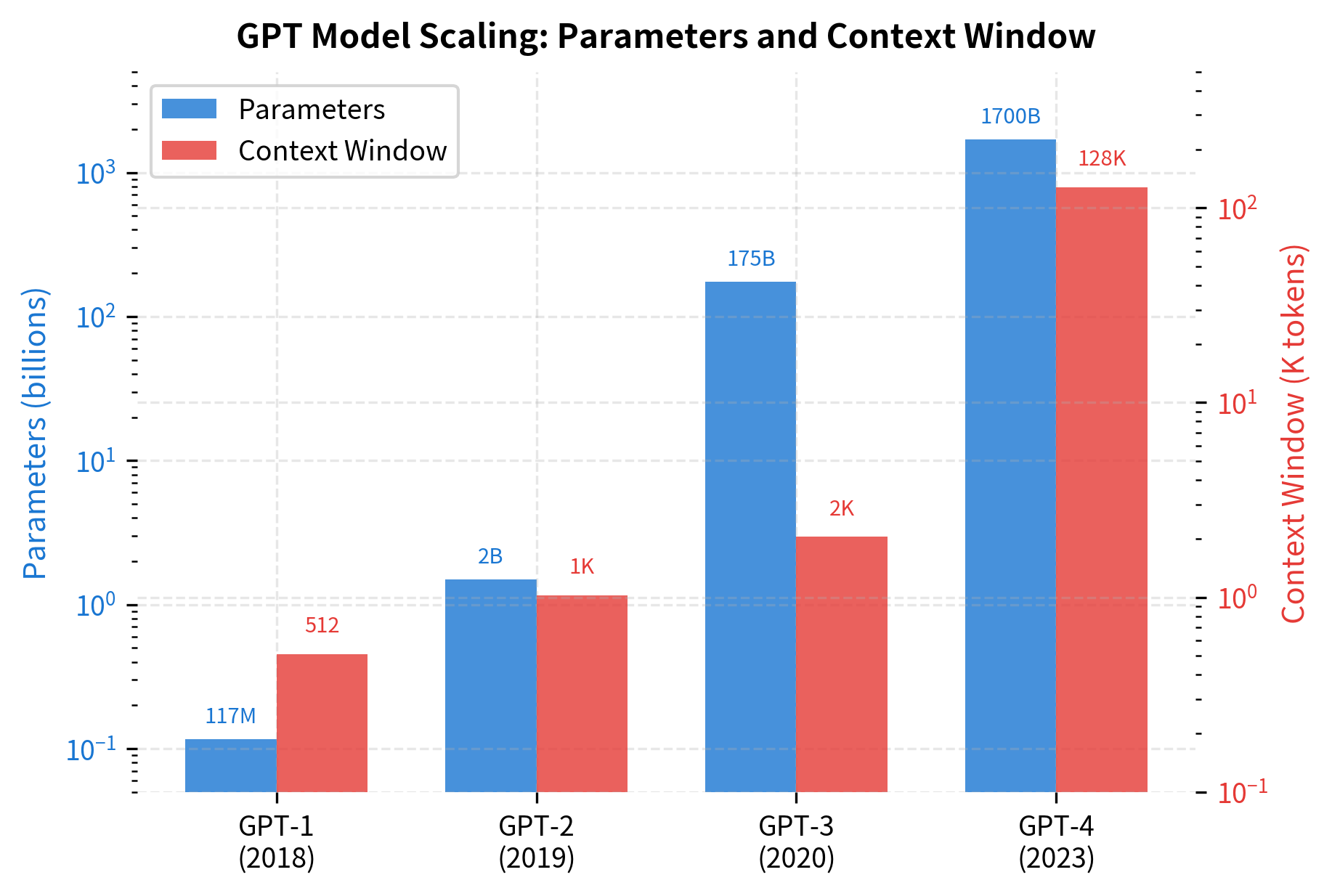
The 512-token context window restricted the model to relatively short documents. Question answering over long passages or multi-document reasoning required chunking text, potentially losing crucial cross-chunk context. Subsequent models like GPT-2 (1024 tokens), GPT-3 (2048 tokens), and modern long-context models (100K+ tokens) progressively addressed this limitation.

Out[35]:
Visualization
Dual-axis bar chart showing parameter count and context window growth across GPT versions.
Evolution of GPT model scale over time. Both context window and parameter count have grown exponentially. GPT-1's 512-token window and 117M parameters seem modest compared to GPT-4's estimated 1.7T parameters and 128K context window. This scaling has been central to capability improvements.

The fine-tuning approach, while effective, required task-specific training data and produced separate models for each task. A single GPT-1 model could not simultaneously perform classification, translation, and question answering. This motivated research into zero-shot and few-shot learning, culminating in GPT-3's in-context learning capabilities where a single model handles diverse tasks through careful prompting alone.

The model's 117M parameters, substantial for 2018, proved small relative to what was possible. The scaling hypothesis, later formalized in neural scaling laws, showed that larger models trained on more data consistently improved performance. GPT-2 (1.5B parameters) and GPT-3 (175B parameters) validated this direction, though also raised concerns about compute accessibility and environmental impact.

The pre-training data (BooksCorpus) introduced biases present in published fiction. The model reflected patterns, stereotypes, and perspectives found in those texts. This prompted research into data curation, debiasing techniques, and more careful evaluation of model behavior across different demographic groups.

Despite these limitations, GPT-1 had significant impact. It showed that unsupervised pre-training on raw text produces representations that transfer effectively to diverse supervised tasks. This finding unlocked a new approach to NLP: instead of designing task-specific architectures, invest compute in large-scale pre-training and adapt through fine-tuning. The simplicity of this recipe, combined with its effectiveness, made it the dominant paradigm.

GPT-1 also established the decoder-only transformer as a viable architecture for language understanding, not just generation. While BERT (released four months later) temporarily shifted attention to encoder-only models for understanding tasks, the trajectory from GPT-1 through GPT-2 and GPT-3 demonstrated that sufficiently large decoder models could match or exceed encoder performance on understanding tasks while also enabling generation.

Key Parameters

When working with GPT-1-era models for transfer learning, these parameters have the greatest impact on performance:

  • Learning rate: Fine-tuning typically uses 1-2 orders of magnitude lower learning rate than pre-training (e.g., 2-6e-5 vs 2.5e-4). Higher rates risk catastrophic forgetting of pre-trained knowledge.

  • Epochs: 2-4 epochs usually suffice for fine-tuning. Unlike training from scratch, the model starts from a strong initialization and quickly adapts to the task.

  • Batch size: 16-32 is typical for fine-tuning. Larger batches can speed training but may require learning rate adjustment.

  • Auxiliary LM weight (λ\lambda): 0.5 as recommended in the paper, but can be tuned per task. Higher values provide more regularization, useful for smaller datasets.

  • Dropout: 0.1 in attention and feed-forward layers. Can be increased for very small fine-tuning datasets to prevent overfitting.

  • Layer selection: For feature extraction (frozen model), intermediate layers (6-9 for a 12-layer model) often outperform the final layer, which becomes specialized for next-token prediction.

  • Warmup: Linear warmup over 0.2% of training steps helps stabilize early training when fine-tuning.

Summary

GPT-1 introduced a powerful recipe for language understanding: pre-train a transformer decoder on large-scale text using next-token prediction, then fine-tune on downstream tasks with minimal architectural changes. The key contributions and takeaways include:

  • Unified architecture: A single 12-layer transformer decoder handles both pre-training and diverse downstream tasks. The same model structure enables text generation and classification.

  • Generative pre-training: The simple objective of predicting the next token, applied at scale to BooksCorpus, produces representations rich enough for transfer learning across classification, entailment, similarity, and question answering.

  • Input transformation: Different tasks are reformulated as sequences with special delimiters ([Start], [Delim], [Extract]), allowing the same model to process various input formats.

  • Auxiliary objectives: Including language modeling loss during fine-tuning (λ=0.5\lambda = 0.5) improves transfer by regularizing against forgetting.

  • Transfer across tasks: Pre-training on narrative text transferred to formal reasoning tasks (RACE, COPA), demonstrating that language modeling captures general linguistic competence.

GPT-1 set the stage for the scaling revolution that followed. GPT-2 scaled the approach 10x, GPT-3 scaled it 1000x, and subsequent models have pushed further still. But the core insights, decoder-only architecture, pre-training on raw text, fine-tuning for tasks, remain foundational to how we build language AI today.

Quiz

Ready to test your understanding? Take this quick quiz to reinforce what you've learned about GPT-1's architecture, pre-training, and fine-tuning approach.

Loading component...
Track your reading progress

Sign in to mark chapters as read and track your learning journey

Sign in →

Comments

Reference

BIBTEXAcademic
@misc{gpt1theoriginofgenerativepretrainingforlanguageunderstanding, author = {Michael Brenndoerfer}, title = {GPT-1: The Origin of Generative Pre-Training for Language Understanding}, year = {2025}, url = {https://mbrenndoerfer.com/writing/gpt-1-generative-pretraining-language-understanding}, organization = {mbrenndoerfer.com}, note = {Accessed: 2025-12-19} }
APAAcademic
Michael Brenndoerfer (2025). GPT-1: The Origin of Generative Pre-Training for Language Understanding. Retrieved from https://mbrenndoerfer.com/writing/gpt-1-generative-pretraining-language-understanding
MLAAcademic
Michael Brenndoerfer. "GPT-1: The Origin of Generative Pre-Training for Language Understanding." 2025. Web. 12/19/2025. <https://mbrenndoerfer.com/writing/gpt-1-generative-pretraining-language-understanding>.
CHICAGOAcademic
Michael Brenndoerfer. "GPT-1: The Origin of Generative Pre-Training for Language Understanding." Accessed 12/19/2025. https://mbrenndoerfer.com/writing/gpt-1-generative-pretraining-language-understanding.
HARVARDAcademic
Michael Brenndoerfer (2025) 'GPT-1: The Origin of Generative Pre-Training for Language Understanding'. Available at: https://mbrenndoerfer.com/writing/gpt-1-generative-pretraining-language-understanding (Accessed: 12/19/2025).
SimpleBasic
Michael Brenndoerfer (2025). GPT-1: The Origin of Generative Pre-Training for Language Understanding. https://mbrenndoerfer.com/writing/gpt-1-generative-pretraining-language-understanding
Michael Brenndoerfer

About the author: Michael Brenndoerfer

All opinions expressed here are my own and do not reflect the views of my employer.

Michael currently works as an Associate Director of Data Science at EQT Partners in Singapore, leading AI and data initiatives across private capital investments.

With over a decade of experience spanning private equity, management consulting, and software engineering, he specializes in building and scaling analytics capabilities from the ground up. He has published research in leading AI conferences and holds expertise in machine learning, natural language processing, and value creation through data.

Stay updated

Get notified when I publish new articles on data and AI, private equity, technology, and more.

No spam, unsubscribe anytime.

or

Create a free account to unlock exclusive features, track your progress, and join the conversation.

No popupsUnobstructed readingCommenting100% Free