Rotary Position Embedding (RoPE): Encoding Position Through Rotation

The transformer attention mechanism, as we've seen, is inherently position-blind. Sinusoidal encodings and learned position embeddings address this by adding position information to token embeddings before attention. But these approaches encode absolute position. Token at position 5 always receives the same positional signal, regardless of context. What if the relationship between positions 5 and 7 matters more than the absolute locations? Relative position encoding tackles this, but earlier methods required modifying the attention architecture or adding explicit bias terms.

Rotary Position Embedding, or RoPE, takes an elegant geometric approach. Instead of adding position to embeddings, it rotates them. Each position corresponds to a rotation angle, and the rotation is applied directly to query and key vectors. The ingenious part: when you compute the dot product between a rotated query at position $m$ and a rotated key at position $n$, the result depends only on their relative distance $m - n$. Absolute positions vanish, leaving only the relationship between tokens.

This chapter develops RoPE from first principles. We'll start with rotations in 2D, extend to higher dimensions through paired rotations, derive why the mechanism captures relative position, and implement it in code. By the end, you'll understand why RoPE has become the dominant position encoding in modern language models like LLaMA, PaLM, and many others.

Consider what we want from a position encoding. When a query at position $m$ attends to a key at position $n$, the attention score should somehow reflect their relative distance $m - n$. If token 3 attends to token 1, the model should "know" they're 2 positions apart, exactly as if token 8 attends to token 6.

Rotations have a beautiful property that accomplishes this. If you rotate vector $\mathbf{a}$ by angle $\theta_m$ and vector $\mathbf{b}$ by angle $\theta_n$, then compute their dot product, the result depends on the angle difference $\theta_m - \theta_n$. The absolute angles cancel out.

Now imagine we associate each position with an angle: position $m$ gets angle $m \cdot \theta$ for some base angle $\theta$. If we rotate the query vector at position $m$ by $m\theta$ and the key vector at position $n$ by $n\theta$, their dot product will involve the angle $(m - n)\theta$. That's exactly the relative position information we want.

This is the core insight of RoPE: encode position through rotation, and let the geometry of dot products naturally extract relative position.

Let's build up the mechanics. In two dimensions, rotating a vector $(x, y)$ by angle $\theta$ counterclockwise uses the rotation matrix:

where:

• $R(\theta)$: the 2D rotation matrix that rotates vectors by angle $\theta$
• $\theta$: the rotation angle in radians (counterclockwise is positive)
• $\cos\theta$, $\sin\theta$: trigonometric functions evaluated at angle $\theta$

Applying this rotation matrix to a 2D vector transforms its coordinates:

where:

• $(x, y)$: the original vector coordinates
• $(x', y')$: the rotated vector coordinates
• The first row computes the new $x$-coordinate by combining the original coordinates with $\cos\theta$ and $-\sin\theta$
• The second row computes the new $y$-coordinate using $\sin\theta$ and $\cos\theta$

The rotated vector $(x', y')$ has the same length as $(x, y)$ but points in a direction shifted by $\theta$. This is because rotation matrices are orthogonal, meaning they preserve vector lengths (norms) and angles between vectors.

Let's visualize how rotation transforms a vector:

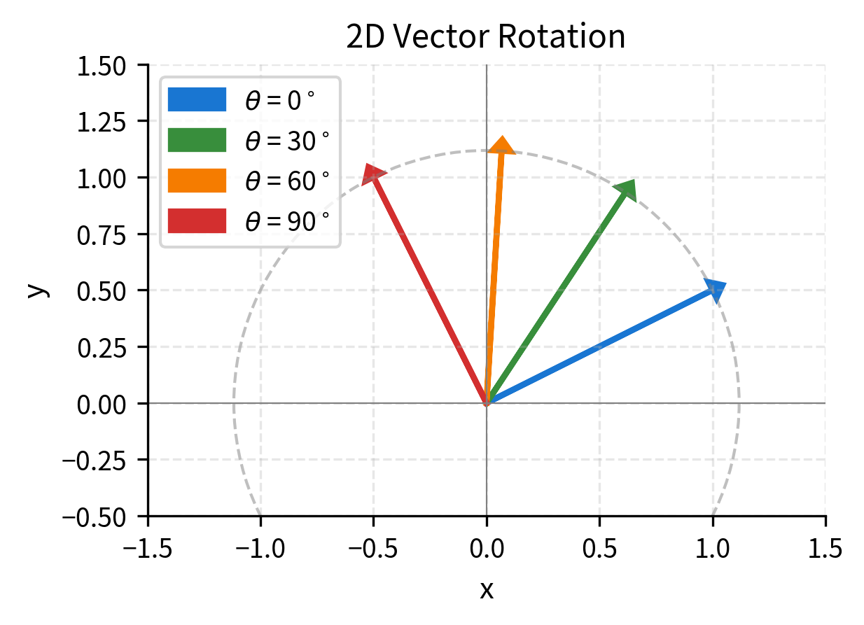
The dashed circle shows the path traced by the vector tip as it rotates. Crucially, the length (magnitude) never changes. Rotation is an isometry, a transformation that preserves distances.

Now let's see how rotation makes dot products depend on relative position. Take two 2D vectors $\mathbf{q}$ (query) and $\mathbf{k}$ (key). Rotate $\mathbf{q}$ by angle $m\theta$ (for position $m$) and $\mathbf{k}$ by angle $n\theta$ (for position $n$).

The dot product of the rotated vectors is:

where:

• $\mathbf{q}$: the query vector at position $m$
• $\mathbf{k}$: the key vector at position $n$
• $R(m\theta)$: rotation matrix that rotates by angle $m\theta$ (position times base angle)
• $R(n\theta)$: rotation matrix that rotates by angle $n\theta$

Using properties of rotation matrices, we can simplify this expression step by step:

The derivation proceeds as follows:

1. Rewrite the dot product as matrix multiplication: $R(m\theta)\mathbf{q} \cdot R(n\theta)\mathbf{k} = (R(m\theta)\mathbf{q})^T (R(n\theta)\mathbf{k}) = \mathbf{q}^T R(m\theta)^T R(n\theta) \mathbf{k}$
2. Apply the transpose-inverse property: The transpose of a rotation matrix equals its inverse, so $R(\theta)^T = R(-\theta)$. This gives us $R(m\theta)^T = R(-m\theta)$.
3. Apply the composition property: Multiplying two rotation matrices adds their angles, so $R(\alpha) R(\beta) = R(\alpha + \beta)$. Therefore $R(-m\theta) R(n\theta) = R((n-m)\theta)$.

The final result $\mathbf{q}^T R((n-m)\theta) \mathbf{k}$ depends only on the difference $(n-m)$, not on the absolute values of $m$ and $n$ separately.

This is remarkable. We encode absolute position through rotation angle, but the attention mechanism, which uses dot products, automatically extracts relative position. No architectural changes needed. No explicit bias terms. Just geometry.

Let's verify this numerically:

All four pairs have the same relative distance (2 positions apart), and their dot products are identical despite wildly different absolute positions. This confirms the relative position property holds numerically.

We've established that 2D rotation elegantly encodes relative position. But real transformer embeddings have hundreds or thousands of dimensions, not just 2. How do we extend this geometric insight to high-dimensional space?

The challenge is that rotations in high dimensions are more complex than in 2D. A naive approach might try to define a single rotation that affects all dimensions simultaneously, but this would be computationally expensive and wouldn't preserve the relative position property we just derived.

RoPE's solution is both clever and efficient: treat the $d$-dimensional embedding as $d/2$ independent pairs. A $d$-dimensional embedding is split into pairs: $(x_1, x_2)$, $(x_3, x_4)$, ..., $(x_{d-1}, x_d)$. Each pair is rotated independently as a 2D vector, and since the pairs don't interact, the relative position property holds for each pair separately. When we sum up the contributions from all pairs in a dot product, the overall score still depends only on relative position.

But here's where RoPE becomes truly expressive: each pair rotates at a different frequency. The first pair might rotate by $\theta$ per position, the second by $\theta/2$, the third by $\theta/4$, and so on. Think of it like the hour, minute, and second hands of a clock: each moves at a different rate, and together they can represent any time uniquely. Similarly, by using multiple frequencies, RoPE creates a rich encoding where different dimension pairs capture position information at different scales.

The rotation angle for dimension pair $i$ at position $m$ is:

where:

• $\theta_i(m)$: the rotation angle (in radians) for dimension pair $i$ at sequence position $m$
• $m$: the position in the sequence (0, 1, 2, ..., $n-1$ for a sequence of length $n$)
• $i$: the dimension pair index (0, 1, 2, ..., $d/2 - 1$)
• $d$: the total embedding dimension (must be even)
• $\theta_i = 1/10000^{2i/d}$: the base frequency for dimension pair $i$, which decreases exponentially as $i$ increases
• 10000: the base constant (same as in sinusoidal position encodings), chosen empirically for good performance

To understand why this formula creates a multi-scale representation, consider the exponent $2i/d$:

• When $i = 0$: $\theta_0 = 1/10000^0 = 1$ (fastest rotation, one radian per position)
• When $i = d/4$: $\theta_{d/4} = 1/10000^{0.5} = 1/100 = 0.01$ (slower rotation)
• When $i = d/2 - 1$: $\theta_{d/2-1} \approx 1/10000$ (slowest rotation)

This exponential decay means early dimension pairs (small $i$) rotate quickly, capturing fine-grained position differences, while later dimension pairs (large $i$) rotate slowly, capturing longer-range relationships.

The table shows the exponential decay: pair 0 completes a full cycle in about 6 positions (high frequency), while pair 3 takes over 600 positions (low frequency). This 100× difference in wavelength is what allows RoPE to encode positions at multiple scales simultaneously.

Let's visualize this frequency spectrum to see the exponential decay more clearly:

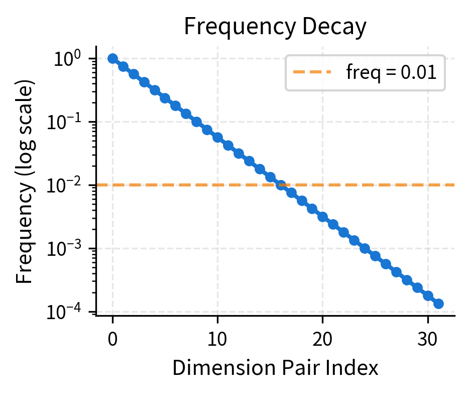
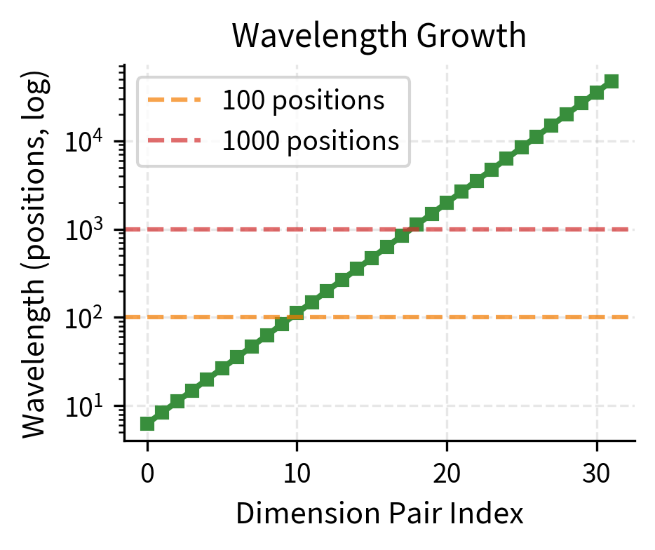
The wavelengths tell us how many positions before a dimension pair completes a full rotation (360°). Pair 0 completes a cycle in about 6 positions, while pair 3 takes over 600 positions. This exponential spread ensures RoPE can distinguish positions both locally and globally.

Now that we understand the individual components, let's bring everything together into the complete RoPE transformation. We've established three key ideas:

1. Rotation encodes position: Each position $m$ corresponds to a rotation angle $m\theta$
2. Dot products extract relative position: When query and key are rotated by different amounts, their dot product depends only on the angle difference
3. Multiple frequencies create richness: Different dimension pairs rotate at different rates, capturing both local and global position information

The complete RoPE formula combines these insights into a single elegant operation. Given a query or key vector $\mathbf{x} \in \mathbb{R}^d$ at position $m$, we apply RoPE as follows:

where:

• $\text{RoPE}(\mathbf{x}, m)$: the rotated vector, a function of both the input vector and position
• $\mathbf{x} \in \mathbb{R}^d$: the input query or key vector with $d$ dimensions
• $m$: the sequence position (integer index)
• $R(\theta_i \cdot m)$: the 2$\times$2 rotation matrix for angle $\theta_i \cdot m$, applied to dimension pair $i$
• $\theta_i = 1 / 10000^{2i/d}$: the base frequency for dimension pair $i$ (decreases exponentially with $i$)
• The block-diagonal structure means each 2$\times$2 rotation block operates independently on its corresponding dimension pair
• Empty off-diagonal blocks are zeros, so dimensions in different pairs don't interact during rotation

The large block-diagonal matrix applies different rotations to each dimension pair simultaneously. This is efficient because each 2D rotation is independent of the others, allowing for parallel computation.

Expanding the rotation for a single dimension pair $(x_{2i+1}, x_{2i+2})$:

where:

• $x_{2i+1}$, $x_{2i+2}$: the $(2i+1)$-th and $(2i+2)$-th components of the input vector (using 1-based indexing)
• $x'_{2i+1}$, $x'_{2i+2}$: the corresponding components after rotation
• $m\theta_i$: the rotation angle, which increases linearly with position $m$ at a rate determined by frequency $\theta_i$

Written out element-wise, the transformation is:

• $x'_{2i+1} = x_{2i+1} \cos(m\theta_i) - x_{2i+2} \sin(m\theta_i)$
• $x'_{2i+2} = x_{2i+1} \sin(m\theta_i) + x_{2i+2} \cos(m\theta_i)$

The matrix formulation we've developed is mathematically complete, but there's an even more elegant way to express RoPE using complex numbers. This isn't just a notational convenience: the complex perspective reveals the deep connection between rotations and exponentials, and leads to more efficient implementations.

The key insight is that a 2D rotation is equivalent to multiplication by a complex exponential. Every 2D vector $(x, y)$ can be viewed as a complex number $z = x + jy$, where $j$ is the imaginary unit. In this representation, rotating the vector by angle $\theta$ is simply multiplying by $e^{j\theta}$.

For the dimension pair $(x_{2i+1}, x_{2i+2})$, interpret them as the real and imaginary parts of a complex number:

where:

• $z_i$: a complex number representing dimension pair $i$
• $x_{2i+1}$: the real part (first element of the pair)
• $x_{2i+2}$: the imaginary part (second element of the pair)
• $j$: the imaginary unit (satisfying $j^2 = -1$)

Rotation by angle $\theta$ in the complex plane is achieved by multiplication:

where:

• $z'_i$: the rotated complex number
• $e^{j\theta}$: the complex exponential, a point on the unit circle at angle $\theta$
• $\cos\theta + j\sin\theta$: the expanded form via Euler's formula

For RoPE at position $m$, we apply this rotation with the position-dependent angle:

where:

• $m$: the sequence position
• $\theta_i$: the base frequency for dimension pair $i$
• $m \cdot \theta_i$: the total rotation angle (increases linearly with position)

This formulation is mathematically equivalent to the rotation matrix approach. The complex perspective leads to more concise code and can be more efficient on hardware with optimized complex number operations.

Let's verify that the complex formulation gives the same result as explicit rotation matrices:

The two implementations produce identical results (up to floating-point precision). The complex formulation is often preferred in practice because it's more concise and can leverage optimized complex number operations.

With both the matrix and complex formulations implemented, let's build intuition by visualizing how RoPE actually transforms embeddings. Understanding these patterns helps explain why RoPE is so effective at encoding position information.

We'll plot the rotation patterns for each dimension pair, tracking how a unit vector moves as position increases:

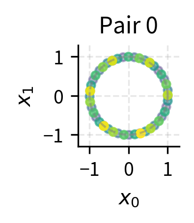
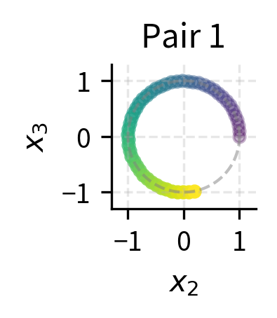
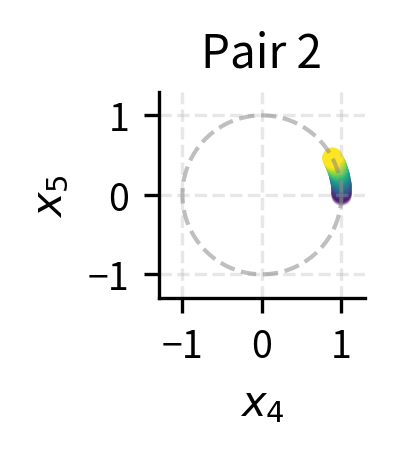
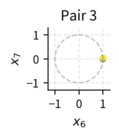
The color gradient (dark to light) shows increasing position. Pair 0 makes multiple full rotations within 50 positions, while Pair 3 barely completes an arc. This multi-frequency structure is what gives RoPE its expressiveness.

We've derived mathematically that RoPE should make attention scores depend only on relative position. Now let's verify this core property empirically and see what it looks like in practice.

The test is straightforward: create identical query and key vectors at different positions, apply RoPE, and compute attention scores. If RoPE works as intended, the scores should form a Toeplitz matrix, where each diagonal contains identical values. This structure proves that scores depend only on relative position (the difference between query and key positions), not on absolute positions.

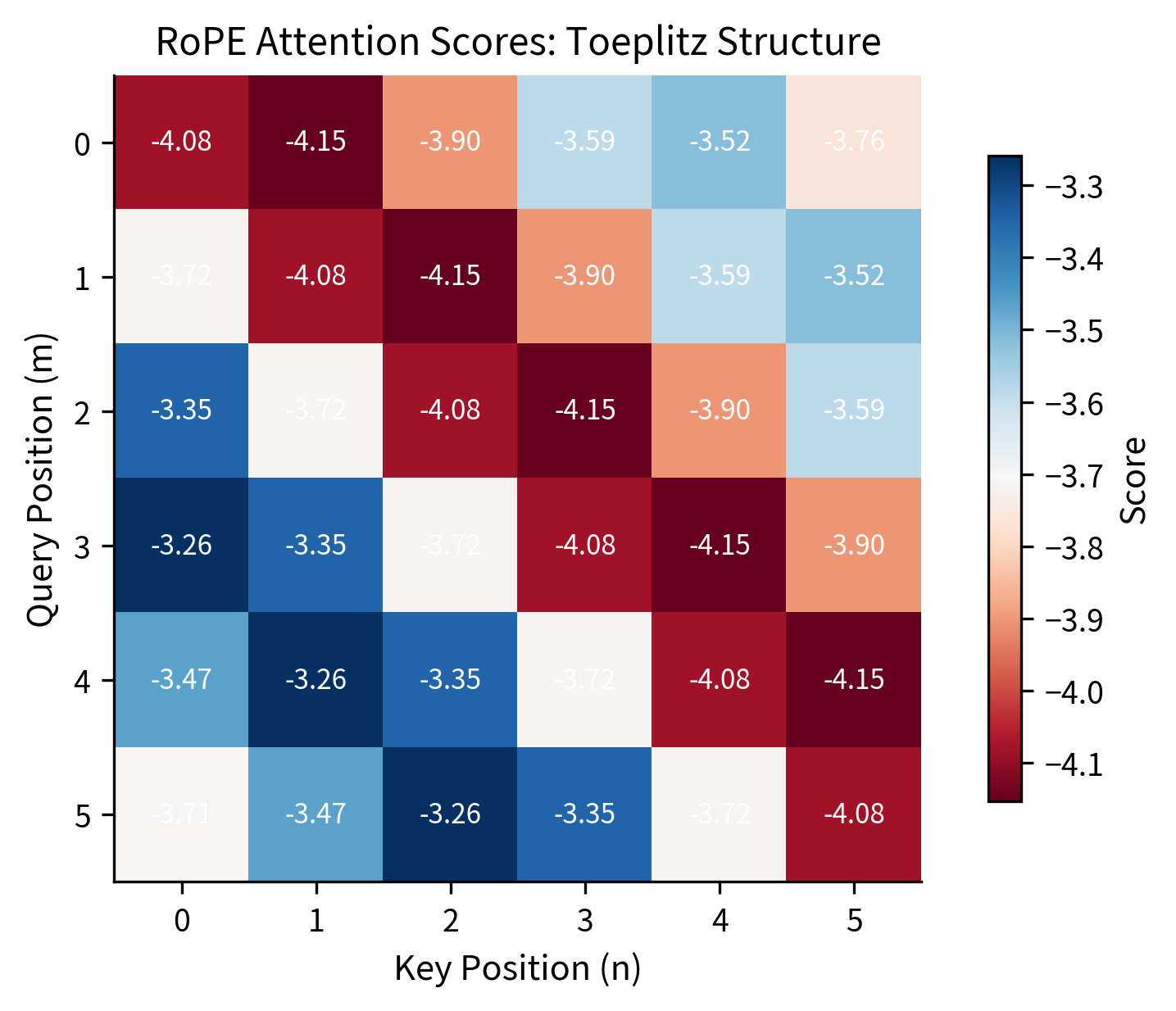
The Toeplitz structure is clear: all entries along each diagonal are identical. Position (0,0), (1,1), (2,2) all have the same score (relative distance 0). Position (0,1), (1,2), (2,3) all match (relative distance 1). This is the relative position property in action.

Let's verify numerically by extracting scores for each relative distance:

All standard deviations are effectively zero (within floating-point precision), confirming that scores at each relative distance are identical.

The Toeplitz structure tells us scores depend only on relative position, but how do they vary? Let's trace how the dot product changes as we increase the relative distance between query and key:

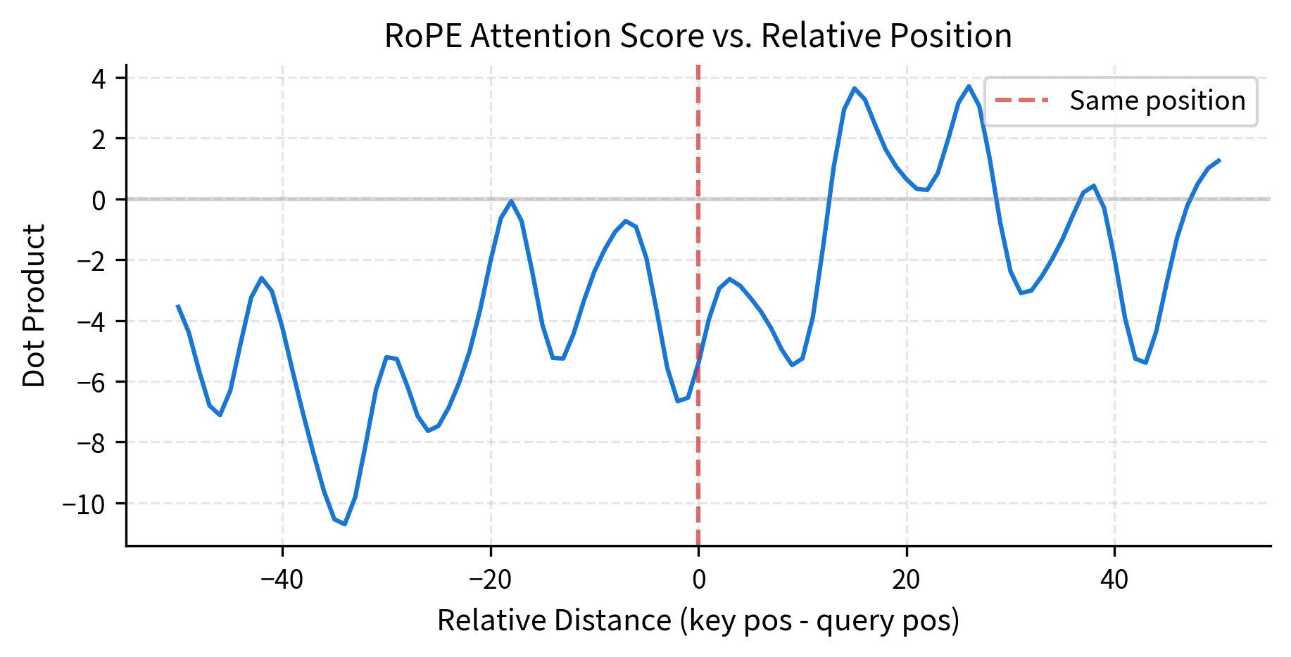
The oscillating pattern is characteristic of RoPE. The multiple frequencies create a complex interference pattern where some relative distances produce higher scores than others. This structure allows the model to learn position-dependent attention patterns during training.

The implementations we've shown so far process one token at a time, which is clear for understanding but inefficient in practice. Modern deep learning frameworks excel at vectorized operations, so we want to apply RoPE to all tokens in a sequence simultaneously.

The key insight is that we can precompute all rotation angles as a matrix and apply them through broadcasting. Instead of looping over positions and dimension pairs, we compute everything in parallel:

Let's verify this batch implementation matches the per-token version:

The maximum difference between implementations is on the order of $10^{-16}$, which is essentially machine epsilon for 64-bit floating point. This confirms that the batch implementation produces numerically identical results while being much more efficient through vectorization.

With efficient RoPE implementation in hand, let's see how it fits into a complete self-attention layer. The integration is remarkably clean: RoPE slots in between the QKV projections and the attention computation, requiring no architectural changes to the transformer.

Here's the complete flow:

1. Project input embeddings to Q, K, V using learned weight matrices
2. Apply RoPE to Q and K (but not to V)
3. Compute scaled dot-product attention as usual
4. Return the attention output

The critical detail is step 2: we rotate queries and keys but leave values untouched. Let's implement this:

Note that RoPE is applied only to queries and keys, not to values. This is because:

1. Queries and keys determine attention patterns: The dot product between them computes compatibility. RoPE makes this compatibility position-aware.
2. Values carry content: They should not be position-encoded because the content itself doesn't depend on position, only how much weight it receives.

The output confirms correct behavior: input of shape (8, 16) produces output of shape (8, 8) after projection to the query/key/value dimension. The attention weights form an 8×8 matrix where each row sums to exactly 1.0, confirming proper softmax normalization. The RoPE transformations are applied internally to queries and keys, making attention position-aware without changing the external interface.

The choice of frequencies is crucial to RoPE's effectiveness. Let's visualize how the multi-frequency structure creates unique position signatures:

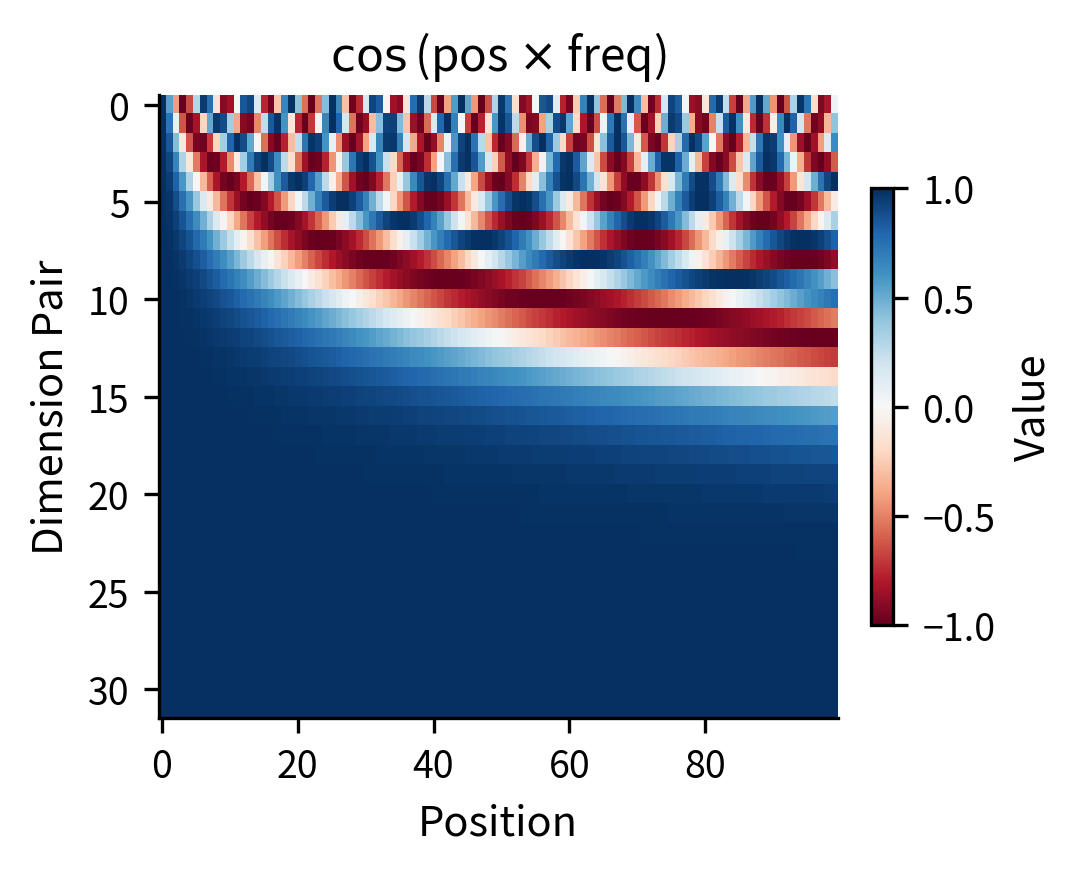
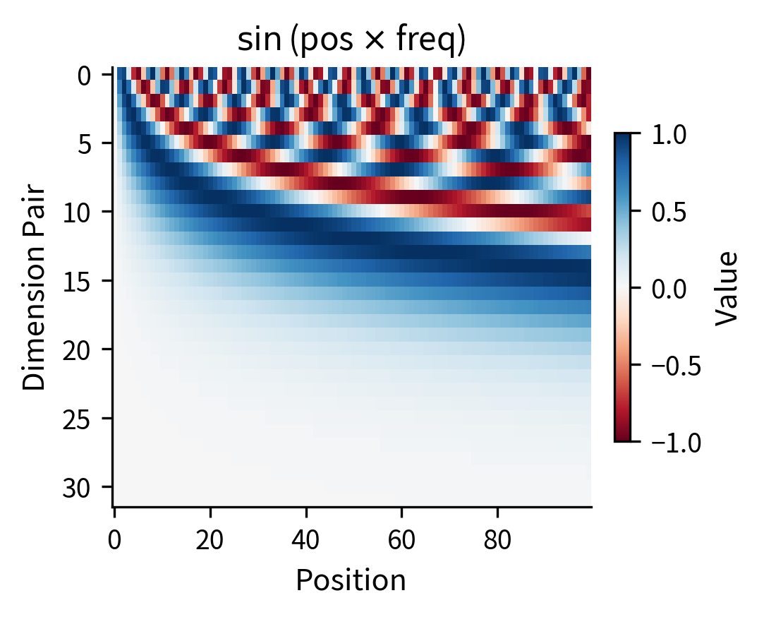
The heatmaps reveal the multi-scale nature of RoPE. Low-index dimension pairs (top rows) cycle rapidly, distinguishing nearby positions. High-index pairs (bottom rows) change slowly, providing a coarse position signal. This structure resembles sinusoidal position encodings since both use similar frequency patterns. The key difference is that sinusoidal encodings add position information to embeddings, while RoPE rotates the embeddings themselves.

Several properties make RoPE particularly effective:

Relative position by design. Unlike additive position encodings that must learn to extract relative position, RoPE provides it automatically through the geometry of rotations. The model doesn't need to learn that positions 5 and 7 are "2 apart"; the attention scores inherently reflect this.

Length generalization. Because RoPE encodes relative rather than absolute position, models can often generalize to longer sequences than seen during training. Position 1000 rotating relative to position 1002 works the same as position 0 rotating relative to position 2.

Computational efficiency. RoPE requires no additional parameters beyond the pre-computed frequencies. The rotation can be implemented as element-wise operations, making it very fast.

Compatibility with linear attention. Some efficient attention approximations rely on the inner product structure of attention. RoPE preserves this structure (rotation is a linear transformation), making it compatible with these methods.

Identical scores at identical relative distances, regardless of absolute position. This is why RoPE-based models can extrapolate to longer contexts more gracefully than models with absolute position encodings.

Let's visualize this length generalization property more comprehensively by testing many absolute position pairs:

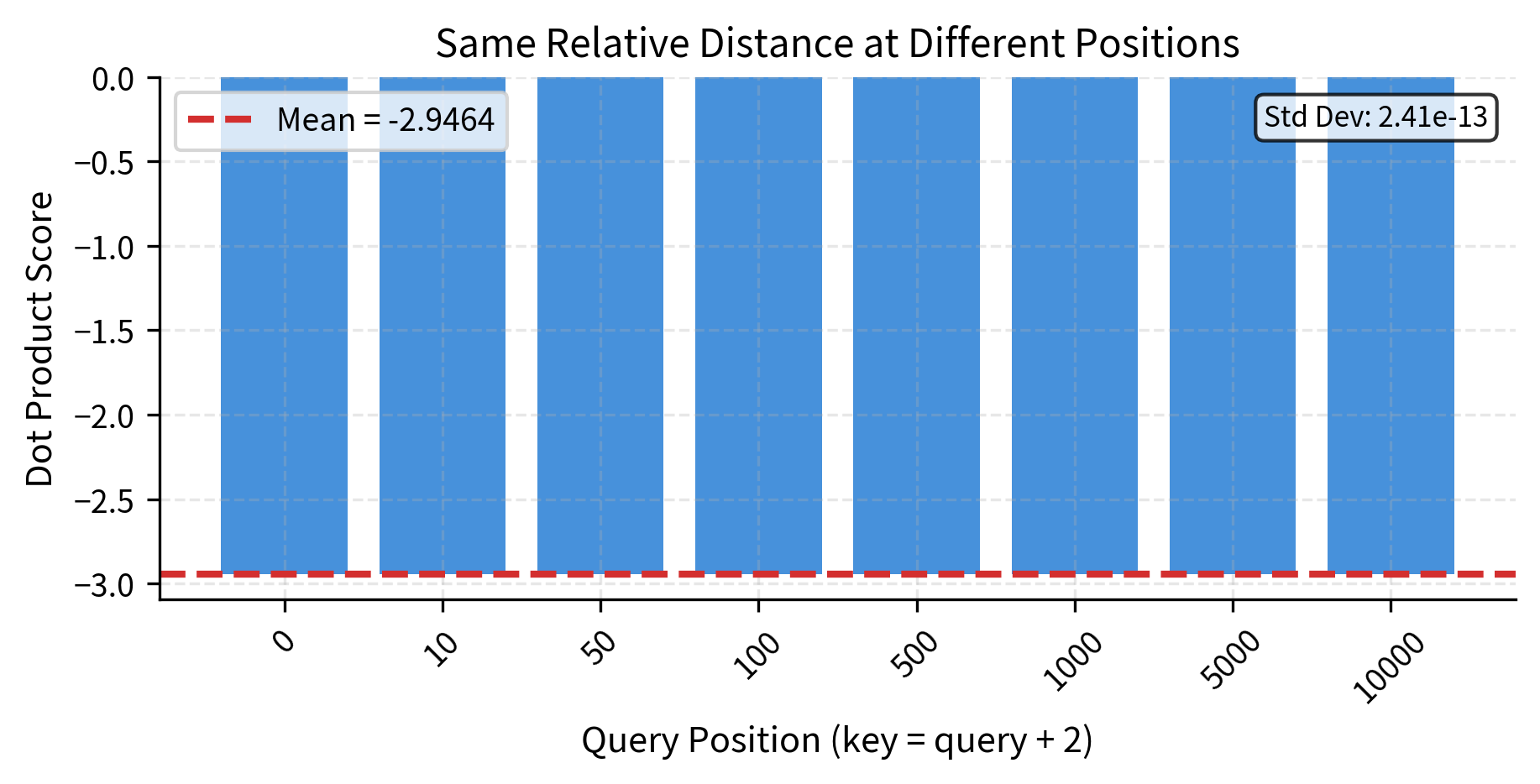
The nearly zero standard deviation confirms that RoPE perfectly preserves relative position information regardless of where in the sequence we look. This is the mathematical foundation for length generalization in RoPE-based models.

Let's position RoPE within the broader landscape of position encodings:

RoPE combines the parameter efficiency of sinusoidal encodings with the relative position benefits of learned relative encodings, without the architectural complexity. This balance explains its widespread adoption.

To make this comparison concrete, let's visualize how position similarity decays with distance for different encoding schemes:

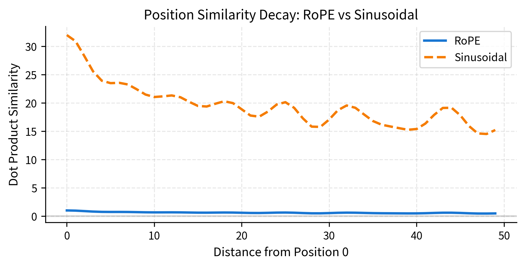
Both methods show oscillating similarity patterns due to their multi-frequency structure. The key difference: sinusoidal encodings add this pattern to the input, while RoPE modulates the attention computation directly through rotation.

Despite its elegance, RoPE has limitations worth understanding.

Frequency base sensitivity. The base (typically 10000) determines the frequency range. Models trained with one base may not transfer well to contexts requiring different frequency patterns. Recent work like YaRN and NTK-aware scaling addresses this by adjusting frequencies for longer contexts.

High-frequency aliasing. At very long positions, high-frequency dimension pairs may "wrap around" multiple times, potentially creating aliasing where distant positions appear similar. In practice, this is rarely problematic within reasonable context lengths, but it's a theoretical limitation.

Dimension divisibility. RoPE requires even-dimensional queries and keys since it operates on pairs. This is a minor constraint but must be considered in architecture design.

Training distribution effects. While RoPE theoretically supports any position, the model's other components (feed-forward networks, layer norms) are trained on a specific position distribution. Significant extrapolation may still degrade performance due to these other components, not RoPE itself.

These limitations are generally manageable. The community has developed extensions like Position Interpolation and NTK-aware RoPE that modify the frequency computation for better long-context performance. The core rotation mechanism remains unchanged.

When implementing RoPE in your models, these parameters control its behavior:

• d_model (embedding dimension): The total dimension of query and key vectors. Must be even since RoPE operates on dimension pairs. Common values range from 64 to 4096, typically matching the model's hidden dimension divided by the number of attention heads.

• base (frequency base): Controls the range of rotation frequencies. The default value of 10000 provides a good balance between local and global position sensitivity. Larger values (e.g., 100000) extend the effective context length by slowing all rotations; smaller values make the encoding more sensitive to nearby positions.

• theta_i (per-dimension frequency): Computed as $1/\text{base}^{2i/d}$ for dimension pair $i$. Not typically set directly, but understanding this helps diagnose behavior: the first pair rotates once per radian, while the last pair completes a full rotation over approximately $2\pi \times \text{base}$ positions.

• Position offset: Some implementations support a starting position offset for key-value caching during inference. This allows continuing generation from a specific position without recomputing RoPE for all previous positions.

Rotary Position Embedding encodes position through geometric rotation rather than additive signals. This approach elegantly captures relative position through the natural properties of dot products between rotated vectors.

Key takeaways:

• Rotation as position encoding. Each position corresponds to a rotation angle. Rotating query and key vectors embeds position information directly into their geometric relationship.

• Relative position emerges. When a rotated query at position $m$ attends to a rotated key at position $n$, the dot product depends only on $m - n$. Absolute positions cancel out through rotation mathematics.

• Multi-frequency structure. Different dimension pairs rotate at different frequencies, creating a rich position representation. High frequencies capture local position differences; low frequencies capture global structure.

• No additional parameters. Like sinusoidal encodings, RoPE uses deterministic frequencies based on dimension index. The only computation is the rotation itself.

• Applied to Q and K only. Values are not rotated because they carry content, not position information. Rotation affects attention patterns, not the content that flows through them.

• Good extrapolation. Because relative position is baked into the mechanism, models can often generalize to longer sequences than seen during training, though other model components may still limit this.

RoPE has become the dominant position encoding in modern large language models. Its combination of theoretical elegance, computational efficiency, and practical effectiveness makes it a foundational technique for transformer architectures. In the next chapter, we'll explore ALiBi, an alternative approach that adds relative position bias directly to attention scores.

Ready to test your understanding? Take this quick quiz to reinforce what you've learned about Rotary Position Embedding (RoPE).