

Explore how moving layer normalization before the sublayer (pre-norm) rather than after (post-norm) enables stable training of deep transformers like GPT and LLaMA.

This article is part of the free-to-read Language AI Handbook
Choose your expertise level to adjust how many terms are explained. Beginners see more tooltips, experts see fewer to maintain reading flow. Hover over underlined terms for instant definitions.
Pre-Norm vs Post-Norm
The original transformer paper placed layer normalization after the residual connection, a design choice known as post-norm. This seemed natural: apply the sublayer, add the residual, then normalize the combined result. But as researchers pushed transformers to greater depths, they discovered that this ordering creates training instabilities that become severe in very deep networks. The solution was elegantly simple: move the normalization before the sublayer. This pre-norm formulation has become the default in modern architectures like GPT and LLaMA, enabling stable training of models with hundreds of layers.
Understanding the difference between pre-norm and post-norm is essential for implementing transformers, diagnosing training issues, and choosing architectures. The choice affects not just stability but also the final model's behavior, with subtle trade-offs that practitioners should understand.
The Original Transformer: Post-Norm
The 2017 "Attention Is All You Need" paper introduced what we now call the post-norm configuration. In this design, each sublayer (attention or feed-forward) follows a specific pattern: apply the sublayer transformation, add the residual, then normalize.
In post-norm transformers, layer normalization is applied after the residual addition. For a sublayer function , the output is:
where:
- : the input representation (a -dimensional vector for each position)
- : the sublayer transformation (either self-attention or feed-forward network)
- : the residual connection, adding the original input to the sublayer output
- : layer normalization applied to the combined signal
- : the output of the block, which becomes the input to the next block
The intuition behind post-norm is straightforward. The sublayer computes its transformation, the residual connection preserves the original signal, and layer normalization ensures the combined output has stable statistics. Each component does one job, and they compose cleanly.
Let's implement a post-norm transformer block to see this in action:
The ordering is explicit: sublayer first, residual addition second, normalization third. This creates a clean signal flow where the normalized output is always what enters the next layer.
The output has approximately zero mean and unit variance (std 1), confirming that layer normalization has done its job. Regardless of what the sublayer computes or how the residual shifts the distribution, the final normalization step ensures stable statistics. This normalized output is what enters the next block in the network, preventing activation magnitudes from growing unboundedly.
The Pre-Norm Alternative
The pre-norm configuration emerged from research on training very deep networks. Instead of normalizing after the residual, pre-norm normalizes before applying the sublayer:
In pre-norm transformers, layer normalization is applied before the sublayer. For a sublayer function , the output is:
where:
- : the input representation (a -dimensional vector for each position)
- : layer normalization applied to the input before the sublayer
- : the sublayer transformation (either self-attention or feed-forward network), operating on the normalized input
- : the residual connection, adding the original (unnormalized) input to the sublayer output
- : the output of the block, which is not normalized
Notice the key difference: normalization happens inside the residual branch, not after the addition. This seemingly minor change has profound implications for gradient flow.
The ordering change is subtle but crucial: normalize, apply sublayer, add residual. The residual connection bypasses both the normalization and the sublayer, creating a direct gradient path from output to input.
Notice the key difference: the output statistics differ from the normalized values we saw with post-norm. The output is not normalized because the residual adds the original (unnormalized) input to the sublayer output. This accumulation behavior becomes important when we stack many blocks, as activations can grow in magnitude through the network.
Visualizing the Difference
The structural difference between pre-norm and post-norm becomes clearer when we visualize the computation graphs:
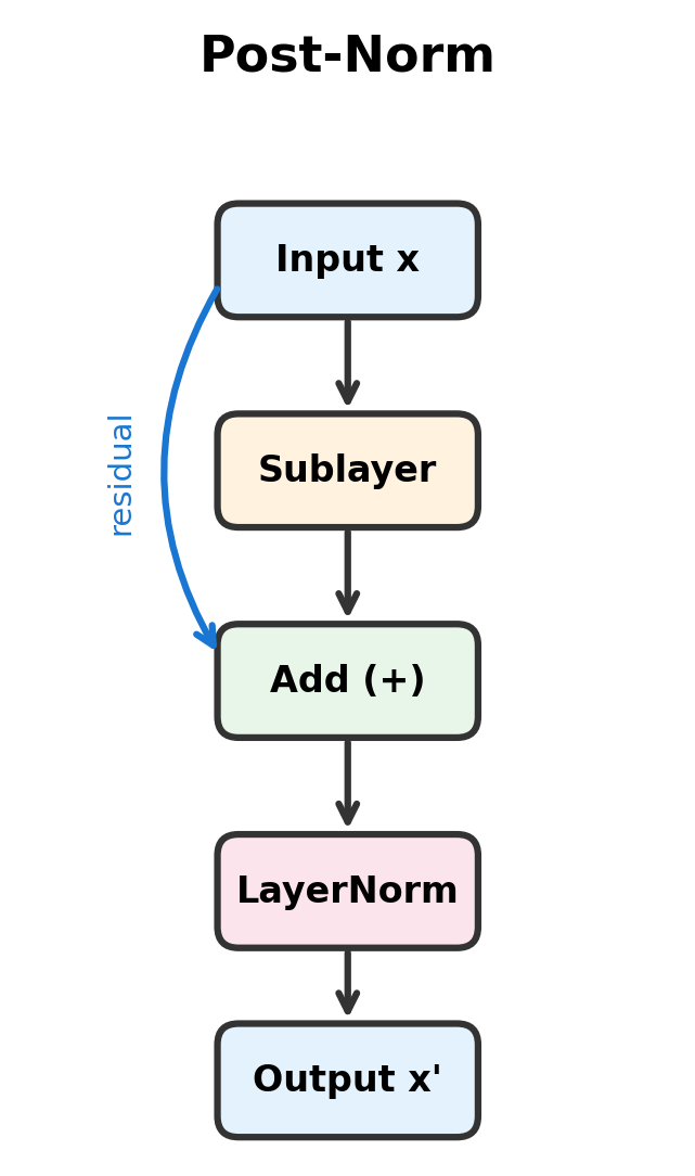
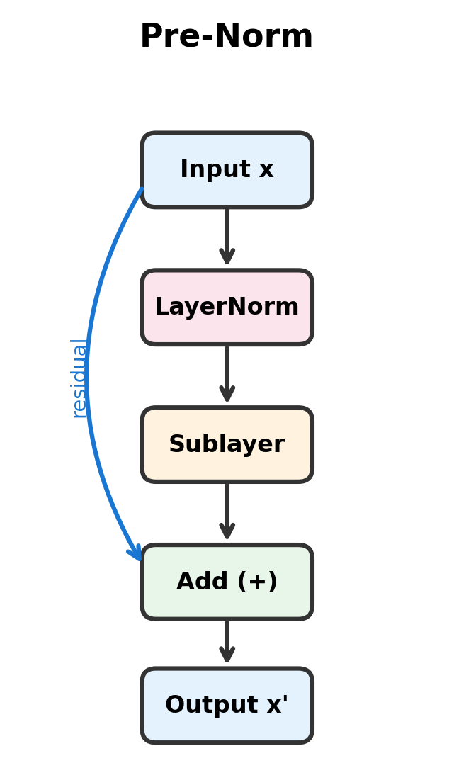
The diagrams reveal the fundamental difference. In post-norm, the residual enters the add block alongside the sublayer output, and layer normalization processes their sum. In pre-norm, the residual bypasses both layer normalization and the sublayer, creating a direct path from input to output.
Training Stability: The Gradient Flow Perspective
The practical motivation for pre-norm comes from training stability. While the forward pass differences we've seen are instructive, the real story unfolds during training, when gradients must flow backward through potentially hundreds of layers. Understanding this gradient flow explains why pre-norm enables stable training of very deep networks while post-norm struggles.
The Vanishing Gradient Problem in Deep Networks
Training neural networks requires computing how changes in each parameter affect the final loss. We do this through backpropagation: starting from the loss, we work backward through the network, computing gradients layer by layer using the chain rule.
Here's the challenge. The chain rule multiplies gradients together. If you have 100 layers and each layer slightly shrinks the gradient (say, by a factor of 0.99), the gradient reaching the first layer is of what it started as. If each layer shrinks it by 0.95, you get , and the earliest layers barely learn anything. This is the vanishing gradient problem.
The converse, exploding gradients, happens when each layer slightly amplifies the gradient. Even small amplification factors compound exponentially, leading to numerical overflow and unstable training.
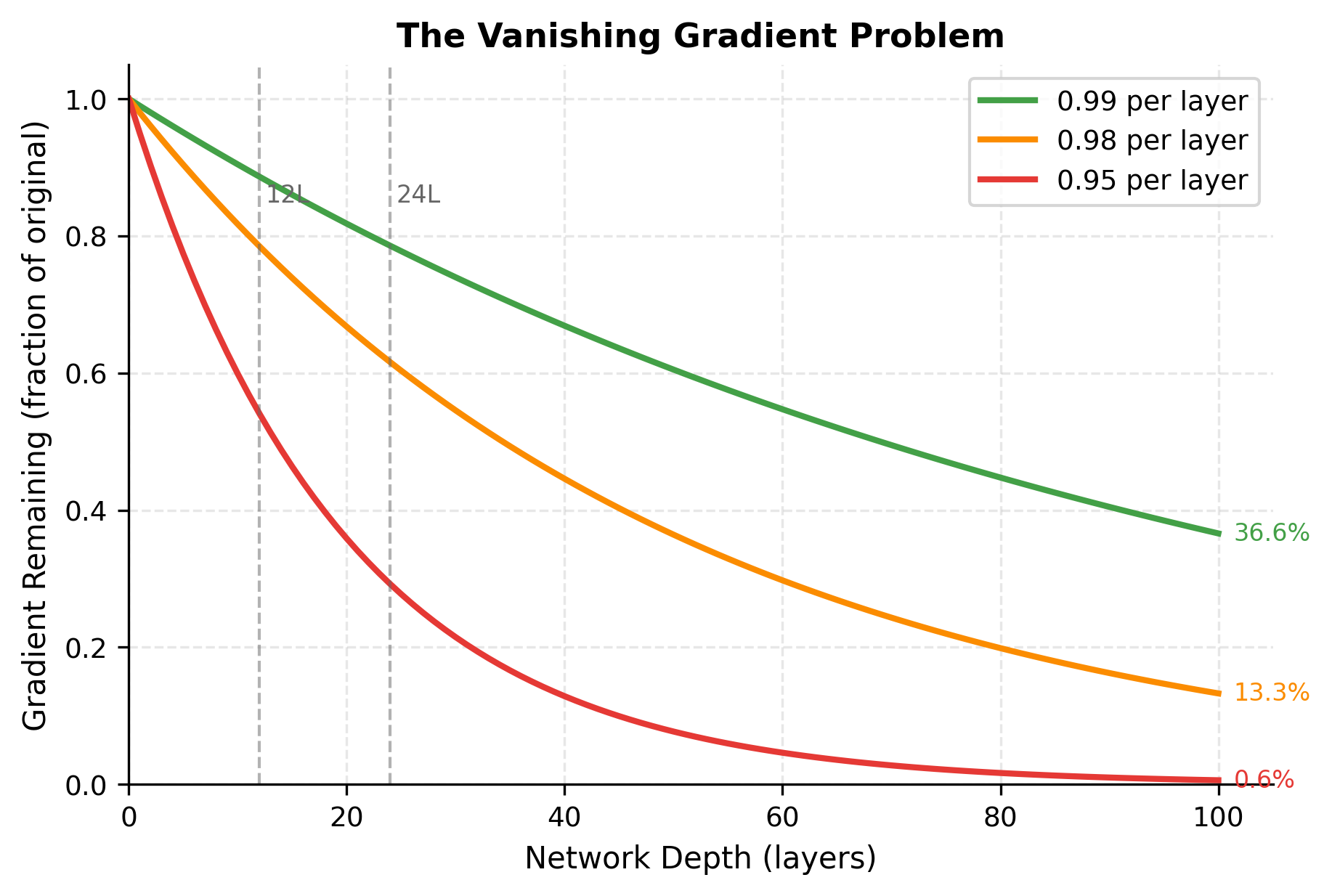
The visualization makes the exponential decay visceral. Even at the modest depth of 12 layers (BERT's configuration), a 2% per-layer reduction leaves only about 78% of the gradient. At 100 layers, a 5% reduction per layer is catastrophic, leaving less than 1% of the original gradient signal.
Residual connections were designed to address this problem by providing a direct path for gradients. But as we'll see, where you place the layer normalization determines whether this path remains truly direct.
Deriving the Gradient Flow
To understand the stability difference, we need to trace how gradients flow through each block type. Let's denote:
- : the loss function we're minimizing
- : the input to a transformer block
- : the output of the block
- : the gradient arriving from subsequent layers (we receive this during backpropagation)
- : the gradient we need to compute and pass to earlier layers
The chain rule tells us that . The key question is: what does look like for each block type?
Gradient Flow in Post-Norm
Recall the post-norm formulation: . To compute the gradient, we apply the chain rule from outside to inside:
- First, the gradient passes through LayerNorm
- Then, it splits into two paths: through the residual () and through the sublayer
Mathematically, this gives:
where:
- : the gradient of the loss with respect to the block input, which we want to compute
- : the gradient of the loss with respect to the block output (provided by the next layer during backpropagation)
- : the Jacobian of the layer normalization operation, a matrix that describes how small changes in the input to LayerNorm affect its output
- : the combined contribution from the residual path (the ) and the sublayer path
Notice the structure: the LayerNorm Jacobian appears as a multiplicative factor in the main gradient path. This is the crux of the instability problem. Even though LayerNorm has reasonably well-behaved gradients for a single layer (typically with eigenvalues close to 1), stacking many post-norm blocks means multiplying many of these Jacobians together. Small deviations from 1 compound across layers, leading to vanishing or exploding gradients in deep networks.
Gradient Flow in Pre-Norm
Now consider pre-norm: . The structural difference is subtle but crucial. Applying the chain rule:
- First, the gradient splits at the addition: one path goes through the residual (), another through the sublayer
- Only the sublayer path passes through LayerNorm
This yields:
where:
- : the gradient of the loss with respect to the block input
- : the gradient of the loss with respect to the block output
- : the gradient contribution from the direct residual path (since )
- : the Jacobian of the sublayer with respect to its (normalized) input
- : the Jacobian of layer normalization
The Gradient Highway
The key insight lies in that term inside the parentheses. In pre-norm, the gradient from the output has a direct, unmodified path back to the input. This path bypasses both the sublayer and the layer normalization entirely.
Think of it as a gradient highway: no matter what happens in the sublayer (vanishing activations, saturated nonlinearities, poorly conditioned weight matrices), the gradient can always flow back through the residual connection. The term ensures that at minimum, the full gradient reaches the input.
In post-norm, this highway doesn't exist in the same form. The LayerNorm Jacobian gates all gradient flow, including the residual path. If these Jacobians systematically shrink or grow gradients even slightly, the effects compound across many layers.
This mathematical property explains the empirical observations:
- Pre-norm networks train stably even at 100+ layers
- Post-norm networks require careful warmup schedules and smaller learning rates
- Pre-norm tolerates larger learning rates without diverging
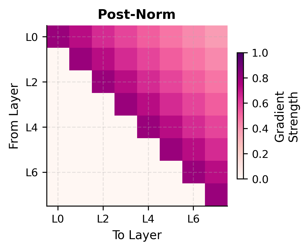
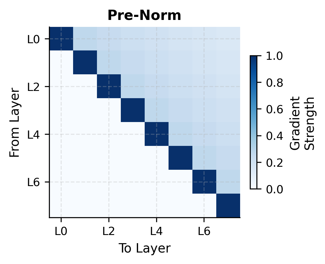
The heatmaps reveal the structural difference in gradient flow. In post-norm, gradient strength decays as it travels backward through layers, with no escape from the cascading LayerNorm Jacobians. In pre-norm, the bright diagonal represents the gradient highway: full-strength gradients flowing directly from any layer's output to its input, bypassing all intermediate transformations.
Let's simulate this difference with a numerical experiment:
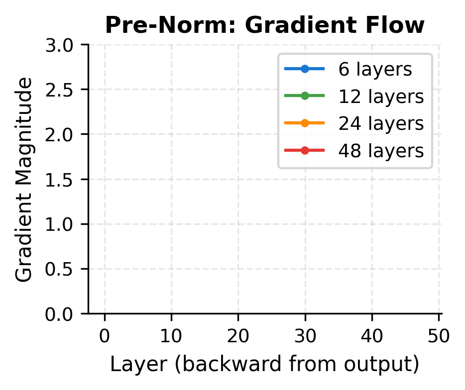
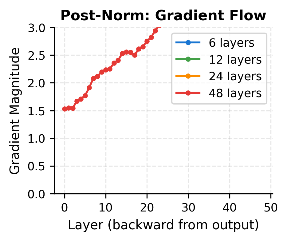
The visualization illustrates the stability difference. Pre-norm maintains consistent gradient magnitudes across all depths because the residual connection provides a direct gradient path. Post-norm gradients tend to decay in deeper networks, making optimization more challenging.
Output Scale: An Important Trade-off
Pre-norm's stability advantage comes with a trade-off: the output of each block accumulates without normalization. This can lead to growing activation magnitudes as we stack more layers.
Let's measure this effect:
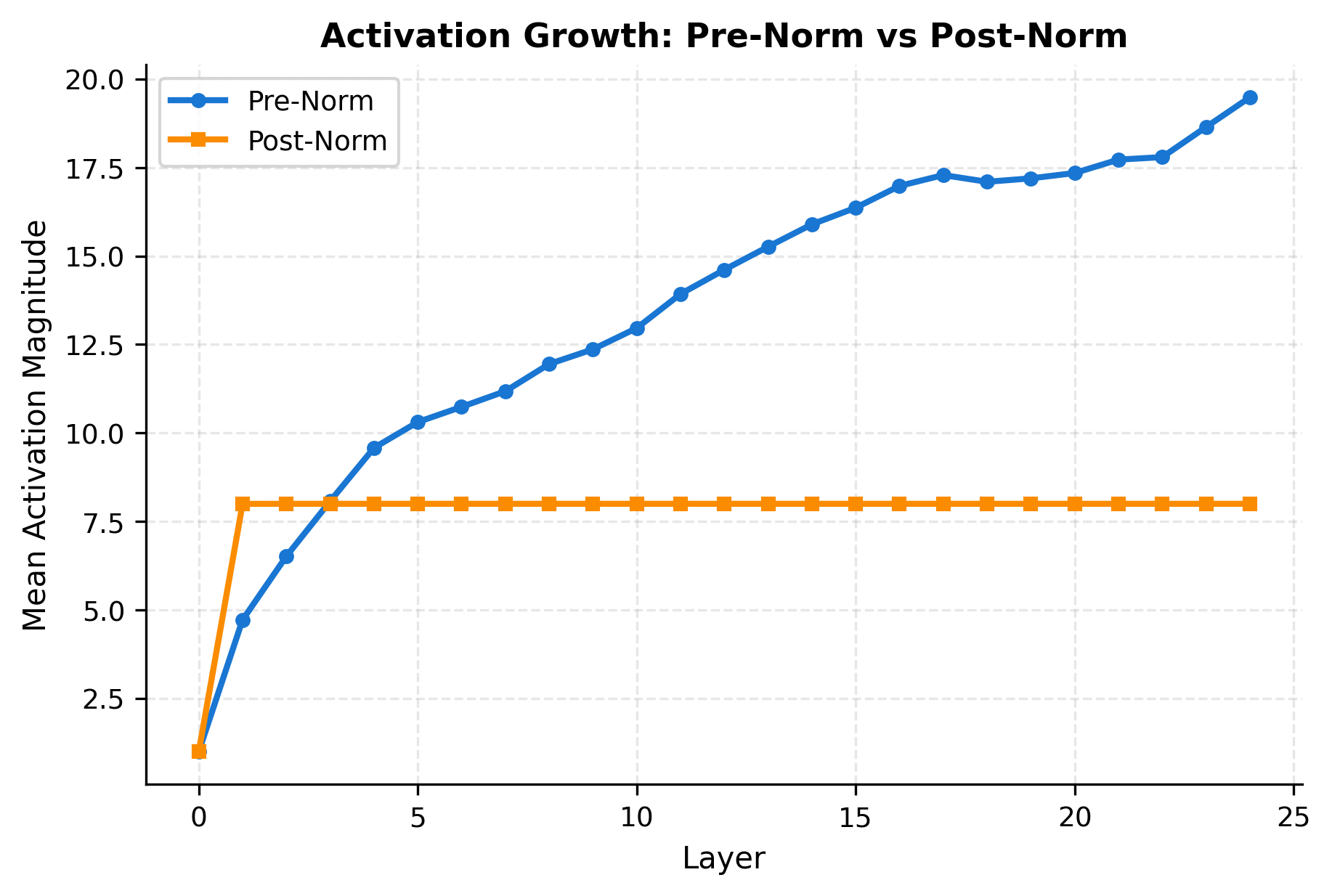
The growth in pre-norm isn't necessarily problematic, as the final layer normalization (applied before the output projection in most architectures) handles the accumulated magnitude. However, it does mean that numerical precision matters more in very deep pre-norm networks.
To understand where this growth comes from, we can decompose the output into contributions from the original input and each sublayer:
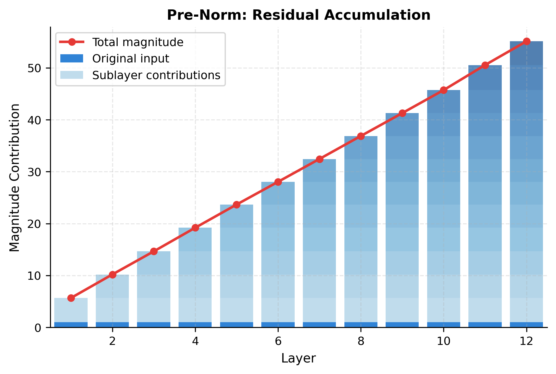
The decomposition reveals the structure of pre-norm's activation growth. The original input signal (dark blue) persists unchanged through all layers, which is the residual connection at work. Each sublayer adds its own contribution on top, and these contributions accumulate. The total magnitude (red line) grows steadily, but this growth is predictable and well-behaved, making it easy to compensate for with a final normalization.
Modern Architectures: The Pre-Norm Consensus
The empirical evidence strongly favors pre-norm for training stability, especially in large models. Let's examine how major architectures make this choice:
| Architecture | Norm Placement | Notes |
|---|---|---|
| Original Transformer | Post-Norm | First formulation, requires warmup |
| GPT-2, GPT-3 | Pre-Norm | Enabled stable training of large models |
| BERT | Post-Norm | Relatively shallow (12/24 layers) |
| RoBERTa | Post-Norm | Follows BERT architecture |
| T5 | Pre-Norm | Stable training for encoder-decoder |
| LLaMA, LLaMA 2 | Pre-Norm | Uses RMSNorm variant |
| PaLM | Pre-Norm | Parallel attention variant |
| GPT-4 (likely) | Pre-Norm | Standard for modern LLMs |
The pattern is clear: newer and larger models overwhelmingly choose pre-norm. The stability benefits outweigh any theoretical concerns about activation accumulation.
The Final Layer Norm
Pre-norm architectures typically add a final layer normalization after all transformer blocks but before the output projection. This serves two purposes: it normalizes the accumulated activations, and it provides a consistent interface for the output layer.
Despite passing through 12 transformer blocks (each adding residual contributions), the final output magnitude remains controlled. The final layer normalization ensures that regardless of how activations accumulated through the network, the output has well-controlled statistics suitable for the output projection. This design pattern is why pre-norm architectures include a final LayerNorm before the language modeling head.
Initialization Considerations
The choice between pre-norm and post-norm affects how we should initialize the network. Post-norm requires more careful initialization because gradients must flow through the normalization layers.
For pre-norm, a common approach is to scale the output projection of each sublayer by a factor related to the network depth:
The residual scale factor of approximately 0.14 significantly reduces the contribution of each sublayer's output. With 24 layers (and 2 sublayers per block, hence 48 residual additions), this scaling prevents the accumulated sum from exploding. The GPT-2 paper introduced this technique specifically to enable training of deeper pre-norm networks.
Learning Rate Sensitivity
Post-norm architectures are notoriously sensitive to learning rate choices. Large learning rates can cause training to diverge, necessitating careful warmup schedules.
Pre-norm is more forgiving because the direct gradient path through residual connections prevents gradient explosion. This allows training with larger learning rates and simpler schedules.
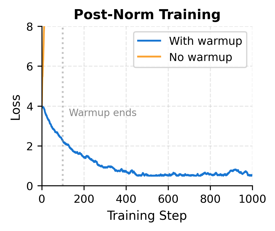
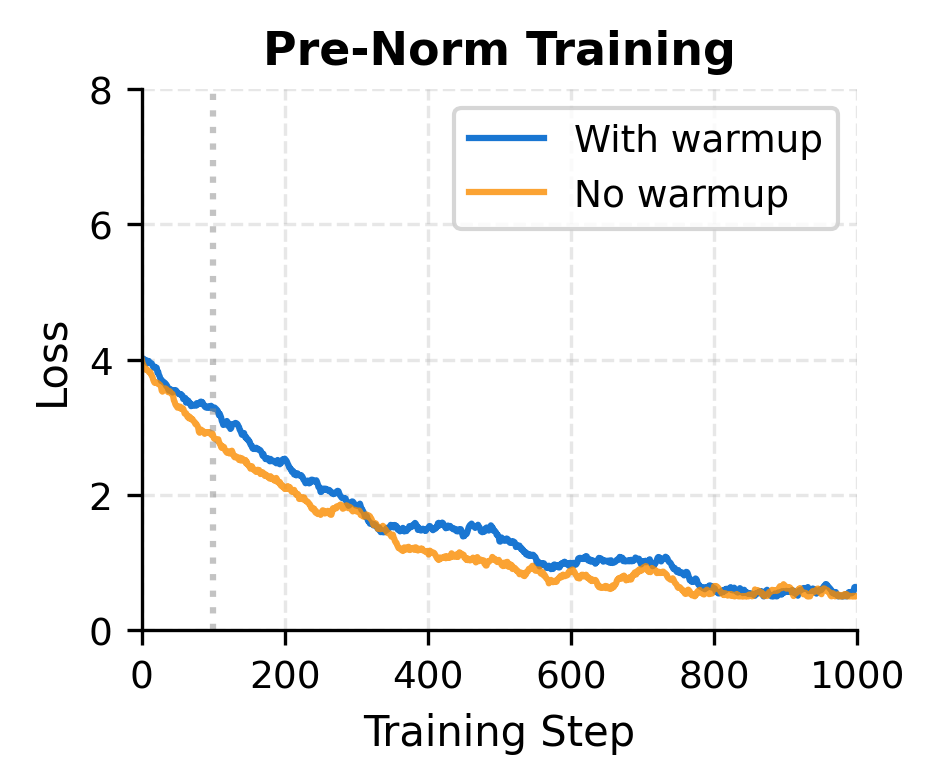
The simulated training curves illustrate the practical difference. Post-norm without warmup experiences immediate instability: the gradient explosion causes the loss to spike and training to fail. With warmup, the gradual learning rate increase gives the optimizer time to find a stable path. Pre-norm, by contrast, handles both scenarios gracefully because the gradient highway prevents the cascading instabilities that plague post-norm.
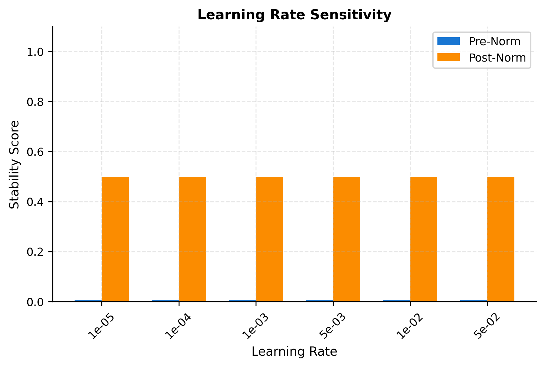
The stability comparison shows that pre-norm tolerates higher learning rates. This translates to faster convergence in practice, as larger learning rates allow taking bigger optimization steps.
When to Use Each Variant
Despite the modern consensus favoring pre-norm, there are situations where post-norm might be appropriate:
Use Pre-Norm when:
- Training deep networks (more than 12 layers)
- Building large language models (GPT-style)
- You want simpler hyperparameter tuning
- Training without extensive warmup periods
- Prioritizing training stability
Consider Post-Norm when:
- Working with shallow networks (12 layers or fewer)
- Fine-tuning existing post-norm models (like BERT)
- Reproducing results from older papers
- Situations where final representation normalization is critical
The theoretical argument for post-norm is that normalized outputs at each layer provide a cleaner signal for subsequent processing. Some researchers have found that post-norm achieves slightly better final performance when training succeeds, though the stability challenges often make this advantage inaccessible in practice.
Hybrid Approaches
Recent work has explored combining the benefits of both approaches. One variant uses post-norm with scaled residuals:
Another approach, used in some recent models, applies normalization both before and after the sublayer:
These hybrid approaches add complexity but can provide benefits in specific situations, particularly for extremely deep or wide networks.
Implementation Comparison
Let's implement both variants in a clean, comparable format that highlights their differences:
Even after just one block, the difference is visible. The post-norm output magnitude is close to (the expected magnitude for a normalized -dimensional vector), while pre-norm's output reflects the accumulation of the input and sublayer contributions. This difference compounds across many layers, which is why the architectural choice matters significantly for deep networks.
Limitations and Impact
The pre-norm versus post-norm choice exemplifies a common pattern in deep learning architecture design: seemingly minor structural changes can have profound effects on trainability. Pre-norm solved the training stability challenges that limited early transformer scaling, directly enabling the large language models that define modern NLP.
The main limitation of pre-norm is the accumulating activation scale through the network. While the final layer normalization handles this for most purposes, it can create numerical precision challenges in extremely deep networks (hundreds of layers). Some architectures address this with periodic intermediate normalization or careful scaling of residual contributions.
Post-norm's limitation is its training instability for deep networks. The requirement for warmup schedules and careful hyperparameter tuning increases the complexity of training pipelines. For practitioners working with pre-trained models like BERT, the post-norm design is fixed, and fine-tuning inherits these stability considerations.
The broader impact of understanding normalization placement extends beyond transformers. Similar considerations apply to any deep residual network: where you normalize relative to the residual connection fundamentally changes how gradients flow. This principle guides architecture design across computer vision, speech processing, and other domains.
Key Parameters
When implementing pre-norm or post-norm transformer blocks, these parameters control the behavior and stability:
-
norm_type: Choice between"pre"or"post". Pre-norm places LayerNorm before the sublayer; post-norm places it after the residual addition. Modern large models (GPT, LLaMA) use pre-norm for stability. -
eps(LayerNorm epsilon): Small constant (typically1e-5or1e-6) added to the variance for numerical stability. Prevents division by zero when variance is very small. -
gamma,beta(LayerNorm parameters): Learnable scale and shift parameters. Initialized to ones and zeros respectively, allowing the model to learn the optimal normalization behavior for each layer. -
residual_scale: For pre-norm networks, scaling the output of sublayers by a factor like (where is the number of layers) prevents activation explosion. GPT-2 uses this technique. -
n_layers: Network depth directly impacts the choice between pre-norm and post-norm. Networks deeper than 12 layers benefit significantly from pre-norm's gradient stability. -
learning_rate: Post-norm requires smaller learning rates and warmup schedules. Pre-norm tolerates larger learning rates (often 3-10x higher) and simpler schedules.
Summary
The placement of layer normalization relative to residual connections determines whether a transformer uses pre-norm or post-norm architecture. This choice significantly impacts training dynamics, stability, and practical usability.
Key takeaways from this chapter:
-
Post-norm normalizes after the residual addition: The original transformer design applies normalization to the sum of the sublayer output and residual. This ensures each layer produces normalized outputs but can create gradient flow challenges in deep networks.
-
Pre-norm normalizes before the sublayer: Moving normalization inside the residual branch provides a direct gradient path through the residual connection. This enables stable training of very deep networks without complex warmup schedules.
-
Gradient highways explain stability: The term from the residual connection in pre-norm ensures gradients can flow backward without attenuation, regardless of sublayer behavior. This mathematical property is why pre-norm trains more stably.
-
Activation accumulation is the trade-off: Pre-norm outputs are not normalized, leading to growing activation magnitudes. A final layer normalization before the output projection addresses this for most purposes.
-
Modern architectures favor pre-norm: GPT, LLaMA, and most large language models use pre-norm due to its stability benefits. Post-norm persists in some encoder models like BERT where network depth is more modest.
-
Learning rate tolerance differs: Pre-norm allows training with larger learning rates and simpler schedules. Post-norm requires careful warmup and learning rate selection to avoid divergence.
In the next chapter, we'll explore feed-forward networks, the other major component of transformer blocks alongside attention. Understanding how these two components work together completes the picture of transformer block architecture.
Quiz
Ready to test your understanding? Take this quick quiz to reinforce what you've learned about pre-norm and post-norm transformer architectures.

Comments