

Learn how GLUs transform feed-forward networks through multiplicative gating. Understand SwiGLU, GeGLU, and the parameter trade-offs that power LLaMA, Mistral, and other state-of-the-art language models.

This article is part of the free-to-read Language AI Handbook
Choose your expertise level to adjust how many terms are explained. Beginners see more tooltips, experts see fewer to maintain reading flow. Hover over underlined terms for instant definitions.
Gated Linear Units
The standard feed-forward network in transformers applies a simple formula: expand the dimension, apply an activation function, contract back. This works, but researchers discovered something better. By adding a gating mechanism, where one pathway controls how much of another pathway passes through, the FFN becomes significantly more expressive. This insight, borrowed from recurrent neural networks, has become the default choice in modern large language models.
Gated Linear Units (GLUs) replace the single nonlinearity in the FFN with a product of two linear projections, one of which passes through an activation function to produce "gate" values between 0 and 1. These gates control information flow: they can fully pass, partially attenuate, or completely block the signal from the other pathway. This multiplicative interaction creates richer representations than a simple pointwise nonlinearity.
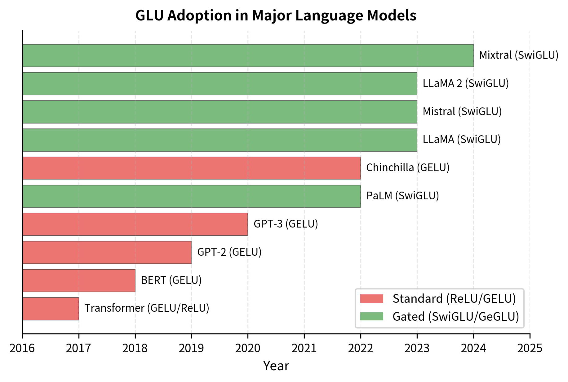
The impact has been dramatic. LLaMA, PaLM, Mistral, and virtually every state-of-the-art LLM now uses a GLU variant. The SwiGLU formulation has become particularly dominant, offering improved training dynamics and better downstream performance at comparable parameter counts. This chapter explains why gating works, how to implement it, and the trade-offs that come with this more sophisticated architecture.
The Gating Mechanism
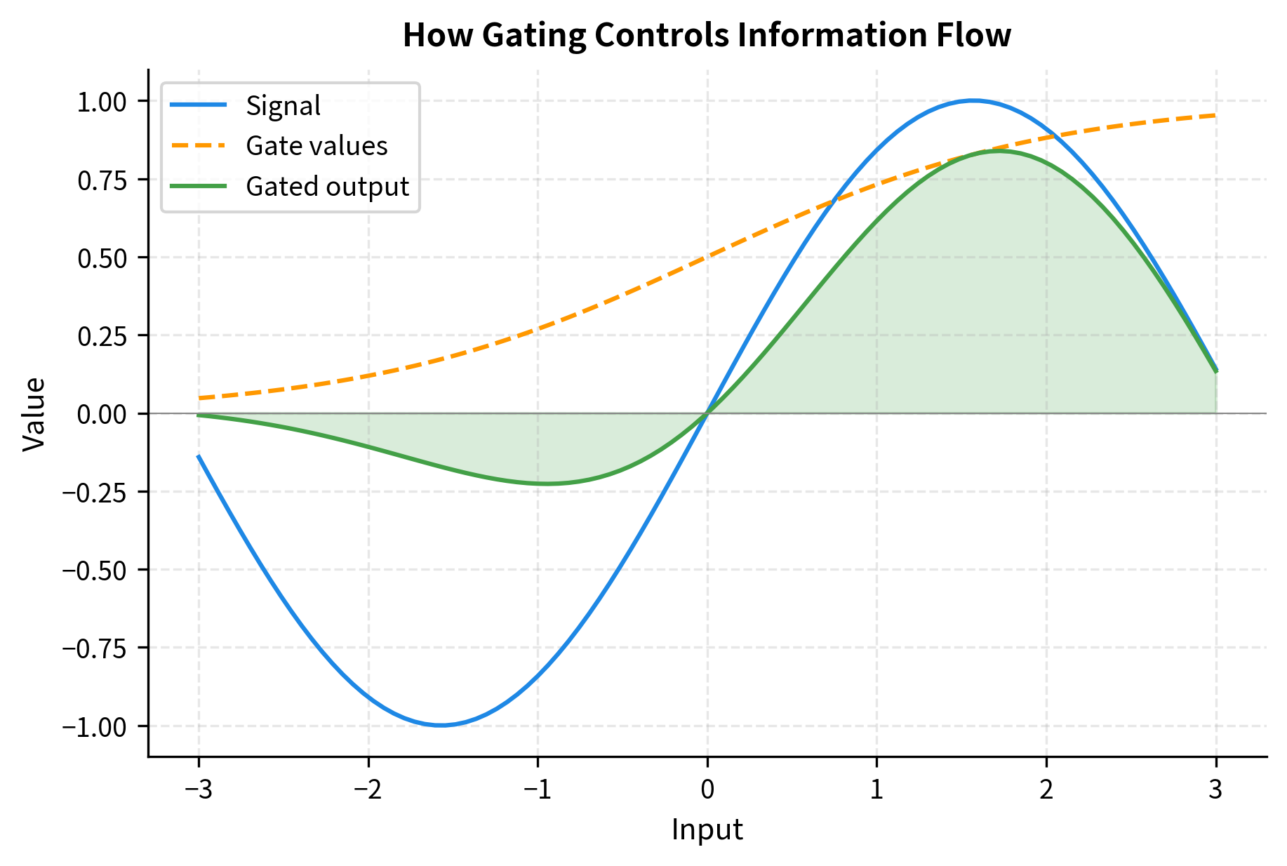
Before diving into the GLU formulation, let's understand what gating means. A gate is a learned mechanism that controls information flow. The idea comes from LSTM networks, where gates solve the vanishing gradient problem by allowing gradients to flow unimpeded through time. In the context of feed-forward layers, gates serve a different purpose: they create multiplicative interactions that increase expressiveness.
A gate is a learned function that produces values in a bounded range (typically 0 to 1) that multiply another signal. When the gate outputs 0, the signal is blocked; when it outputs 1, the signal passes through unchanged. Values between 0 and 1 attenuate the signal proportionally.
Consider the difference between additive and multiplicative interactions. A standard FFN uses purely additive interactions: the output is a weighted sum of transformed features. Multiplication introduces second-order terms. When you multiply two linear functions of the input, you get terms like , which allows the network to model interactions between features that addition alone cannot capture.
The power of gating becomes clear when you consider what a gate can learn. A gate can learn to be "always open" (outputting 1), in which case the GLU behaves like a standard linear layer. It can learn to be "always closed" (outputting 0), effectively pruning that dimension. Or it can learn input-dependent behavior, opening for some patterns and closing for others. This flexibility subsumes the standard FFN as a special case while enabling much richer transformations.
The GLU Formulation
Now that we understand what gating does, let's formalize how it works mathematically. The Gated Linear Unit was introduced by Dauphin et al. in 2017 for language modeling, and its elegance lies in a simple but powerful insight: instead of applying an activation function to transform features, let the network learn which features to keep and which to suppress.
The Core Idea: Two Pathways, One Output
Standard neural network layers compute a single transformation of their input and apply an activation function. GLU takes a fundamentally different approach: it computes two separate linear projections of the same input and combines them through multiplication. One projection produces the "values" we want to transmit, while the other produces "gates" that control how much of each value passes through.
Think of it like a mixing console in a recording studio. Each channel has both a signal (the audio content) and a fader (the volume control). The final output for each channel is the signal multiplied by the fader position. The GLU works the same way, but learns both the signals and the fader positions from data.
The Mathematical Formulation
The original GLU formula captures this two-pathway structure:
Let's unpack each component to understand what it contributes:
The Value Pathway:
The first term computes a linear transformation of the input. This is the "content" that we might want to pass through to the next layer. Without the gate, this would just be a standard linear layer:
- : the input vector (a token's representation)
- : the "value" projection weights that transform the input
- : the value projection bias
The Gate Pathway:
The second term computes another linear transformation of the same input, but passes it through the sigmoid function to produce gate values:
- : the "gate" projection weights (separate from )
- : the gate projection bias
- : the sigmoid activation function, which squashes values to the range
- : the output dimension of each projection
The Combination: (Element-wise Multiplication)
The symbol denotes the Hadamard product, which simply multiplies corresponding elements. If the value pathway produces and the gate pathway produces , the output is .
Why Sigmoid for Gating?
The sigmoid function produces values between 0 and 1, making it a natural choice for gating:
where is the input value (applied element-wise when the input is a vector). The sigmoid's behavior at extreme values is what makes it effective as a gate:
- As , (gate closes completely)
- As , (gate opens fully)
- At , (gate is half-open)
When is close to 0, the corresponding element of is blocked, meaning that dimension contributes nothing to the output. When it's close to 1, the element passes through unchanged. Values between 0 and 1 allow partial transmission, giving the network fine-grained control over information flow.

From Theory to Code
Let's implement the basic GLU and see these components in action:
The output range shows that GLU produces both positive and negative values, unlike ReLU which only produces non-negative outputs. This is because the sigmoid gate modulates but doesn't constrain the sign of the value pathway.
The Dimension Trade-off
Notice something important about GLU's output dimension. If we project from to , we get outputs, not . This is because we use two projections (value and gate), each producing dimensions, and multiply them together element-wise to get outputs. The multiplication combines the two pathways rather than concatenating them.
This has significant implications for parameter efficiency that we'll explore shortly. First, let's see how GLU fits into the larger transformer architecture.
GLU in the Feed-Forward Network
With the GLU mechanism understood, our next step is integrating it into the transformer's feed-forward network. This requires adapting the standard two-layer FFN architecture, and understanding this integration reveals why GLU is such a natural fit for transformers.
Recalling the Standard FFN
The standard FFN applies a simple pattern: expand the dimension, apply nonlinearity, contract back:
where is the input, and are weight matrices, and are bias vectors, and is a nonlinear activation function (e.g., ReLU or GELU).
The key insight is that the nonlinearity is applied after the expansion. This creates a high-dimensional feature space where the nonlinearity can carve out complex decision boundaries, before projecting back to the original dimension.
Replacing Activation with Gating
GLU replaces the simple activation function with something more sophisticated: a learned gating mechanism. Instead of uniformly transforming all features with the same nonlinearity, GLU lets the network selectively amplify or suppress features based on the input itself:
Let's trace through what each component does in this context:
- Expansion to Hidden Space: Both and project the input from to the larger hidden dimension
- Gated Combination: The sigmoid-gated multiplication produces a -dimensional hidden representation
- Contraction Back: projects back to for the residual connection
The variables are:
- : input from attention/normalization
- : the two projection matrices for value and gate
- : corresponding bias vectors
- : output projection back to model dimension
- : output bias
The Parameter Cost
Notice that the GLU FFN requires three weight matrices (, , and ) instead of the standard FFN's two ( and ). This means GLU-based FFNs have 50% more parameters for the same hidden dimension. We'll analyze this trade-off in detail later and see how modern models address it.
The output shape matches the input shape, confirming that the GLU FFN correctly projects back to the model dimension. This dimensional consistency is essential for the residual connection that adds the FFN output back to its input in a transformer block.
SwiGLU: The Modern Standard
The original GLU with sigmoid gating works, but researchers discovered an even better formulation. SwiGLU, introduced by Shazeer in 2020, has become the dominant choice in modern LLMs, powering LLaMA, Mistral, and virtually every frontier model. Understanding why SwiGLU outperforms the original GLU reveals important insights about activation function design.
The Limitation of Sigmoid Gating
Recall that the original GLU uses sigmoid to produce gate values between 0 and 1. While this works well for controlling information flow, sigmoid has a subtle limitation: it saturates at both ends. For very large positive inputs, the gate is always ~1; for very large negative inputs, always ~0. This saturation can limit expressiveness and cause gradient flow issues in deep networks.
From Sigmoid to Swish: A Self-Gating Activation
Swish (also called SiLU for Sigmoid Linear Unit) offers an elegant solution. Instead of using sigmoid as a separate gate, Swish embeds gating directly into the activation function:
where is the input value and is the sigmoid function.
This formula is deceptively simple but powerful. Let's understand what it does:
- For large positive : , so (passes through like a linear function)
- For large negative : , so (suppressed like ReLU)
- For small near zero: both and contribute, creating a smooth transition
The key insight is that Swish is self-gating: the input determines its own gate value. This creates an implicit "soft attention" where each value decides how much of itself to pass through.
The SwiGLU Formula
SwiGLU combines Swish with the two-pathway GLU structure:
where:
- : the input vector
- : the first projection matrix (Swish-activated pathway)
- : the second projection matrix (linear pathway)
- : element-wise multiplication (Hadamard product)
Expanding Swish reveals the full structure:
The Asymmetry Explained
Notice something different from the original GLU: the asymmetry. In SwiGLU:
- The first pathway () passes through Swish, which includes self-gating
- The second pathway () remains completely linear
This differs from the original GLU where sigmoid was applied specifically to the "gate" pathway and the "value" pathway was linear. In SwiGLU, the Swish-activated pathway acts as a kind of self-gated value, while the linear pathway provides additional expressiveness through the multiplication.
The combination creates a rich interaction: you have two different views of the input (through and ), one filtered through self-gating nonlinearity, combined multiplicatively. This gives the network more degrees of freedom than either a simple activation or the original GLU.
Why SwiGLU Outperforms the Original
Several factors contribute to SwiGLU's success:
- Unbounded positive values: Unlike sigmoid (which saturates at 1), Swish can output arbitrarily large positive values, matching the range of ReLU-family activations
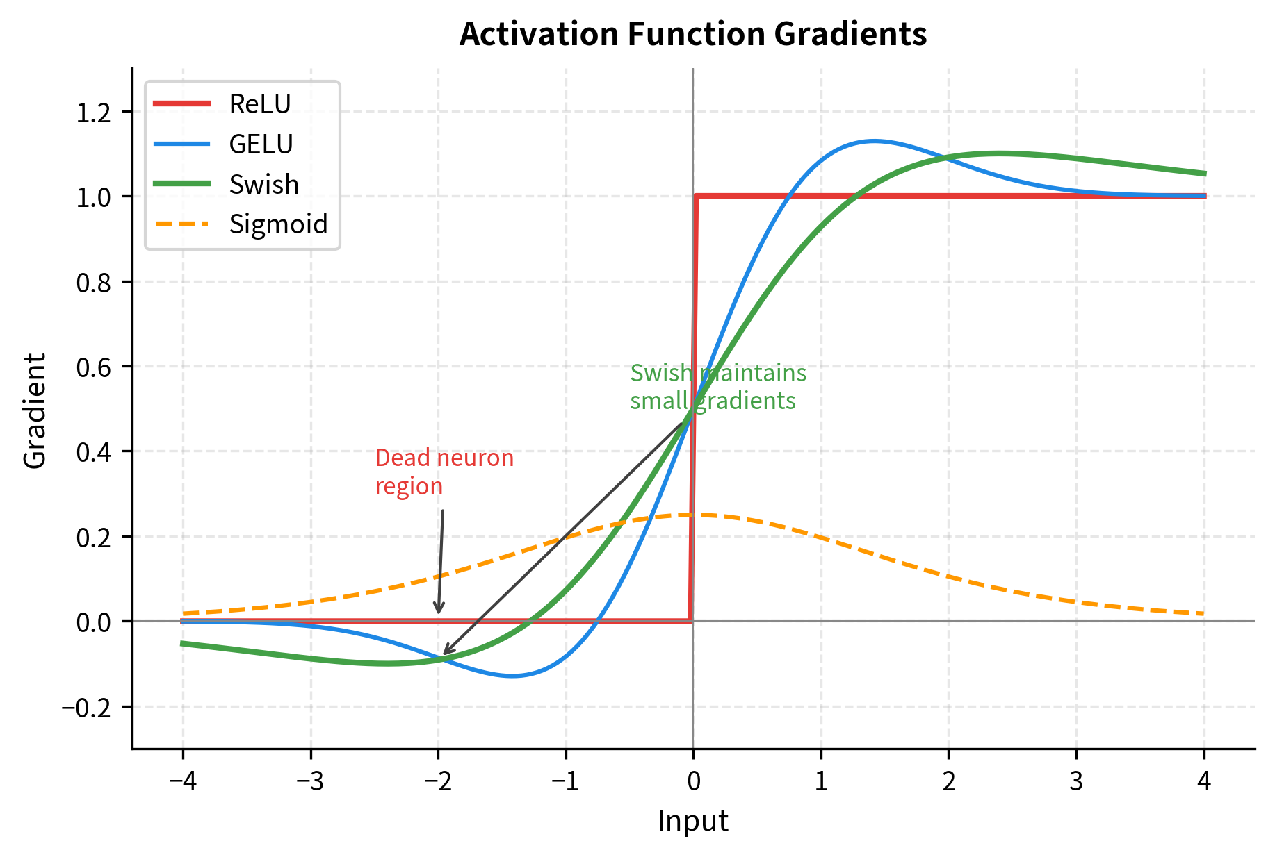
- Smooth gradients: Swish is differentiable everywhere with smooth gradients, avoiding the sharp transitions at zero that ReLU has
- Self-gating property: The formula means each dimension gates itself, creating input-dependent behavior without explicit gate parameters
- Better gradient flow: The linear term in Swish ensures gradients can flow even for extreme inputs, helping train deep networks
The gradient behavior is particularly important for training deep networks. Let's visualize how gradients flow differently through each activation:
Implementation
Let's implement SwiGLU and see these properties in action:
The output norm provides a rough measure of the magnitude of the transformation. With Xavier initialization, we expect the output norm to be similar to the input norm, indicating stable signal propagation through the network.
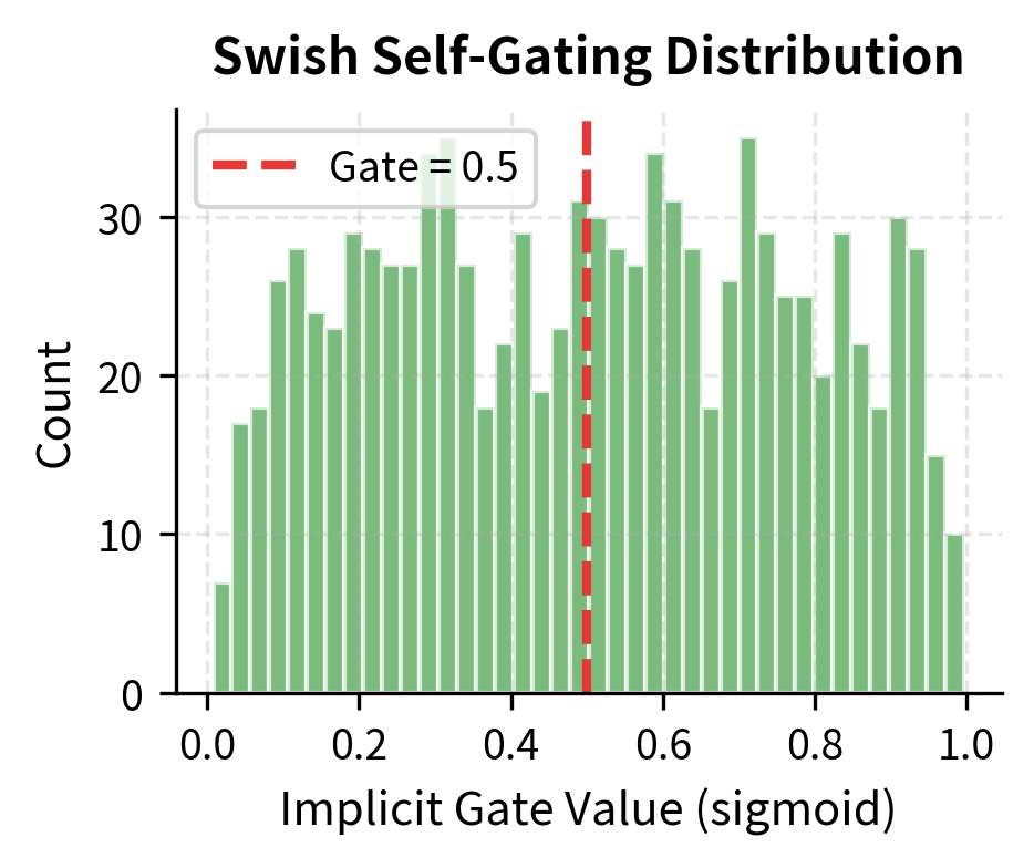
Let's examine the self-gating behavior of Swish more closely by looking at how the implicit gate values (the sigmoid component) distribute for random inputs:
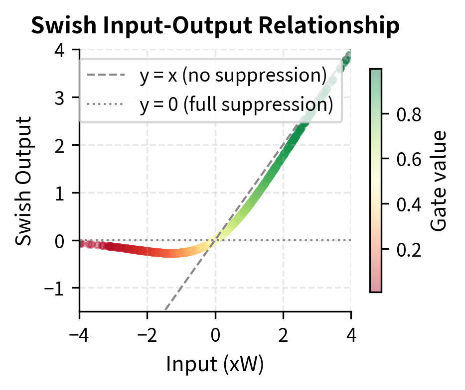
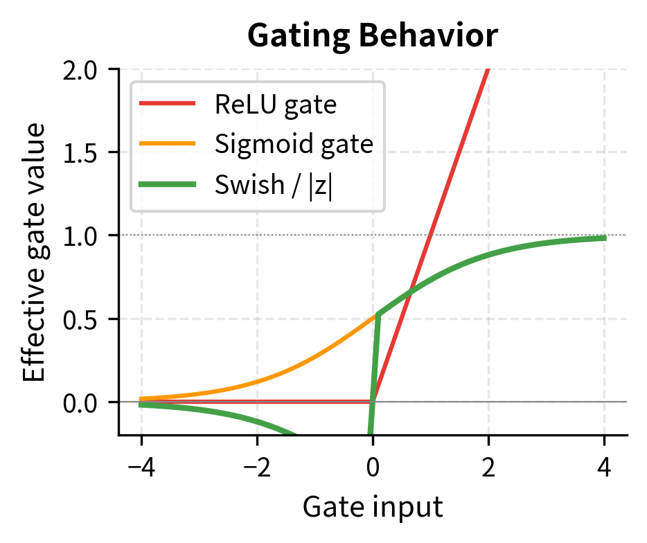
Let's also visualize how Swish compares to other activation functions and how this affects the gating behavior:
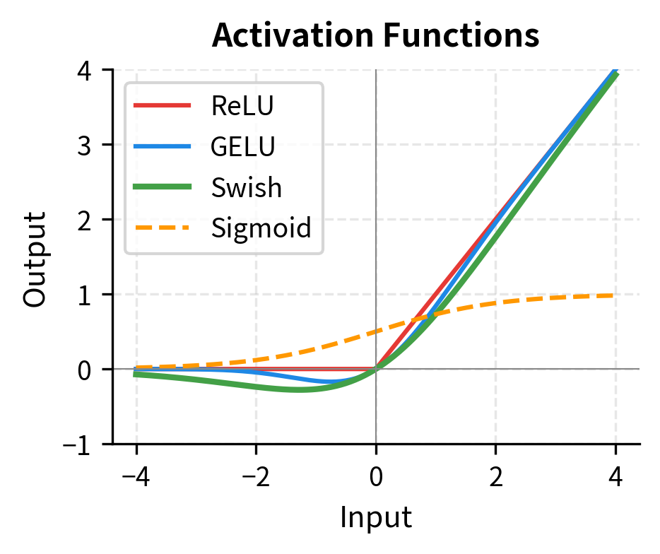
GeGLU: The GELU Variant
Another popular variant is GeGLU, which uses GELU instead of Swish for the gating function. The GeGLU formula follows the same pattern as SwiGLU, replacing the Swish activation with GELU:
where:
- : the input vector
- : the first projection matrix (GELU-activated pathway)
- : the second projection matrix (linear pathway)
- : element-wise multiplication (Hadamard product)
GELU (Gaussian Error Linear Unit) is defined as the product of the input and the cumulative distribution function (CDF) of the standard normal distribution:
where:
- : the input value (a scalar, applied element-wise to vectors)
- : the cumulative distribution function of the standard normal distribution, i.e., for
Computing the exact CDF is expensive, so in practice a fast approximation is used:
This approximation uses the hyperbolic tangent function to approximate the error function that underlies the normal CDF. The constant was empirically chosen to minimize approximation error across the typical input range.
GeGLU has similar properties to SwiGLU but with slightly different gradient characteristics. Some practitioners prefer GeGLU for encoder models (following BERT's use of GELU), while SwiGLU has become more common in decoder-only LLMs.
The output norms are similar between SwiGLU and GeGLU, indicating that both variants produce representations of comparable magnitude. The non-zero difference norm confirms that while the outputs are similar, they're not identical. These differences are subtle in terms of output statistics but can compound over many layers and matter for training dynamics and final model quality at scale.
Parameter Efficiency Analysis
A crucial consideration when adopting GLU variants is the parameter cost. The standard FFN has two weight matrices, while GLU-based FFNs have three. Let's analyze this trade-off carefully.
For a standard FFN with hidden dimension , the parameter count (ignoring biases) is:
This comes from two weight matrices:
- : parameters
- : parameters
For a GLU-based FFN with the same hidden dimension , the parameter count is:
This comes from three weight matrices:
- : parameters (value/Swish projection)
- : parameters (gate/linear projection)
- : parameters (output projection)
The GLU variant has 50% more parameters for the same hidden dimension. To maintain the same parameter count as a standard FFN, we can solve for the reduced hidden dimension :
Solving for :
This means we need to reduce by a factor of to match the parameter count of a standard FFN.
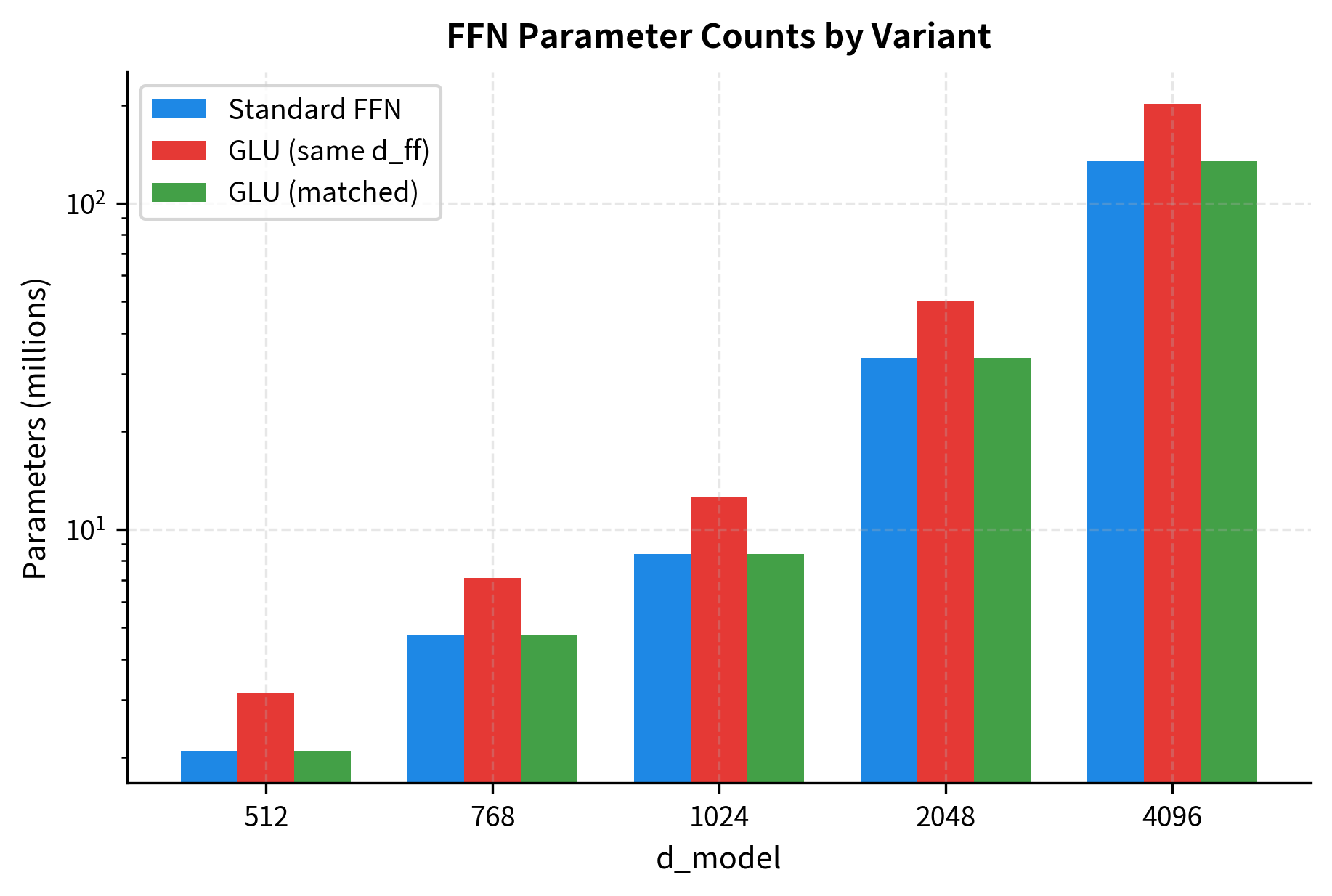
The comparison shows that keeping the same hidden dimension increases parameters by 50%, while reducing to 2048 brings the parameter count close to the standard FFN. This demonstrates the practical trade-off: you can either accept more parameters for the same hidden capacity, or reduce hidden capacity to match parameters while gaining the expressiveness of gating.
LLaMA and other modern models typically use the reduced hidden dimension approach. For example, LLaMA-7B uses with , which is approximately rather than the standard . This gives roughly the same parameter count as a standard FFN with expansion while gaining the benefits of gated activation.
Hidden Dimension Choices in Practice
Different models make different choices about how to handle the parameter trade-off. Let's examine the configurations used by several prominent models:
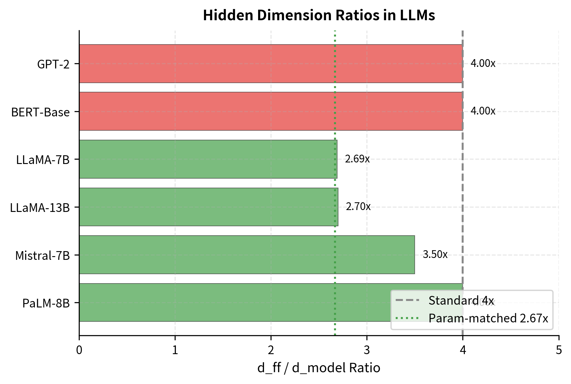
The table reveals interesting design choices across different models. Standard FFN models like GPT-2 and BERT use a consistent 4x ratio. SwiGLU models show more variation: LLaMA-7B uses 2.69x (close to parameter parity with 4x standard), while Mistral-7B and PaLM-8B use higher ratios, trading additional parameters for greater expressiveness.
Notice the pattern: models using SwiGLU tend to use ratios around 2.7x to 4x, depending on whether they prioritize matching the parameter count of standard FFNs or pushing expressiveness further. Mistral-7B, for example, uses a higher ratio (3.5x), accepting more parameters in exchange for potentially better quality.
Visualizing GLU Representations
To understand how GLU transforms representations differently from standard activations, let's visualize the hidden activations for the same inputs processed through different FFN variants:
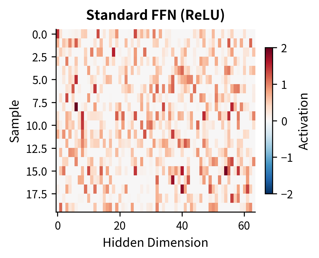
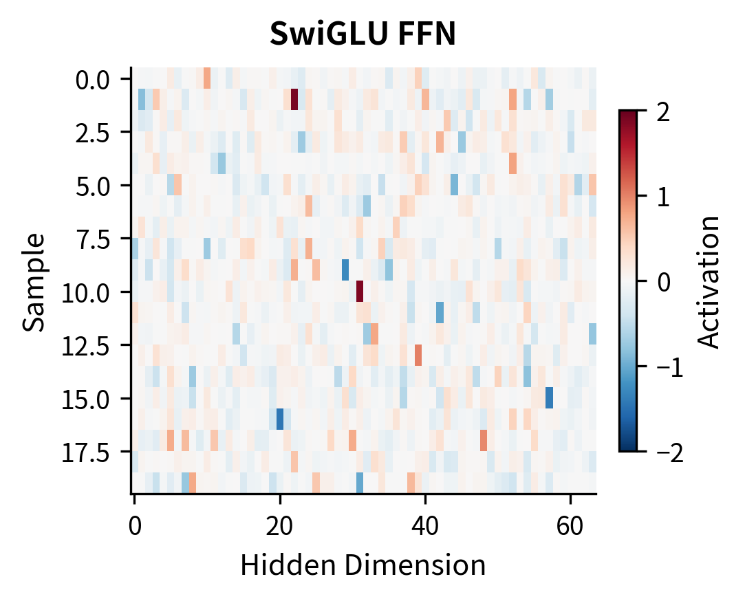
Let's also compare the distribution of activation values:
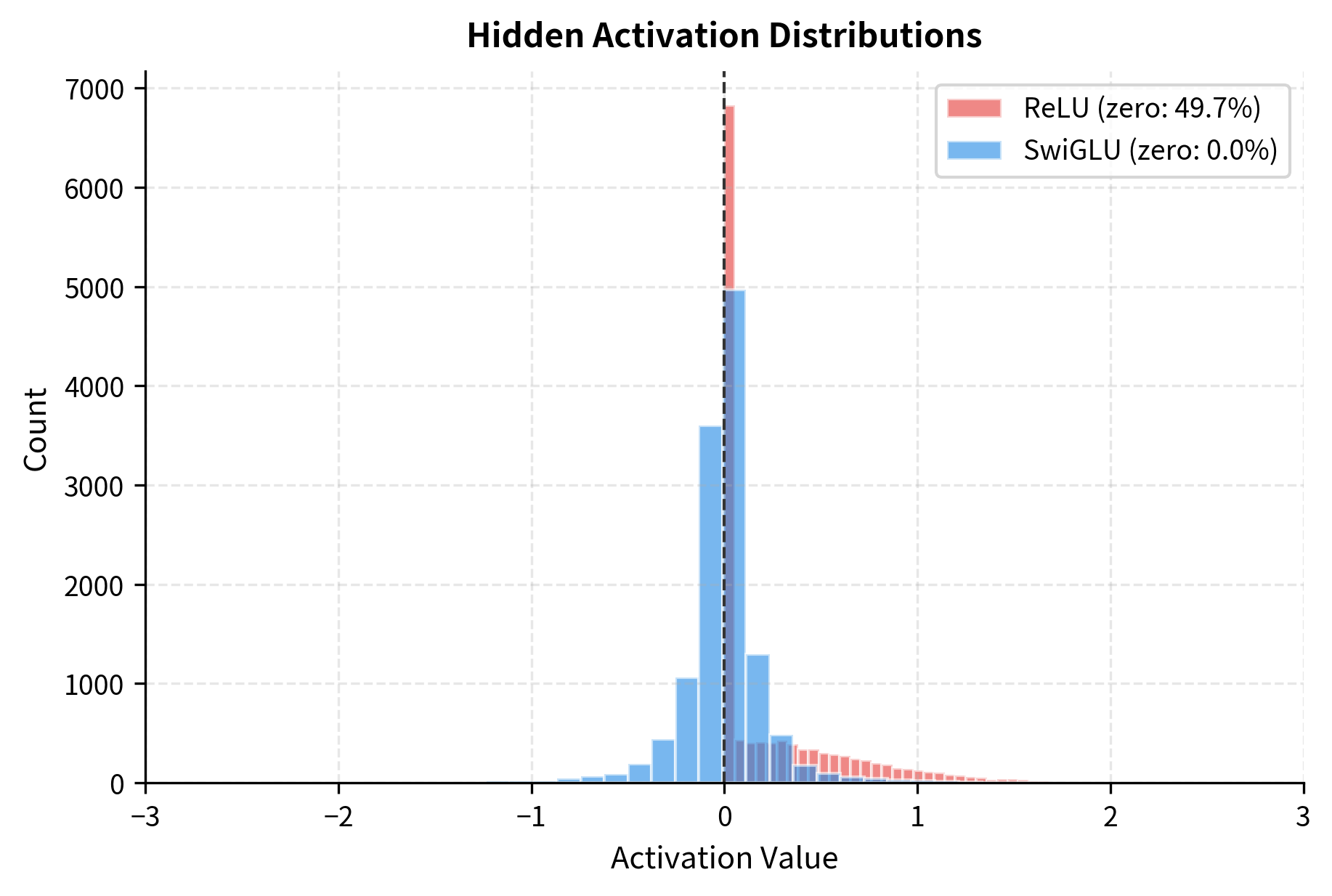
The key observation is that SwiGLU produces more continuous, less sparse activations. While ReLU creates hard sparsity (many exactly-zero values), SwiGLU allows for small negative values and smoother transitions. This can improve gradient flow during training and allows the network to represent more nuanced information.
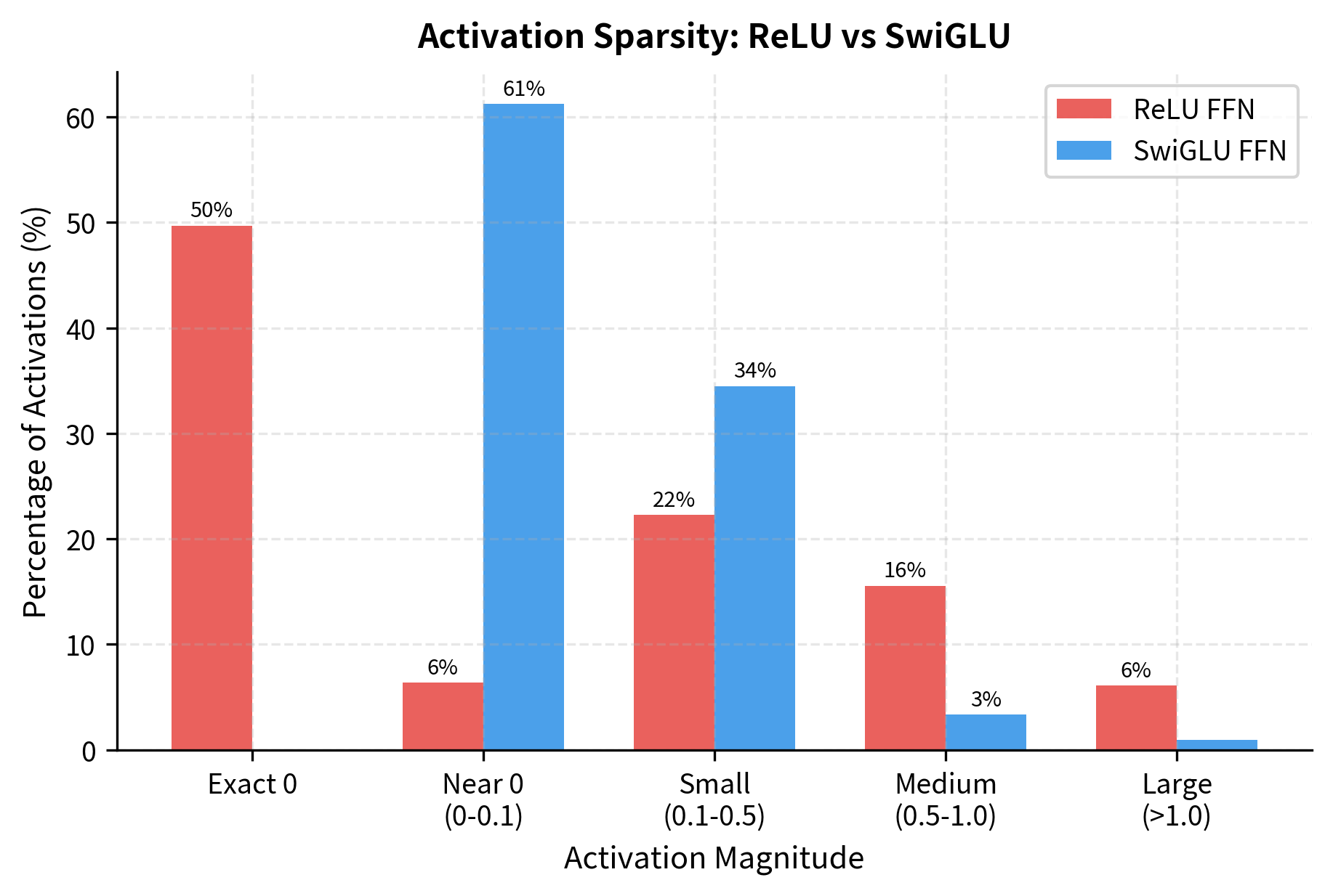
Let's quantify this sparsity difference more precisely by looking at how activation values distribute across magnitude ranges:
A Complete Worked Example
The formulas we've covered capture the essence of SwiGLU, but seeing actual numbers flow through the computation solidifies understanding. Let's trace through a concrete SwiGLU computation step by step, using deliberately small dimensions so you can follow every multiplication and understand exactly how the gating mechanism transforms an input vector.
Our goal is threefold:
We have a 4-dimensional input vector that we'll project into a 6-dimensional hidden space. The weight matrices and are initialized with small values for readability, and projects back from hidden to input dimension.
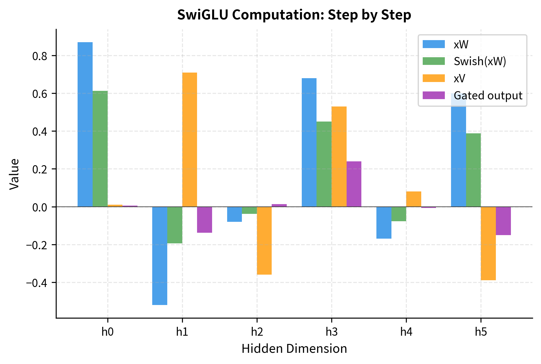
Now let's trace through each step of the SwiGLU computation:
The step-by-step output reveals several important patterns:
Step 1 vs Step 2 (Swish effect): Compare with . Notice how Swish preserves the sign but modulates the magnitude. Larger positive values shrink slightly (due to the sigmoid factor being less than 1 for small values), while negative values get pushed toward zero but can remain slightly negative (unlike ReLU which would zero them completely).
Step 3 (Linear pathway): The values in are independent from , giving the network a second "view" of the same input through different learned weights.
Step 4 (Multiplicative combination): The final hidden representation emerges from element-wise multiplication. When both pathways have the same sign, the product is positive; opposite signs yield negative products. Near-zero values in either pathway suppress that dimension in the output.
Let's visualize how each step transforms the representation:
Implementation: A Complete SwiGLU Module
Having traced through the mathematics by hand, we can now consolidate everything into a reusable implementation. This module follows the patterns used in production transformer libraries: it initializes weights using proper scaling (Xavier/Glorot initialization), supports optional biases, handles both single vectors and batched sequences, and provides a clean interface for integration into larger architectures.
The implementation below captures the complete SwiGLU FFN as used in LLaMA, Mistral, and other modern LLMs:
The SwiGLU module with reduced achieves comparable parameter count to a standard FFN with . The module correctly handles both single vectors and batched sequences, producing outputs of the expected shapes. This implementation follows the pattern used in production LLMs like LLaMA.
GLU in Modern Architectures
Gated Linear Units have become the de facto standard in modern large language models. Here's how different architectures implement GLU variants:
-
LLaMA (Meta, 2023): Uses SwiGLU with rounded to the nearest multiple of 256 for hardware efficiency. The rounding ensures tensor dimensions align well with GPU architectures. Biases are completely removed from the FFN.
-
Mistral (2023): Also uses SwiGLU but with a higher ratio (), trading parameters for expressiveness. Like LLaMA, no biases are used.
-
PaLM (Google, 2022): Uses SwiGLU with a 4x expansion ratio, accepting the higher parameter count in exchange for expressiveness. The model uses separate embedding and softmax matrices and applies RMS normalization.
-
Falcon (TII, 2023): Uses GELU rather than Swish in its GLU variant, following the BERT tradition while still benefiting from the gating mechanism.
Limitations and Impact
Gated Linear Units represent a significant improvement over standard feed-forward networks, but they come with trade-offs that practitioners should understand.
The primary limitation is computational overhead. While GLU variants match the parameter count of standard FFNs when using reduced hidden dimensions, they require three matrix multiplications instead of two (for , , and ). The element-wise multiplication between the two pathways adds minimal compute but requires storing both intermediate results, increasing memory pressure during training. On modern GPU hardware, this overhead is typically modest (10-15% additional compute), but it can matter for latency-critical applications or when operating near memory limits.
The reduced hidden dimension that maintains parameter parity also has implications. A standard FFN with provides 4x expansion before the nonlinearity. A SwiGLU FFN with matched parameters uses only expansion. While the gating mechanism compensates by providing richer interactions, some researchers hypothesize that very high expansion ratios may be beneficial for certain tasks, and GLU's parameter efficiency gains come at the cost of this expansion.
Despite these considerations, the impact of GLU on language model quality has been substantial. Empirical studies consistently show that SwiGLU improves perplexity and downstream task performance compared to standard FFNs with equivalent parameter counts. The improvement is robust across model scales, from small models with hundreds of millions of parameters to frontier models with hundreds of billions. This consistent benefit, combined with straightforward implementation, explains why virtually every state-of-the-art LLM released since 2022 uses some form of gated activation.
The gating mechanism also provides interpretability benefits. Researchers have found that individual dimensions in the gated hidden layer correspond more cleanly to semantic concepts than in standard FFNs. The gate values provide a natural measure of which features are "active" for a given input, enabling analysis techniques that probe what the model has learned. This interpretability, while not the primary motivation for GLU adoption, offers valuable tools for understanding model behavior.
Summary
Gated Linear Units transform the standard feed-forward network by introducing multiplicative interactions through learned gates. Rather than applying a simple activation function, GLU computes two parallel projections and multiplies them together, with one pathway controlling how much of the other passes through.
Key takeaways:
-
The gating mechanism: GLU computes , where is the input, and are learned projection matrices, is the sigmoid function producing gate values in , and denotes element-wise multiplication. This multiplicative interaction enables richer representations than additive transformations alone, capturing feature interactions that standard activations cannot express.
-
SwiGLU dominance: Modern LLMs predominantly use SwiGLU, defined as where is a self-gating activation that multiplies the input by its own sigmoid. The self-gating property of Swish, combined with the linear pathway, provides smooth gradients and unbounded positive outputs.
-
GeGLU alternative: GeGLU replaces Swish with GELU, offering similar benefits with slightly different gradient characteristics. It's sometimes preferred for encoder models following BERT's GELU tradition.
-
Parameter trade-offs: GLU requires three weight matrices (, , ) instead of two, adding 50% more parameters for the same hidden dimension. To maintain parameter parity, models reduce to approximately of the standard value. LLaMA uses instead of the standard .
-
Universal adoption: Since 2022, virtually every state-of-the-art LLM uses SwiGLU or a similar gated variant. LLaMA, Mistral, PaLM, and their derivatives all employ gated activations, demonstrating consistent improvements in perplexity and downstream tasks.
-
Smoother activations: Unlike ReLU's hard sparsity, SwiGLU produces smoother activation distributions with preserved negative values. This improves gradient flow during training and allows for more nuanced representations.
The next chapter examines how all the components we've covered, including residual connections, layer normalization, attention, and gated feed-forward networks, assemble into complete transformer blocks. We'll see how the ordering and connections of these elements create the powerful architecture that underlies modern language models.
Key Parameters
When implementing or configuring GLU-based feed-forward networks:
-
d_model (input/output dimension): The embedding dimension, unchanged from standard FFNs. Must match the attention layer output for proper residual connections.
-
d_ff (hidden dimension): The dimension of the gated intermediate representation. For parameter parity with standard FFNs, use . LLaMA rounds this to the nearest multiple of 256 for hardware efficiency. Higher ratios (3.5x or 4x) trade parameters for expressiveness.
-
glu_variant: The choice of activation function for gating. SwiGLU () is the dominant choice. GeGLU uses GELU instead. ReGLU uses ReLU but is less common due to ReLU's sharp transitions.
-
use_bias: Whether to include bias terms. Modern architectures (LLaMA, Mistral, PaLM) typically omit biases entirely, reducing parameters and simplifying quantization. The impact on model quality is minimal.
-
multiple_of (LLaMA-specific): Round to a multiple of this value (typically 256) for GPU memory alignment. The formula used is:
where is the multiple_of value and denotes the ceiling function. For example, with and : the raw value is , and rounding up to the nearest multiple of 256 gives .
Quiz
Ready to test your understanding? Take this quick quiz to reinforce what you've learned about Gated Linear Units and their role in modern language models.

Comments