
Learn why neural networks forget prior capabilities during fine-tuning and discover mitigation strategies like EWC, L2-SP regularization, and replay methods.

This article is part of the free-to-read Language AI Handbook
Choose your expertise level to adjust how many terms are explained. Beginners see more tooltips, experts see fewer to maintain reading flow. Hover over underlined terms for instant definitions.
Catastrophic Forgetting
When you fine-tune a pre-trained language model on a new task, something troubling happens: the model gets better at your task but worse at everything else. Train BERT on sentiment analysis, and it may forget how to perform named entity recognition. Fine-tune GPT on medical text, and it might lose fluency in general English. This phenomenon, known as catastrophic forgetting, represents one of the central challenges in adapting powerful pre-trained models to specific domains.
As we discussed in the Transfer Learning chapter, the entire premise of modern NLP rests on leveraging knowledge from pre-training. But that knowledge is fragile. Without careful management, fine-tuning doesn't augment a model's capabilities; it overwrites them. Understanding why forgetting occurs and how to mitigate it is essential for you when customizing models without destroying what made them useful in the first place.
The Forgetting Phenomenon
Catastrophic forgetting occurs when a neural network trained on a new task loses performance on previously learned tasks. Unlike human forgetting, which is gradual and often recoverable, neural network forgetting can be sudden and complete. A model might drop from 90% accuracy on a prior task to near-random performance after just a few epochs of fine-tuning on new data.
To understand why this happens, consider the fundamental difference between how humans and neural networks store knowledge. Human memory is distributed across biological structures that maintain some degree of modularity. When you learn to play piano, the neural pathways encoding your knowledge of how to ride a bicycle remain largely undisturbed. Neural networks, in contrast, encode all their knowledge in a single set of shared weights. Every capability the model possesses depends on the same pool of parameters, and any change to those parameters affects all capabilities simultaneously.
The tendency of neural networks to abruptly lose previously learned information when trained on new data, caused by weight updates that overwrite the representations responsible for earlier capabilities.
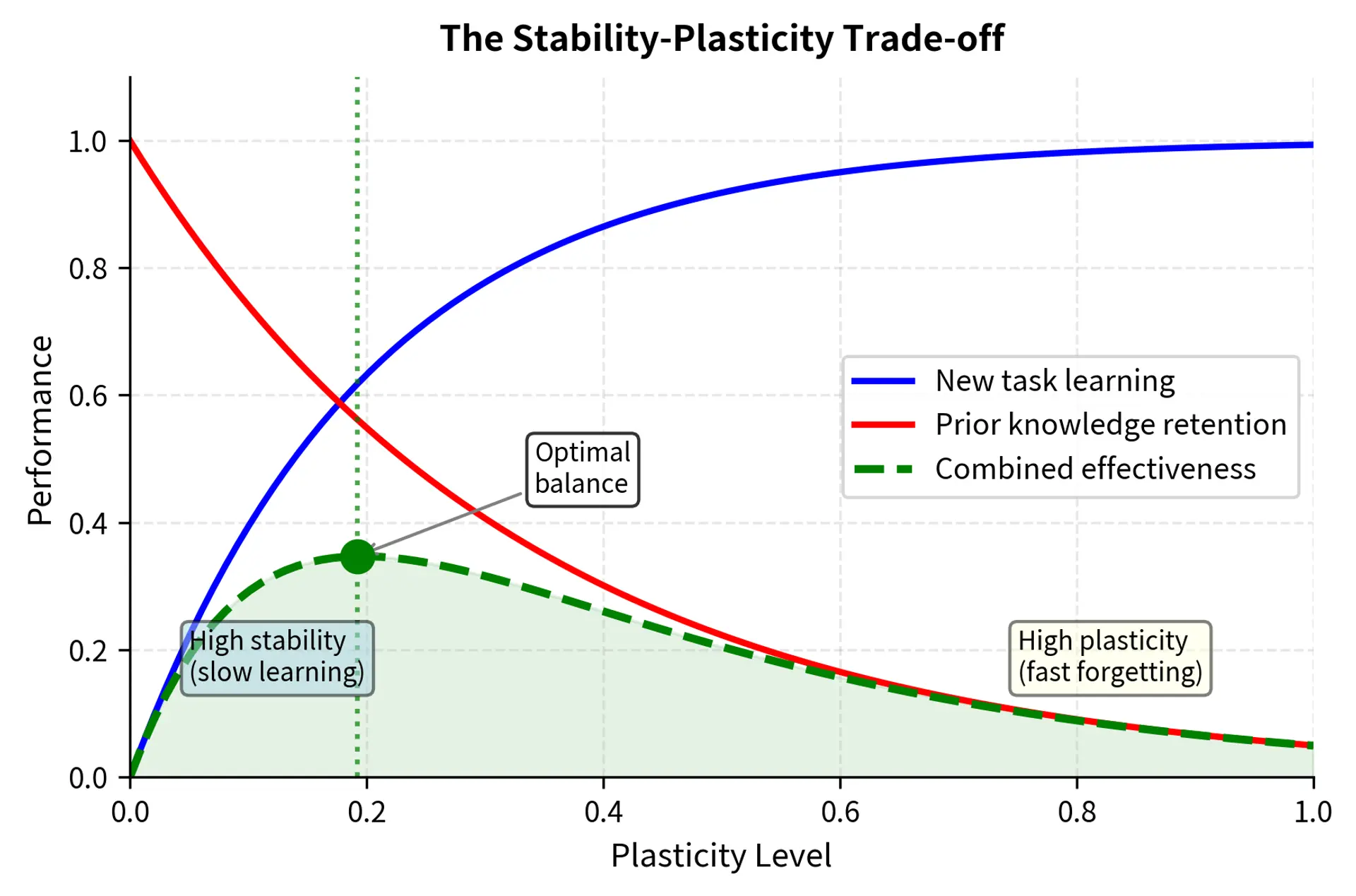
The Stability-Plasticity Dilemma
The root cause of catastrophic forgetting lies in a fundamental tension in learning systems: the stability-plasticity dilemma. This dilemma, first articulated in the neuroscience literature, captures an essential trade-off that any adaptive system must navigate. A learning system must be:
- Plastic enough to acquire new knowledge from incoming data
- Stable enough to retain previously learned information
These two requirements exist in fundamental tension. High plasticity allows rapid learning but makes existing knowledge vulnerable to being overwritten. High stability preserves existing knowledge but prevents the acquisition of new information. Biological brains have evolved sophisticated mechanisms to balance these competing demands, including separate memory systems for different timescales and consolidation processes that protect important memories. Neural networks, by design, are highly plastic. Each gradient update modifies weights throughout the entire network, with no built-in mechanism to distinguish between weights that should change and weights that must remain stable.
Consider what happens during fine-tuning. The loss function measures performance only on the new task. It provides no signal about whether the model still performs well on other tasks, because the training process simply does not observe performance on those tasks. Gradients flow backward through the network, and every parameter update asks a single question: "How can I better predict sentiment?" The network has no mechanism to simultaneously ask: "Will this change hurt my ability to recognize named entities?" or "Am I still generating grammatically correct English?" The optimization process is entirely myopic, focused exclusively on the current batch of fine-tuning data.
This myopia is not a flaw in the training algorithm. It is a direct consequence of the objective function we specify. Standard supervised learning optimizes performance on the training distribution, and nothing in that objective encourages preservation of capabilities that are not represented in the training data. The resulting forgetting is thus not a bug but an inevitable consequence of how we have defined the learning problem.
Why Pre-trained Knowledge is Vulnerable
Pre-trained language models learn rich representations that capture syntax, semantics, and world knowledge. These representations are distributed across millions or billions of parameters, with individual neurons participating in many different capabilities. This distributed nature is both a strength and a vulnerability. It is a strength because distributed representations enable powerful generalization and efficient parameter use. It is a vulnerability because any modification to the shared parameters can propagate to affect multiple capabilities, even those that seem unrelated to the task being fine-tuned.
During fine-tuning, several distinct mechanisms contribute to forgetting, each operating through different pathways but all leading to the same outcome: degradation of pre-trained capabilities.
Parameter drift occurs when weights shift away from their pre-trained values. Each gradient update nudges parameters in the direction that improves performance on the fine-tuning task. Individually, these nudges may seem small and harmless. But the effects accumulate across millions of parameters and thousands of gradient updates. Even small changes to individual weights, accumulated across millions of parameters, can dramatically alter the model's behavior on tasks not represented in the fine-tuning data. The model drifts through weight space, moving further and further from the region that supported its original capabilities.
Representational shift happens when the intermediate representations learned during pre-training are reorganized to better serve the fine-tuning task. During pre-training, the model learns to encode text into hidden states that capture general linguistic properties: part-of-speech information, semantic relationships, discourse structure, and more. During fine-tuning, these representations may be reshaped to emphasize features relevant to the new task while de-emphasizing features that are no longer useful. Hidden state distributions may shift in ways that break the assumptions of capabilities built on top of them. A downstream classifier trained to interpret the original hidden state space may receive inputs it cannot properly interpret when that space transforms.
Output distribution changes affect the final layers most severely. If pre-training encouraged a diverse vocabulary distribution, with the model learning to predict many different words in many different contexts, and fine-tuning focuses on domain-specific terms, the model may lose fluency with general vocabulary. The output layer's weights adapt to assign high probability to the words that appear frequently in the fine-tuning data, while the weights corresponding to rarely-seen words decay toward values that produce low probabilities.
Measuring Forgetting
To manage forgetting, we first need to quantify it. Without measurement, forgetting remains invisible until deployment reveals unexpected failures. Several metrics capture different aspects of how models deteriorate after fine-tuning, and choosing the right metric depends on what aspects of performance matter most for your application.
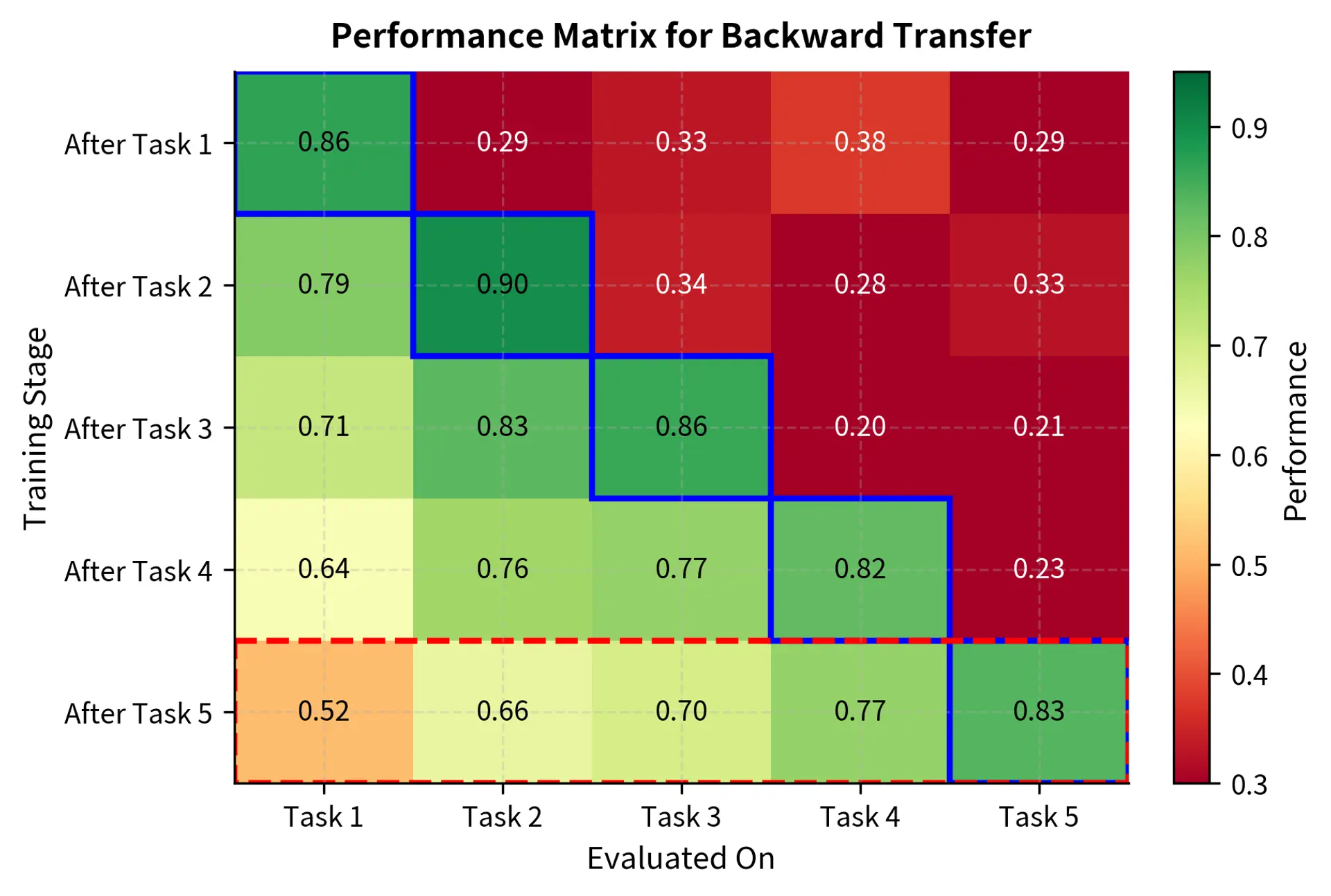
Backward Transfer
The most direct measure is backward transfer: how much does performance on prior tasks change after learning new ones? This metric captures the intuition that we want to compare the model's performance on old tasks before and after it learns something new. If the model performed well on named entity recognition before fine-tuning on sentiment analysis, backward transfer tells us how much of that NER performance survived.
To formalize this intuition, we need notation for tracking performance across multiple tasks learned sequentially. Imagine a model that learns task 1, then task 2, then task 3, and so on up to task T. At each point in this sequence, we can evaluate the model on any of the tasks it has encountered. The backward transfer metric computes the average change in performance across all previously learned tasks.
Let us unpack each component of this formula to understand exactly what it measures:
- : the backward transfer score, which summarizes how much prior task performance has changed
- : the total number of tasks learned sequentially, representing the full learning trajectory
- : the normalization term that computes the average change across all prior tasks, ensuring the metric is comparable regardless of how many tasks were learned
- : the performance on task after the model has finished training on all tasks, representing the model's current capability on that task
- : the baseline performance on task immediately after it was originally learned, representing the best performance the model achieved when that task was its primary focus
- : the summation over all previous tasks (excluding the current final task ), accumulating the performance changes across the model's learning history
The intuition behind this formula is straightforward: for each prior task, we compute how much performance changed from immediately after learning that task to the present moment, then average these changes. Negative backward transfer indicates forgetting, as it means current performance is lower than initial performance. A model with backward transfer of -0.15, for instance, has lost an average of 15 percentage points on prior tasks. Positive backward transfer would indicate that learning new tasks somehow improved performance on old tasks, a phenomenon called positive transfer that can occur when tasks share structure.
Forgetting Measure
A related metric tracks the maximum performance achieved on each task versus current performance. This metric addresses a subtle limitation of backward transfer: what if performance on a task fluctuates during training? Perhaps the model's NER performance actually increased slightly after learning sentiment analysis, before crashing when a third task was learned. The forgetting measure captures the worst-case degradation from peak performance.
Understanding each term in this formula reveals how it differs from backward transfer:
- : the forgetting measure for a specific task , quantifying how much performance on that particular task has degraded from its peak
- : the highest performance recorded for task at any previous time step , representing the best the model ever did on this task throughout its training history
- : the performance on task after training on task , allowing us to track performance at each point in the training sequence
- : the current performance on task after training on the final task , representing where the model stands now
This captures how much performance has degraded from the best observed level, regardless of when that peak occurred. A task might achieve peak performance not immediately after being learned, but at some later point when a related task was trained. The forgetting measure accounts for this by always comparing against the best-ever performance, providing a more comprehensive picture of capability loss.
Perplexity Degradation
For language models, perplexity on held-out general text provides a task-agnostic forgetting measure. Perplexity quantifies how surprised the model is by text it has not seen before. Lower perplexity indicates better language modeling capability, as the model assigns higher probability to the actual words that appear.
If a model's perplexity on Wikipedia increases from 15 to 45 after fine-tuning on legal documents, that quantifies how much general language modeling capability was lost. The model has become three times more surprised by general English text, indicating substantial degradation in its ability to model the distribution of ordinary language. This metric is particularly valuable because it does not require defining specific tasks. It measures the model's overall competence with language rather than its performance on any particular downstream application.
Benchmark Suites
In practice, we use standardized benchmark suites to measure forgetting comprehensively. These suites provide a battery of diverse tasks that together assess the breadth of a model's capabilities. For encoder models like BERT, the GLUE benchmark provides multiple tasks spanning sentiment analysis, textual entailment, and semantic similarity. Performance across this suite reveals whether fine-tuning has preserved the model's general language understanding or degraded it.
For generative models, evaluations might include:
- Language modeling perplexity on diverse corpora
- Zero-shot performance on reasoning benchmarks
- Few-shot classification accuracy
- Generation quality metrics (fluency, coherence)
These comprehensive evaluations provide a multidimensional view of forgetting, revealing which capabilities survived fine-tuning and which did not.
Visualizing Forgetting Dynamics
Let's examine how forgetting manifests during fine-tuning. We'll simulate a simplified scenario to build intuition.
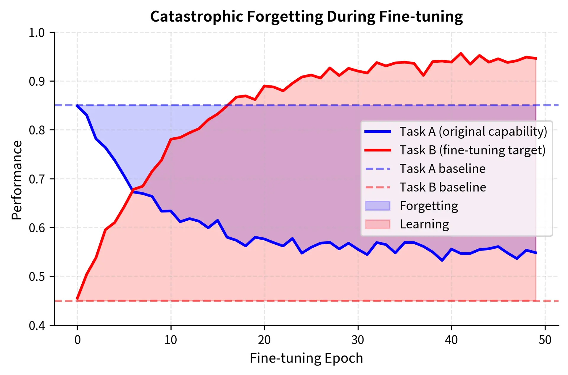
The visualization reveals a characteristic pattern: most forgetting happens early in training when learning rates are highest and the model is adjusting most aggressively. Later epochs show diminishing returns on both learning and forgetting as the model approaches a new equilibrium.
Causes at the Parameter Level
To understand forgetting deeply, we need to examine what happens to individual parameters during fine-tuning. The aggregate measures of forgetting we discussed earlier emerge from microscopic changes happening simultaneously across millions of weights. By understanding these parameter-level dynamics, we can design more targeted interventions.
Weight Importance Varies
Not all parameters contribute equally to each task. Some weights are critical for general language understanding, carrying information about syntax and semantics that applies broadly. Others specialize in specific capabilities, encoding task-specific patterns that are only relevant in certain contexts. Many are relatively unimportant for any particular function, serving as "slack" capacity that the model uses flexibly.
The challenge is that fine-tuning doesn't distinguish between these categories; it updates all parameters to reduce the fine-tuning loss. The gradient provides information about how changing each parameter would affect the fine-tuning objective, but it provides no information about how those same changes would affect other objectives. A parameter critical for named entity recognition receives the same treatment as a parameter that is entirely unimportant for prior capabilities.
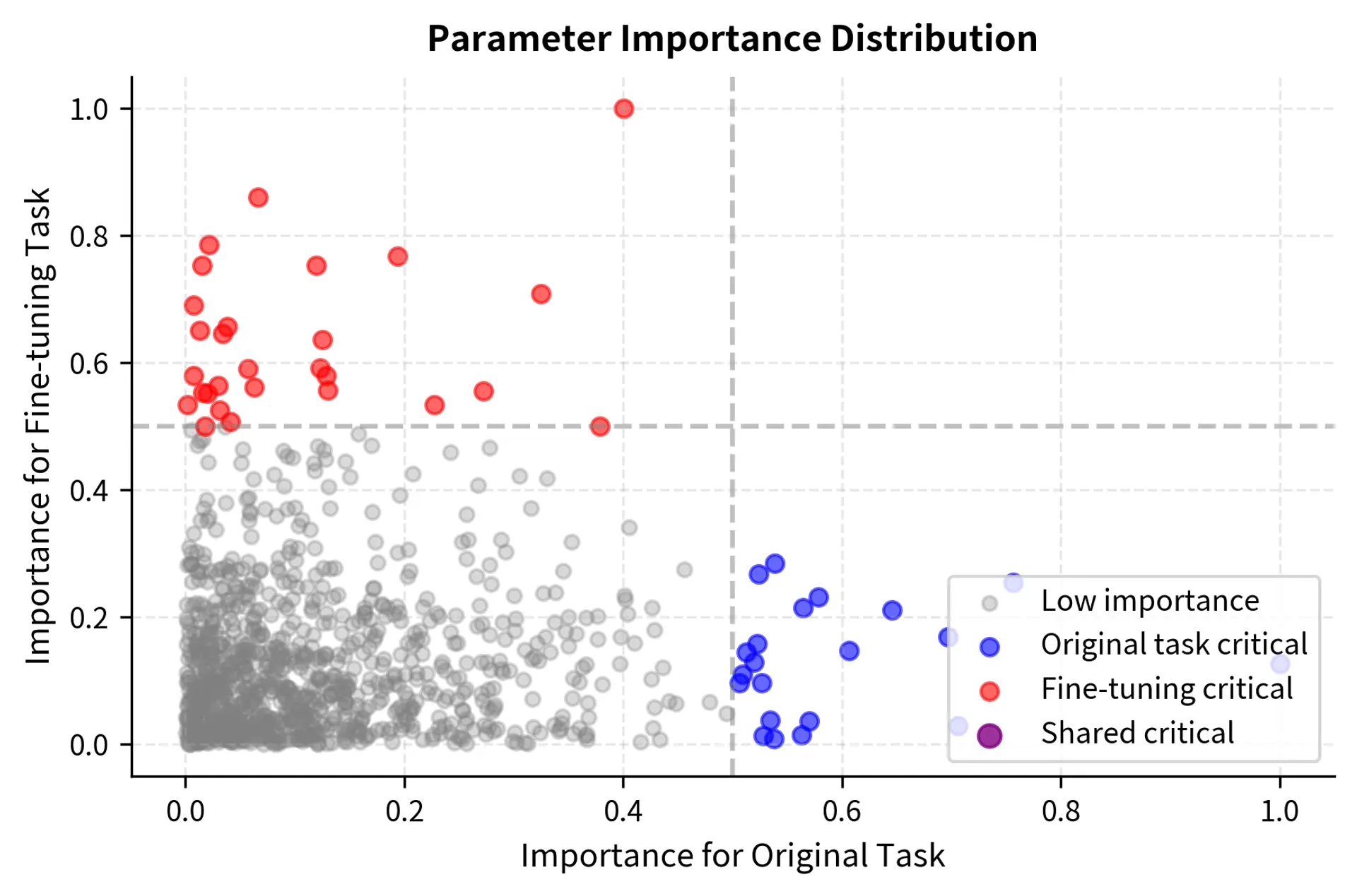
The key insight is that parameters in the "original task critical" category (blue points) need protection during fine-tuning. If these weights change significantly, original capabilities degrade, even if the changes help the fine-tuning objective. The scatter plot reveals the geometry of this problem: parameters occupy different regions depending on their importance to each task, and the region that matters most for forgetting is the one containing parameters that are important for original capabilities but not for the fine-tuning task.
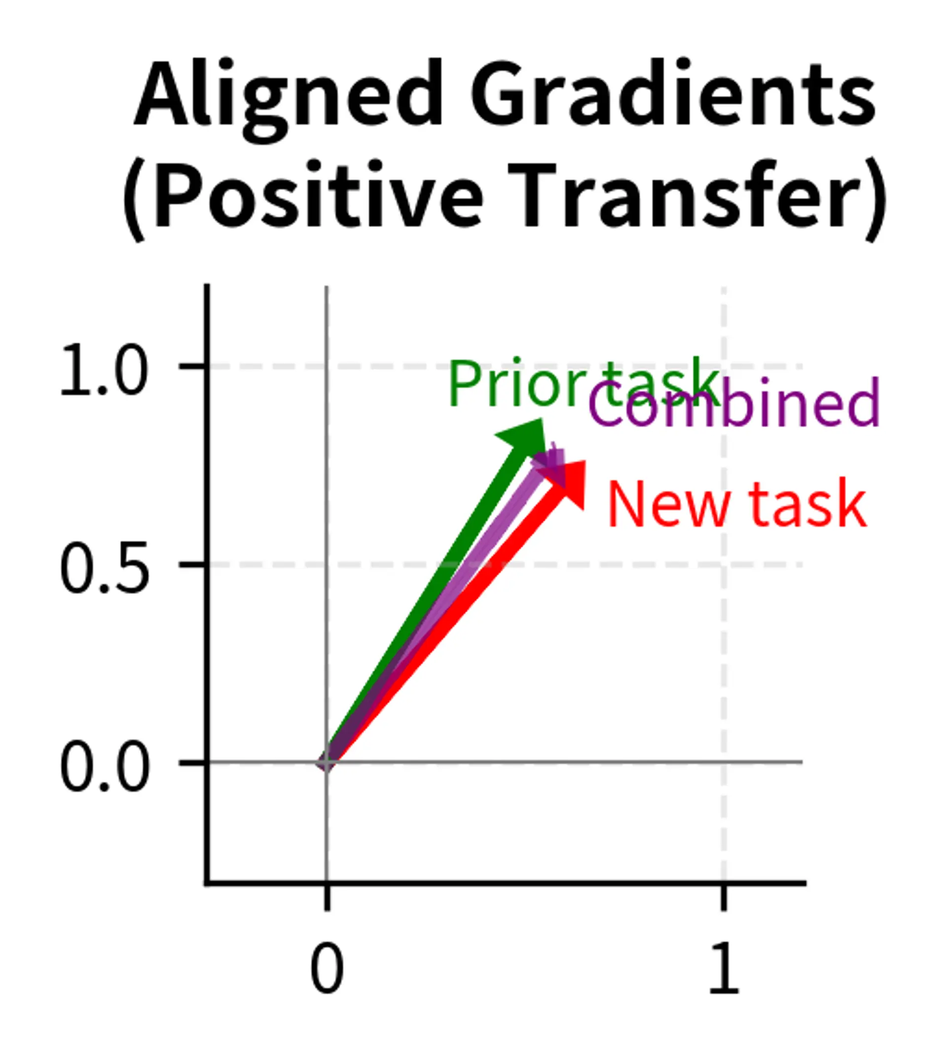
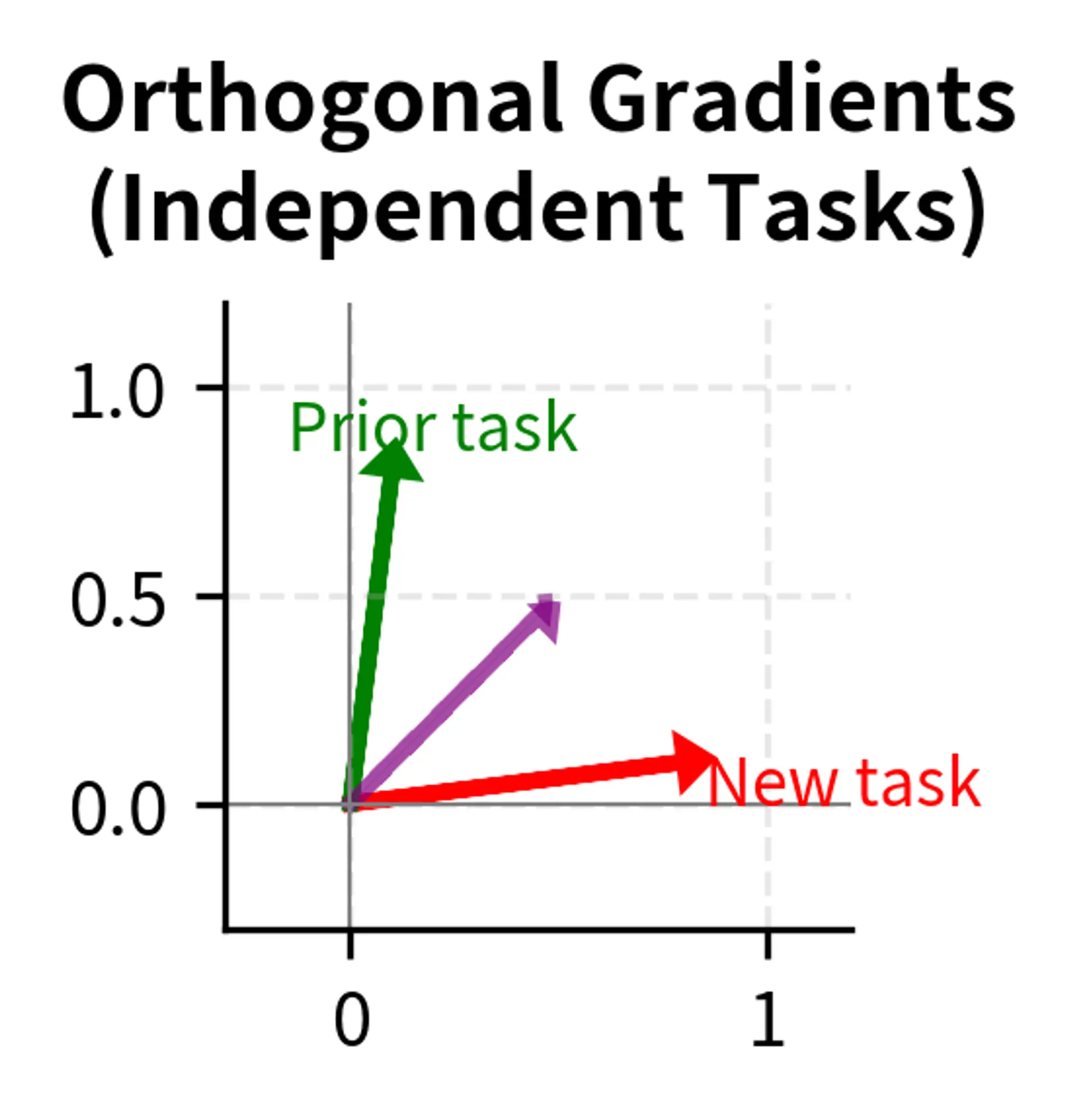
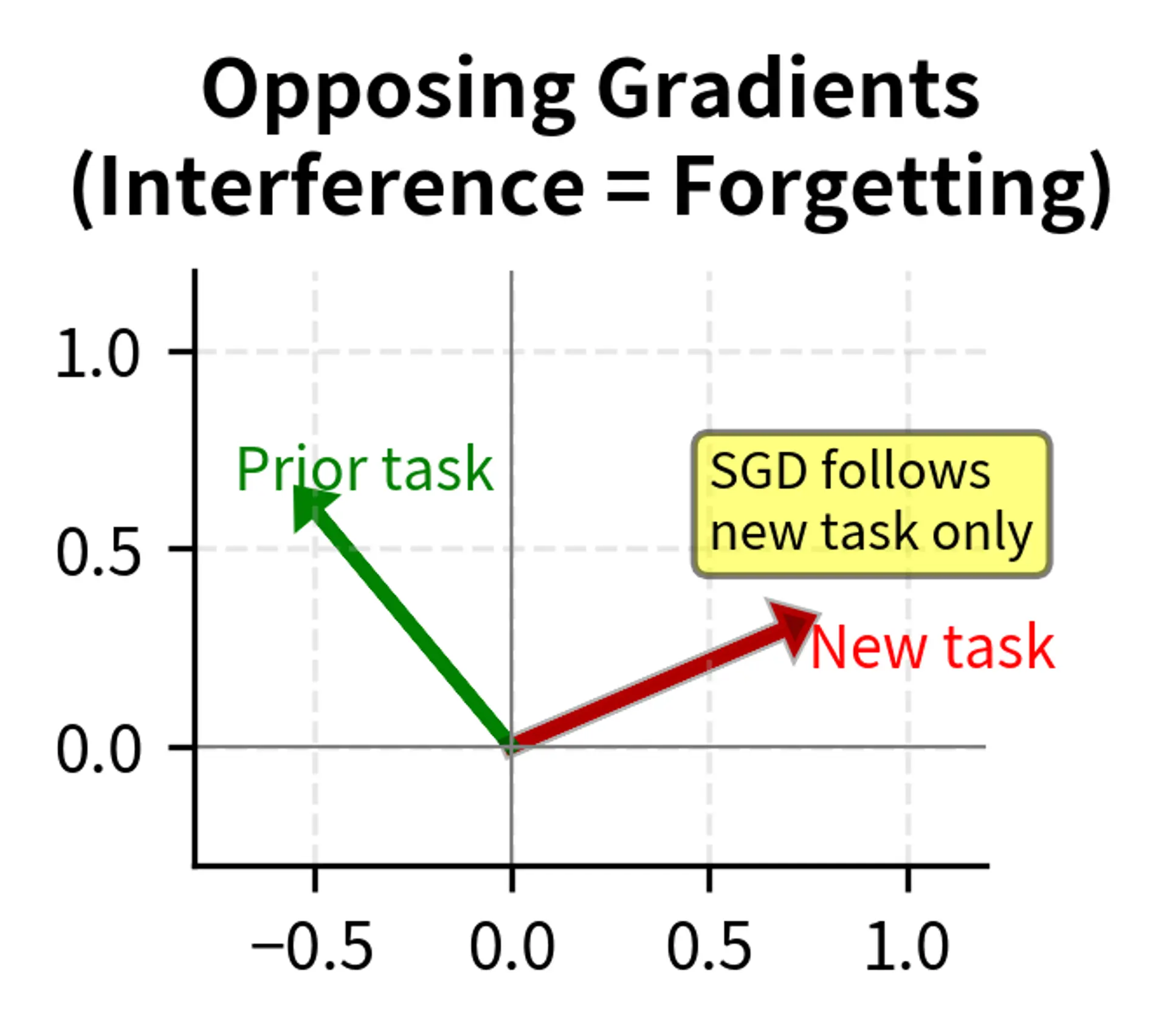
Gradient Interference
When gradients for the fine-tuning task oppose what would maintain original capabilities, we have gradient interference. This phenomenon occurs when the direction that improves the fine-tuning objective is exactly opposite to the direction that would preserve prior performance.
Consider a weight that needs to increase to improve sentiment classification but whose original value supported named entity recognition. Standard gradient descent simply follows the fine-tuning gradient, potentially destroying NER performance. The optimizer has no way to know that this particular weight is important for a capability we want to preserve. It only sees the gradient pointing upward and dutifully moves the weight in that direction.
Gradient interference is particularly insidious because it is invisible during training. The training loss decreases, validation accuracy on the fine-tuning task improves, and everything appears to be working correctly. Only when we evaluate on prior tasks do we discover that the gradients we followed led us away from the region of weight space that supported those capabilities.
Forgetting Mitigation Strategies
We have developed numerous techniques to reduce forgetting. These fall into several broad categories.
Regularization-Based Methods
These approaches add terms to the loss function that penalize changes to important parameters. The key insight behind regularization methods is that we can encode our desire to preserve prior capabilities directly into the objective function. By adding a penalty for parameter drift, we change the optimization landscape so that the model must balance improving on the new task against staying close to its original weights.
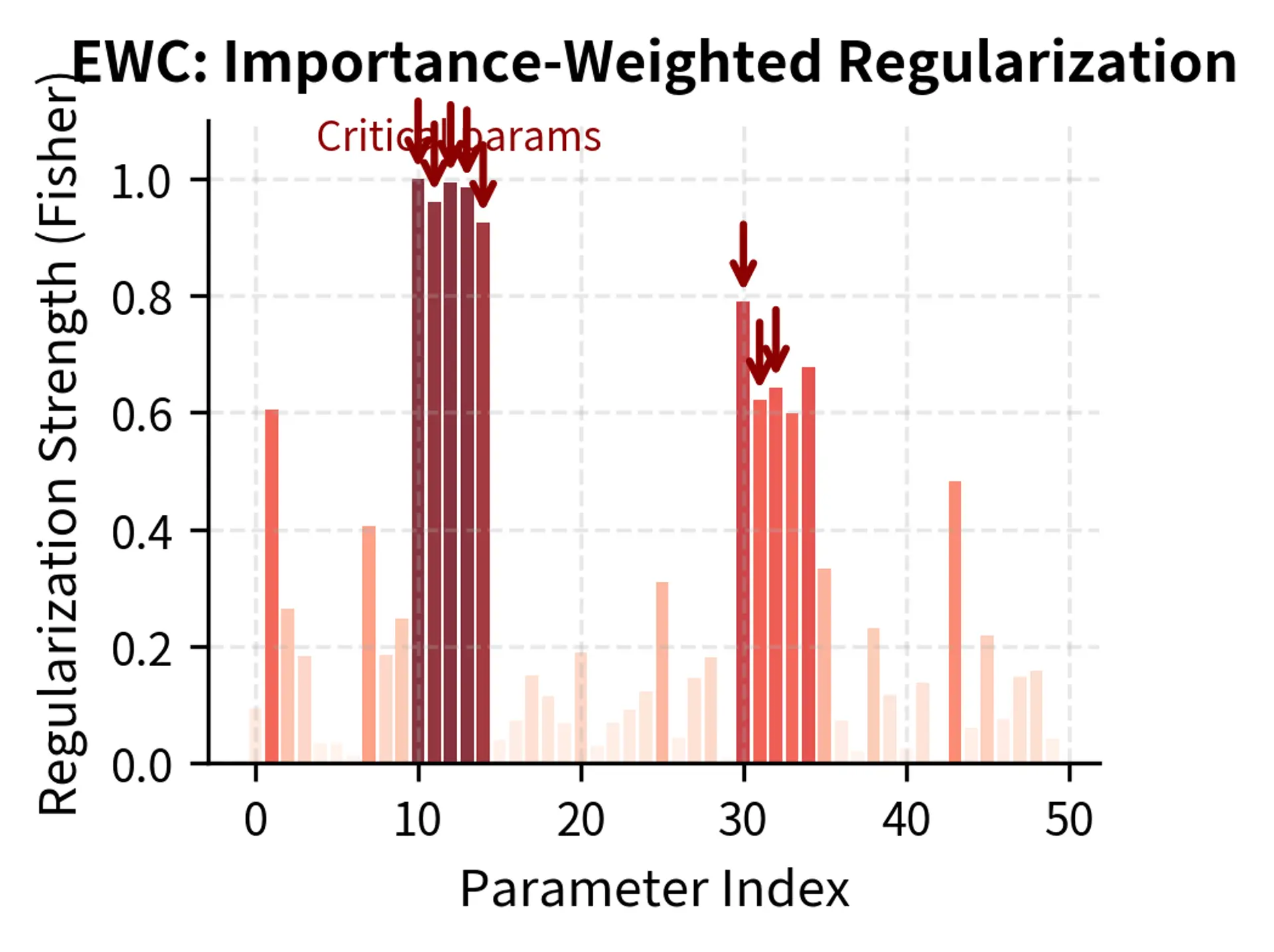
Elastic Weight Consolidation (EWC) identifies parameters important to prior tasks using the Fisher information matrix, then adds a penalty for changing those parameters. The Fisher information matrix provides a principled way to estimate parameter importance: parameters with high Fisher information are those where small changes cause large changes in the model's predictions on prior tasks. By penalizing changes to these high-importance parameters more heavily than changes to low-importance parameters, EWC implements a form of selective protection.
The EWC loss function combines the standard task loss with a weighted regularization term:
Understanding each component of this formula reveals the mechanism by which EWC prevents forgetting:
- : the composite loss function used during fine-tuning, which the optimizer minimizes
- : the standard loss function (e.g., cross-entropy) for the new task, ensuring the model still learns the fine-tuning objective
- : a hyperparameter controlling the regularization strength, allowing you to trade off between task performance and capability preservation
- : the Fisher information value for parameter , representing its importance to the previous task by approximating the curvature of the loss surface near the current parameter values
- : the current value of parameter during training, which changes as optimization proceeds
- : the value of parameter in the pre-trained (original) model, serving as the anchor point that regularization pulls toward
- : the summation over all parameters in the neural network, ensuring every weight is subject to regularization
The key innovation in EWC is the use of Fisher information to weight the regularization. Parameters with high Fisher information, those whose changes would strongly affect predictions on prior tasks, receive stronger protection. Parameters with low Fisher information can change more freely to accommodate the new task. This selective protection allows the model to adapt where it can and stay stable where it must.
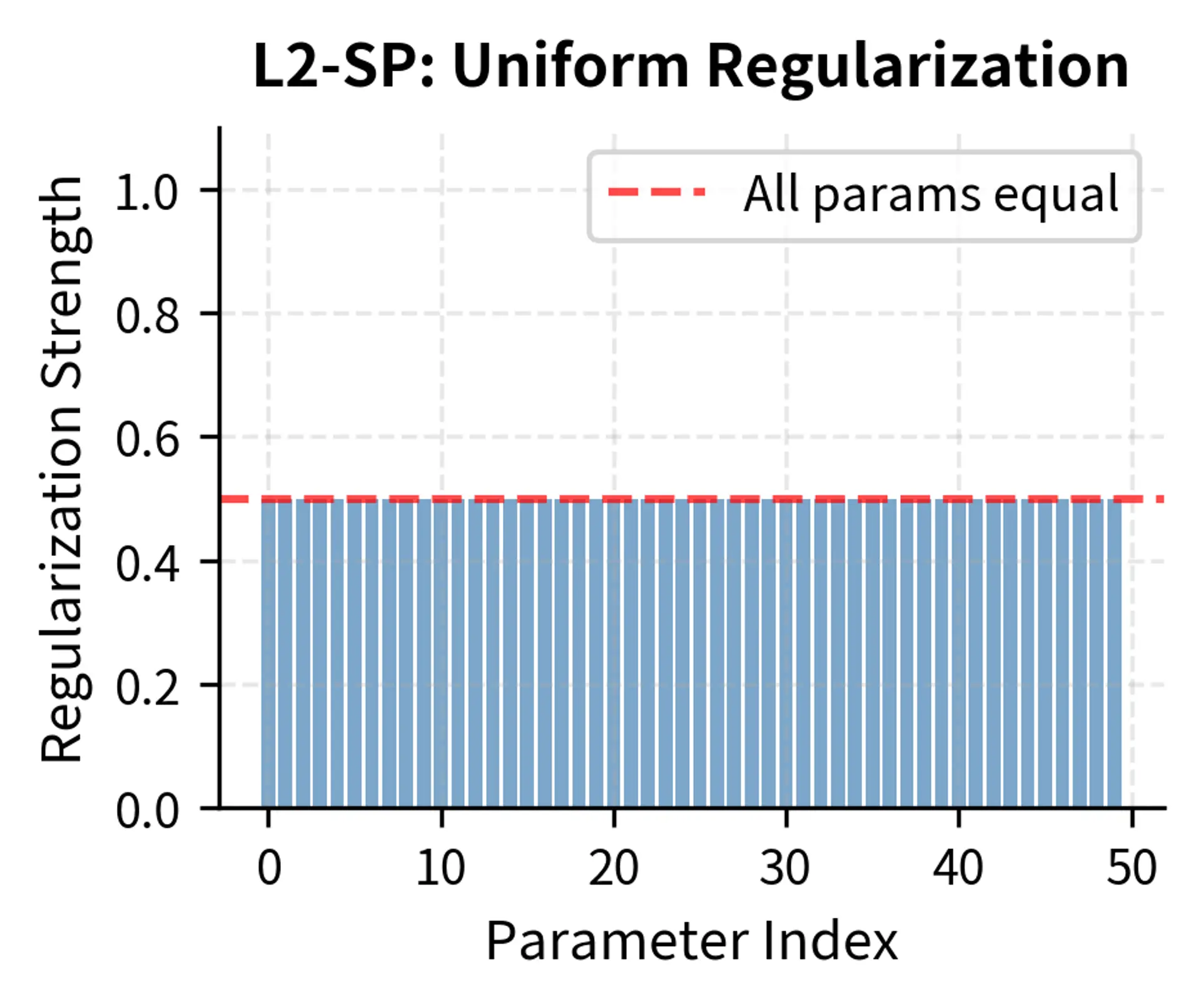
L2 regularization toward pre-trained weights is a simpler variant that penalizes all parameter changes equally. Rather than estimating parameter importance through Fisher information, L2-SP (L2 to Starting Point) assumes all parameters are equally important. This simplification dramatically reduces computational overhead while still providing meaningful protection against drift.
Breaking down this formula shows how it implements uniform regularization:
- : the regularized loss function (L2-SP stands for "L2 to Starting Point"), representing the objective the optimizer minimizes
- : the loss for the current fine-tuning task, ensuring the model still learns to perform the new task well
- : the regularization strength hyperparameter, controlling how strongly the model is pulled back toward its original weights
- : the current value of parameter during training
- : the value of parameter in the pre-trained (original) model
- : the sum of squared differences between current parameters and pre-trained parameters, measuring total drift from the original model
This formulation is equivalent to EWC if we assume every parameter has equal importance (i.e., for all ). It prevents the model parameters from drifting too far from their starting values, treating all weights as equally critical. While this uniform treatment is less sophisticated than EWC's selective protection, it often works surprisingly well in practice and requires no additional computation to estimate parameter importance.
Replay-Based Methods
Replay methods maintain performance on prior tasks by mixing in examples from previous training:
- Experience replay stores a subset of pre-training examples and includes them in each fine-tuning batch. This ensures the model continuously sees data from the original distribution.
- Generative replay uses the model itself (or a separate generator) to produce synthetic examples resembling pre-training data, avoiding the need to store actual training examples.
Architecture-Based Methods
Rather than regularizing training, architecture approaches modify the model structure:
- Progressive networks add new capacity for each task while freezing previous parameters entirely. This eliminates forgetting but dramatically increases model size.
- Adapter layers insert small trainable modules while keeping pre-trained weights frozen. We'll explore this approach in detail in the upcoming chapters on parameter-efficient fine-tuning (PEFT).
Learning Rate Strategies
Careful learning rate management significantly impacts forgetting:
- Discriminative learning rates apply smaller learning rates to earlier layers (which encode more general features) and larger rates to later layers (which are more task-specific).
- Learning rate warmup starts with very small updates, allowing the model to find a gentle path toward the fine-tuning objective without abrupt changes.
- Early stopping based on validation performance on both the fine-tuning task and held-out prior tasks can prevent excessive forgetting.
Implementing Forgetting Measurement
Let's implement a practical framework for measuring forgetting during fine-tuning. We'll use a sentiment classification task while monitoring language modeling capability.
Now let's run fine-tuning while tracking both task performance and general capability:
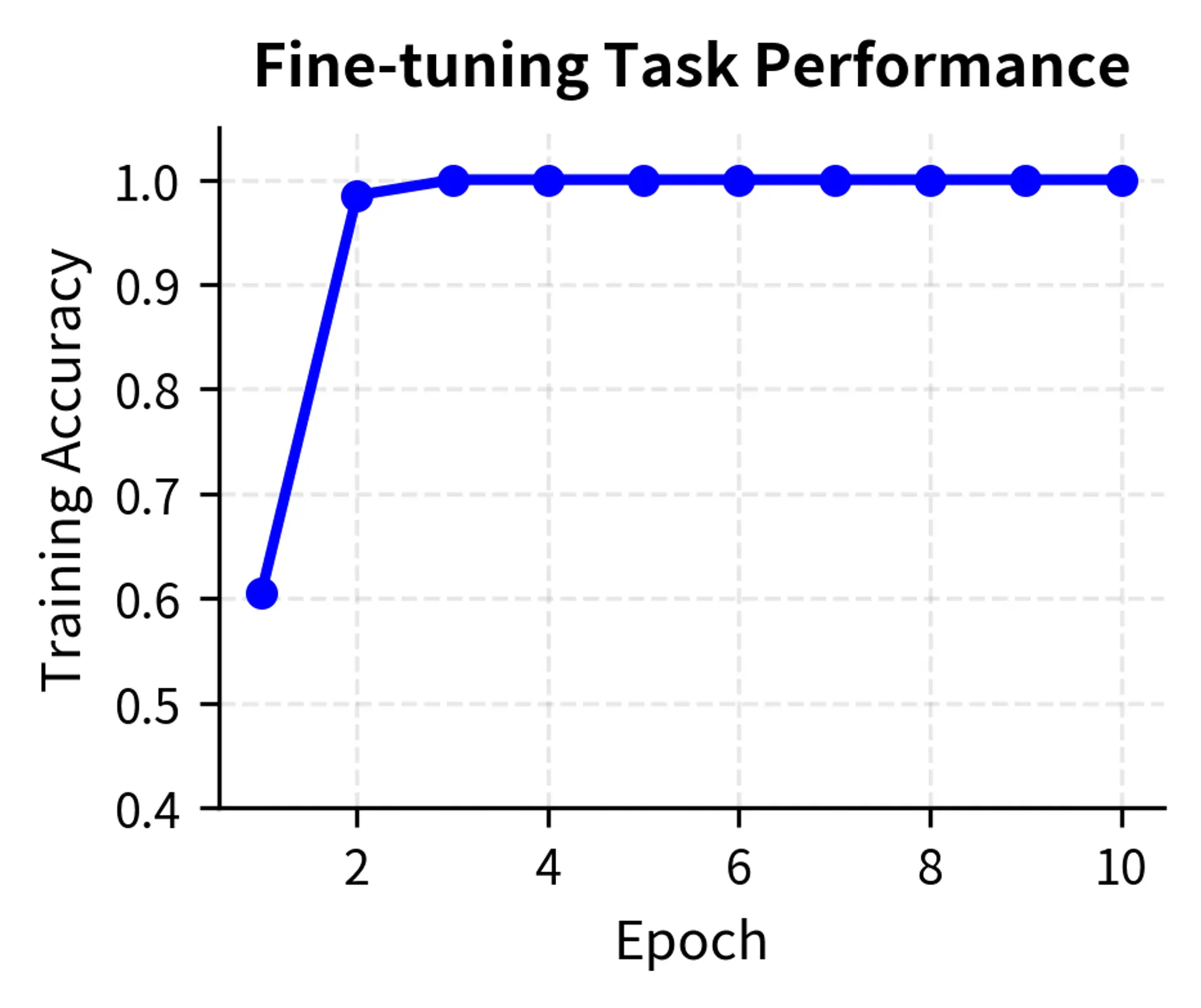
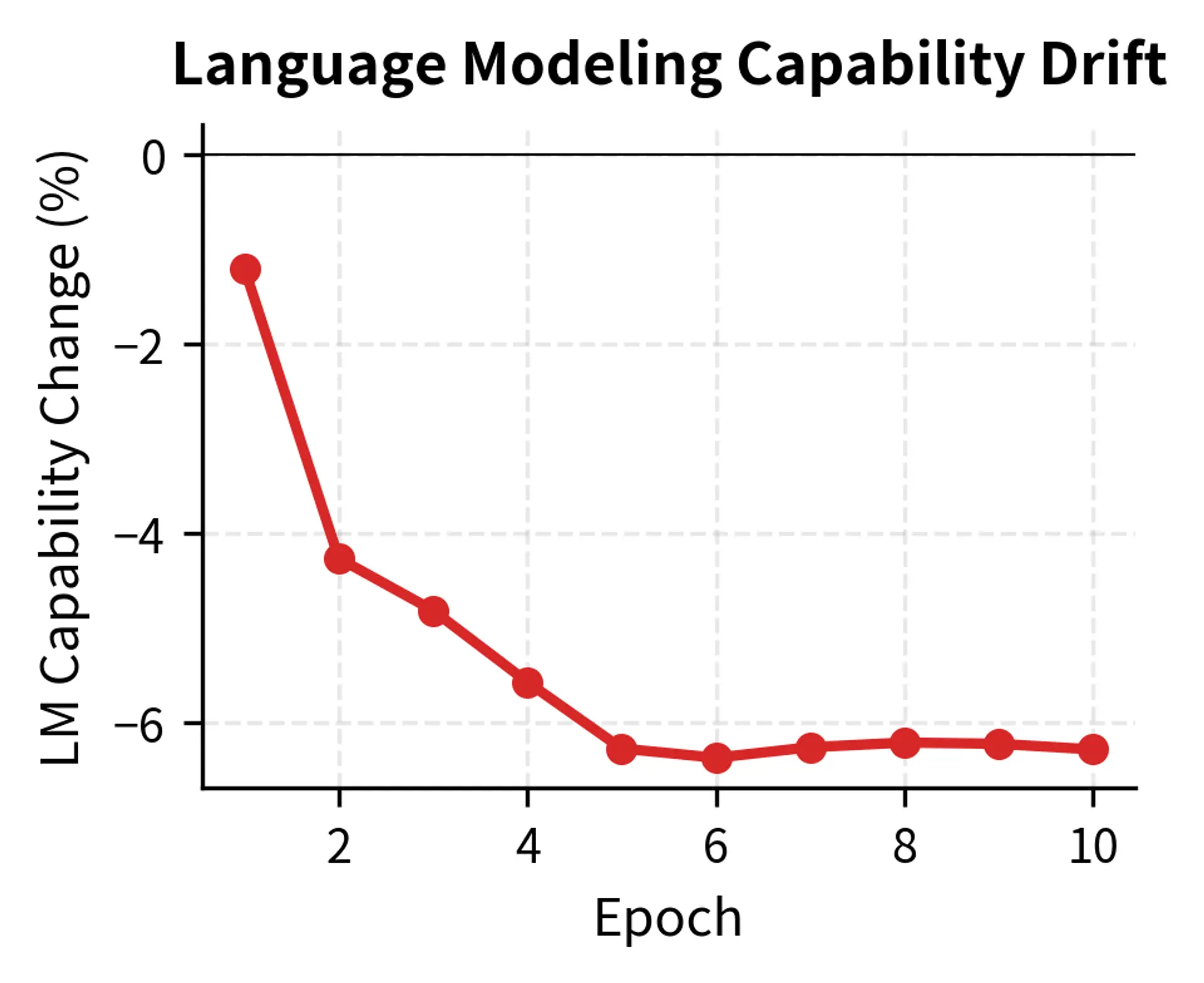
The divergence between task accuracy and language modeling capability quantifies the severity of forgetting. While the model masters the sentiment task, the negative LM score change indicates a degradation in general linguistic competence, a warning sign for deployment.
Implementing L2-SP Regularization
Let's implement L2-SP (L2 regularization toward Starting Point), a simple but effective forgetting mitigation technique:
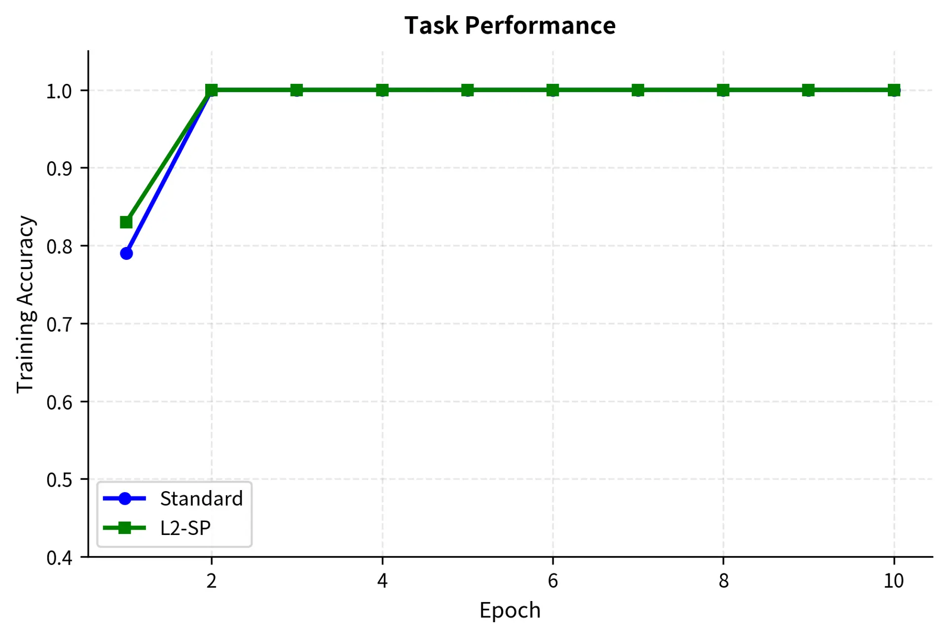
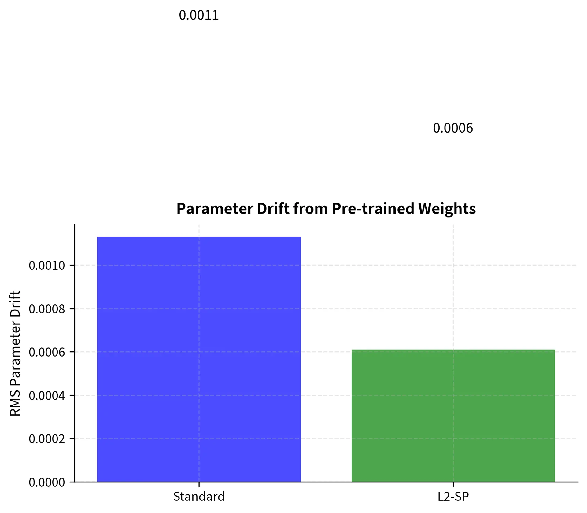
The L2-SP regularizer successfully constrains parameter drift while maintaining task performance. In practice, you would tune the regularization strength based on validation performance on both the target task and held-out tasks measuring prior capabilities.
Preserving Pre-trained Capabilities
Beyond mitigating forgetting during training, you need strategies to actively preserve the valuable capabilities that pre-trained models bring.
Layer-wise Learning Rates
Different layers encode different levels of abstraction. Earlier layers learn general features (syntax, basic semantics) while later layers specialize for the pre-training task. This suggests using different learning rates:
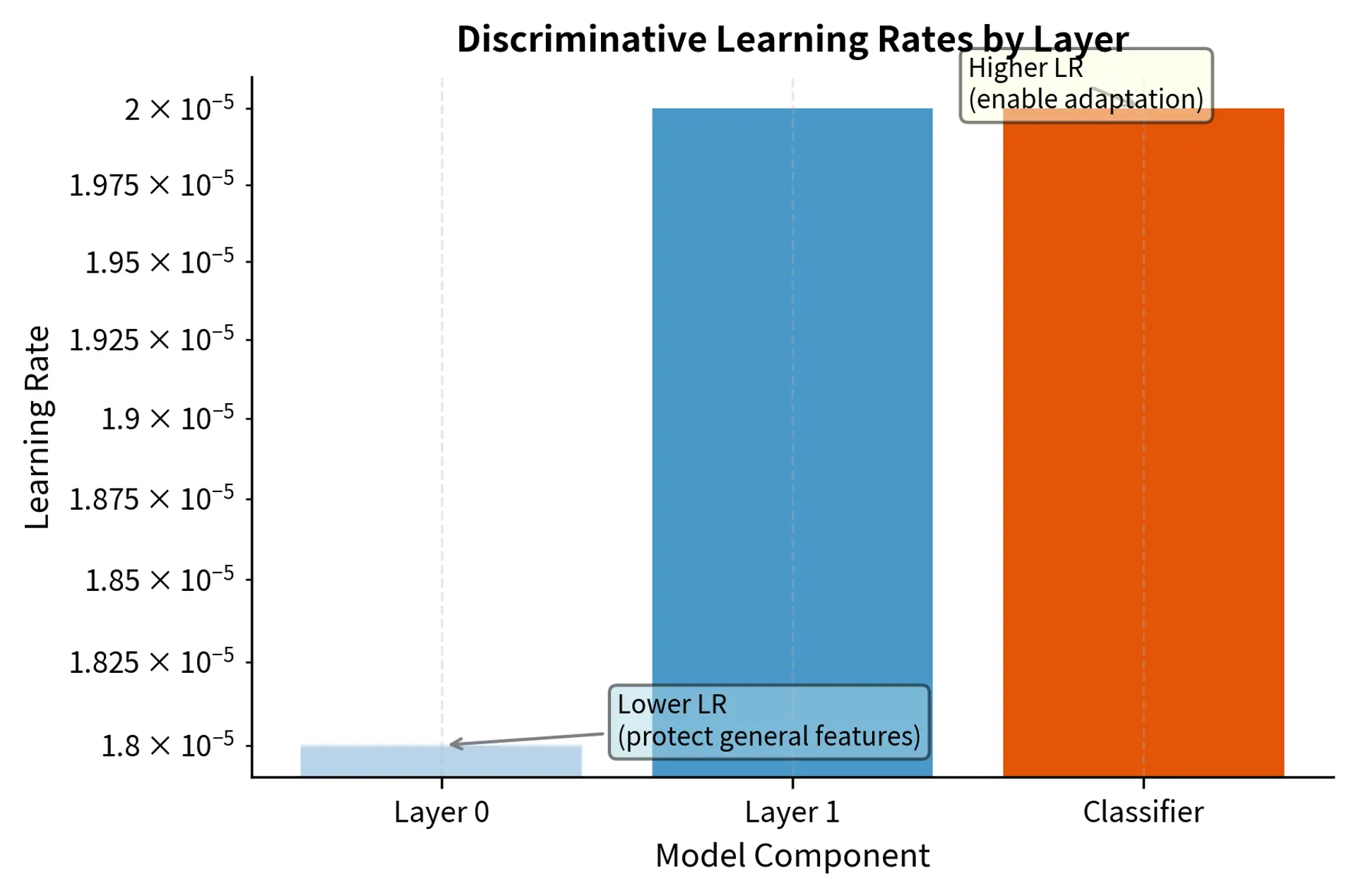
This discriminative schedule applies aggressive updates to the task-specific classifier head while protecting the foundational features in early encoder layers with much smaller learning rates.
Gradual Unfreezing
Another approach is to initially freeze early layers and progressively unfreeze them during training:
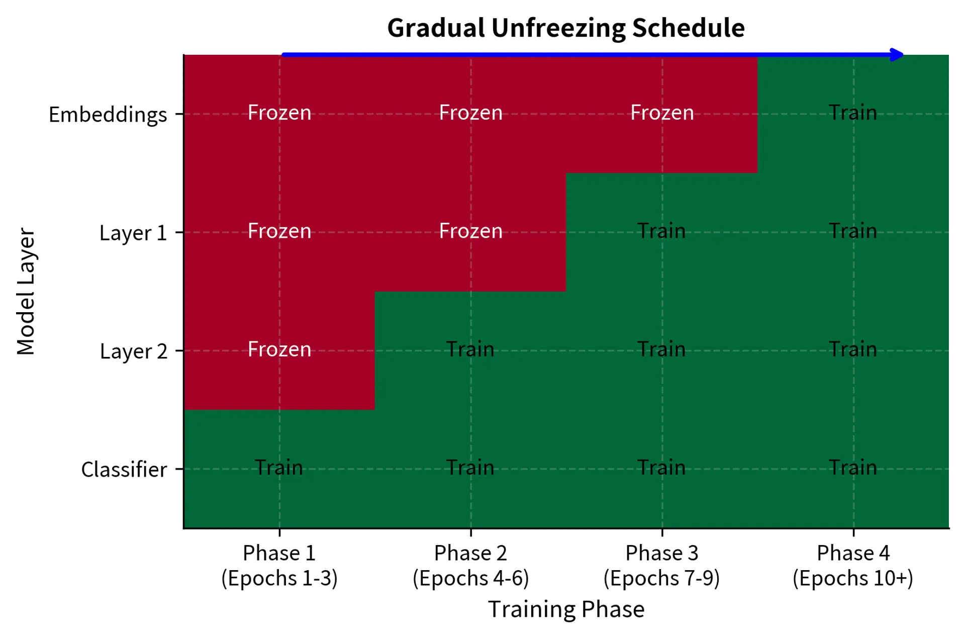
Starting with most parameters frozen limits the plasticity of the model, preventing large weight updates that could destroy pre-trained knowledge. As training stabilizes, more layers are unfrozen to allow fine-grained adaptation.
Evaluation-Driven Stopping
Perhaps the most reliable way to preserve capabilities is to continuously monitor them:
The trainer detects that the performance drop (from 0.85 to 0.75) exceeds the allowable threshold, triggering a stop signal. This active monitoring acts as a safety brake, ensuring that the model retains essential capabilities throughout the fine-tuning process.
Limitations and Impact
Catastrophic forgetting remains an active research area with no perfect solutions. Each mitigation strategy involves trade-offs.
Regularization approaches like EWC and L2-SP slow forgetting but cannot eliminate it entirely. They also require storing additional information (Fisher matrices or original weights) and add hyperparameters that need tuning. For very long fine-tuning runs or significantly different task distributions, regularization alone may be insufficient.
Replay methods effectively maintain prior performance but require access to pre-training data, which may not be available for proprietary models. They also increase training time and memory requirements proportionally to how much replay data is included. Generative replay avoids the data storage problem but introduces its own errors through imperfect generation.
Architecture-based solutions like adapter layers offer the strongest forgetting prevention by freezing original weights entirely, but they constrain the model's ability to adapt representations. For tasks requiring significant representational change, frozen architectures may underperform full fine-tuning. We'll explore these approaches in detail in the upcoming PEFT chapters, where methods like LoRA provide a compelling middle ground.
The broader impact of understanding catastrophic forgetting extends beyond single-model fine-tuning. Continual learning systems that must adapt to streaming data face forgetting challenges at every update. Multi-task models must balance performance across many objectives simultaneously. Even alignment techniques like RLHF must carefully manage forgetting to prevent models from losing capabilities while learning to follow instructions.
Summary
Catastrophic forgetting occurs when fine-tuning overwrites the neural representations responsible for pre-trained capabilities. This phenomenon stems from the fundamental stability-plasticity dilemma: neural networks must be plastic enough to learn new tasks but stable enough to retain old knowledge.
Measuring forgetting requires evaluating models on held-out tasks representing prior capabilities, using metrics like backward transfer, perplexity degradation, or benchmark suite performance. Without measurement, forgetting goes undetected until deployment reveals unexpected failures.
Mitigation strategies span multiple approaches. Regularization methods like L2-SP and EWC penalize parameter drift from pre-trained values. Replay methods mix prior task data into fine-tuning batches. Architecture methods freeze original weights while adding trainable components. Learning rate strategies apply differential updates across layers.
Preserving pre-trained capabilities requires combining these techniques with careful monitoring. Layer-wise learning rates protect general features in early layers. Gradual unfreezing allows controlled adaptation. Most importantly, continuous evaluation on capability benchmarks enables early detection and intervention when forgetting exceeds acceptable thresholds.
As we'll see in the Fine-tuning Learning Rates chapter, the choice of learning rate schedule profoundly impacts both task learning and forgetting dynamics. The PEFT methods covered later offer particularly elegant solutions by adding small trainable modules while keeping pre-trained weights completely frozen, effectively eliminating forgetting at the cost of reduced adaptation flexibility.
Quiz
Ready to test your understanding? Take this quick quiz to reinforce what you've learned about catastrophic forgetting and strategies to mitigate it during fine-tuning.

Comments