Fine-tuning Learning Rates: LLRD, Warmup & Decay Strategies

Michael BrenndoerferNovember 27, 202542 min read

Master learning rate strategies for fine-tuning transformers. Learn discriminative fine-tuning, layer-wise decay, warmup schedules, and decay methods.

Reading Level

Choose your expertise level to adjust how many terms are explained. Beginners see more tooltips, experts see fewer to maintain reading flow. Hover over underlined terms for instant definitions.

Fine-tuning Learning Rates

When you fine-tune a pre-trained language model, choosing the right learning rate is more important than when training from scratch. A learning rate that works well for pre-training can destroy months of computational effort in minutes of fine-tuning. Conversely, a learning rate that's too small might never adapt the model to your task. The challenge lies in finding the narrow band of learning rates that enable meaningful adaptation without erasing the knowledge the model has already acquired. This chapter explores specialized learning rate strategies developed specifically for fine-tuning: discriminative fine-tuning, layer-wise learning rate decay, warmup schedules, and decay strategies that help navigate the delicate balance between adaptation and preservation.

The Fine-tuning Learning Rate Challenge

As we discussed in the previous chapter on catastrophic forgetting, fine-tuning involves a fundamental tension. You want the model to learn task-specific patterns, but you don't want to overwrite the rich linguistic knowledge acquired during pre-training. Learning rates sit at the heart of this tension because they directly control how much each gradient update changes the model's parameters.

During pre-training, models typically use learning rates between 10410^{-4} and 10310^{-3} with the Adam optimizer. These relatively large rates help the model explore the parameter space efficiently when learning from scratch. At this stage, there is nothing to preserve: the model begins with random weights, and large updates are not only safe but necessary for making rapid progress across billions of training tokens. But fine-tuning presents a fundamentally different scenario: you're starting from a carefully optimized point that already captures meaningful language structure. The pre-trained weights represent a local minimum that took enormous computational resources to reach, and this minimum encodes valuable knowledge about syntax, semantics, and world knowledge. Large updates can push parameters far from this optimum, destroying valuable representations that took the original training process millions of gradient steps to construct.

The standard solution is to use much smaller learning rates for fine-tuning, typically in the range of 10510^{-5} to 5×1055 \times 10^{-5} for BERT-style models. This reduction of roughly one to two orders of magnitude reflects the different nature of the optimization problem: rather than exploring a vast parameter landscape, we are making careful adjustments around an already-good solution. But even this simple observation raises deeper questions:

  • Should all layers receive the same learning rate?
  • Should the rate start small and grow, or start larger and decay?
  • How do these choices interact with different model architectures?

The strategies we'll explore in this chapter emerged from attempts to answer these questions systematically. Rather than treating fine-tuning as simply "training with a smaller learning rate," we have developed nuanced approaches that consider which parts of the model need to change and by how much.

Discriminative Fine-tuning

Discriminative fine-tuning assigns different learning rates to different parts of the model based on the intuition that not all parameters should adapt equally. This approach recognizes that a pre-trained language model is not a monolithic entity but rather a hierarchy of representations, each capturing different levels of linguistic abstraction.

Discriminative Fine-tuning

A fine-tuning strategy where different parameter groups receive different learning rates, typically with lower layers learning more slowly than higher layers to preserve general features while allowing task-specific adaptation.

Different layers in a neural network learn different features. Deep networks develop a natural hierarchy: lower layers in transformer models capture general linguistic patterns such as tokenization boundaries, basic syntax, and fundamental semantic relationships. These patterns apply broadly across virtually any language task you might encounter. Higher layers capture more task-specific features that build on these foundations, developing representations increasingly tailored to the pre-training objective. When fine-tuning for a specific task, you want to:

  1. Preserve lower-layer representations: These capture transferable knowledge that applies across tasks. The basic understanding of language structure, word relationships, and syntactic patterns learned in these layers will be useful regardless of whether you're doing sentiment analysis, question answering, or named entity recognition.
  2. Adapt higher-layer representations: These need to specialize for your specific task. The upper layers, which were optimized for masked language modeling or next-token prediction, need to reconfigure their representations to support your new objective.
  3. Train the new task head aggressively: This is entirely task-specific and needs full adaptation. Unlike the pre-trained backbone, the task head starts from random initialization and has no prior knowledge to preserve.

This suggests a natural structure: assign progressively larger learning rates as you move up through the network. Lower layers receive small learning rates that allow only gentle adjustments, nudging the representations slightly while preserving their overall structure. Higher layers receive larger rates that enable substantial adaptation to the new task. The task-specific head receives the largest rate of all, allowing it to rapidly learn the mapping from pre-trained representations to task outputs.

Mathematical Formulation

To implement discriminative fine-tuning, we need a principled way to assign learning rates across layers. The most common approach uses geometric decay, where each step down the network reduces the learning rate by a constant factor. This creates a smooth gradient of adaptation rates that respects the hierarchical nature of the model's representations.

Let's denote the base learning rate as η\eta and define a decay factor ξ\xi (typically between 0.9 and 0.95). For a model with LL layers, layer ll receives learning rate:

ηl=ηξLl\eta_l = \eta \cdot \xi^{L-l}

where:

  • ηl\eta_l: the learning rate assigned to layer ll (the value we compute)
  • η\eta: the base learning rate assigned to the top layer (typically the highest rate in the backbone)
  • ξ\xi: the multiplicative decay factor (usually 0.9 to 0.95), which scales down the rate for each step down the network
  • LL: the total number of layers in the model
  • ll: the index of the current layer (where l=Ll=L is the top layer, l=1l=1 is the bottom transformer layer, and embeddings are treated as l=0l=0)

The key to this formulation is the exponent LlL-l, which represents the layer's distance from the top of the network. Consider how this distance-based calculation works in practice. The top layer (l=Ll = L) has a distance of 0, so ξ0=1\xi^0=1, receiving the full base rate η\eta. Each subsequent layer down increases the distance by 1, compounding the decay factor ξ\xi. This compounding effect means that the learning rate doesn't just decrease linearly as we move down the network; instead, it decreases geometrically, with each layer receiving a fixed fraction of the rate assigned to the layer above it.

Geometric decay ensures that the relative difference between adjacent layers remains constant throughout the network. If layer 10 receives 95% of the rate of layer 11, then layer 5 also receives 95% of the rate of layer 6. This proportional relationship ensures that the adaptation dynamics remain consistent regardless of which part of the network we examine.

For a 12-layer BERT model with η=2×10⁵\eta = 2 \times 10^{-5} and ξ=0.95\xi = 0.95:

Learning rates for each layer of a 12-layer BERT model using Layer-wise Learning Rate Decay (LLRD) with a decay factor of 0.95. The rates decrease geometrically from the top layer to the embeddings, ensuring that lower layers remain more stable while upper layers adapt more to the specific task.
LayerLearning Rate
Layer 12 (top)2.0×1052.0 \times 10^{-5}
Layer 111.9×1051.9 \times 10^{-5}
Layer 101.81×1051.81 \times 10^{-5}
Layer 61.47×1051.47 \times 10^{-5}
Layer 1 (bottom)1.14×1051.14 \times 10^{-5}
Embeddings1.08×1051.08 \times 10^{-5}

This creates a smooth gradient of adaptation rates throughout the network. Notice that even the bottom layer still receives a meaningful learning rate, roughly half of the top layer's rate. This reflects the philosophy that all layers should be allowed to adapt, just to different degrees. The embeddings receive the lowest rate because they encode fundamental vocabulary semantics that should remain maximally stable across different downstream tasks.

Out[2]:
Visualization
Using Python 3.11.13 environment at: /Users/michaelbrenndoerfer/tinker/mb/.venv
Audited 2 packages in 13ms
Geometric decay of learning rates across transformer layers. The exponential relationship means lower layers receive progressively smaller updates, preserving general linguistic knowledge while allowing upper layers to adapt to task-specific patterns.

Layer-wise Learning Rate Decay

Layer-wise learning rate decay (LLRD) is the most common implementation of discriminative fine-tuning for transformer models. It was popularized by the ULMFiT paper and has become standard practice for fine-tuning BERT and similar models. While the underlying mathematics are identical to discriminative fine-tuning, LLRD specifically emphasizes the layer-by-layer structure of modern transformer architectures and has been refined through extensive empirical study.

Why Layer Position Matters

LLRD works because transformer representations are hierarchical. Varying learning rates by layer is based on research into what each layer learns during pre-training. Research on probing tasks, where simple classifiers are trained on frozen layer representations, has systematically mapped out this hierarchy:

  • Embedding layers capture lexical semantics and basic word relationships. At this level, the model encodes what words mean in isolation and how they relate to other words with similar meanings. These representations are highly general and transfer well to virtually any downstream task.
  • Lower transformer layers (1-4 in BERT) capture syntactic structure and local dependencies. These layers develop sensitivity to part-of-speech patterns, phrase boundaries, and local word order. They learn to distinguish nouns from verbs, identify subject-verb relationships, and recognize basic grammatical patterns.
  • Middle layers (5-8) develop richer semantic representations that integrate local syntactic information with broader contextual meaning. These layers begin to capture coreference, semantic roles, and the flow of meaning across sentences.
  • Upper layers (9-12) capture task-relevant features that are more specific to the pre-training objective. For a model trained with masked language modeling, these layers specialize in predicting missing words given context. This specialization is valuable but also means these representations are most tightly coupled to the pre-training task.

When fine-tuning for a downstream task, the upper layers typically need the most adaptation because they were optimized for the pre-training task (like masked language modeling) rather than your specific objective. Lower layers, which capture more universal linguistic properties that any NLP task would benefit from, need less adjustment. Aggressive updates to lower layers risk disrupting the carefully learned syntactic and semantic foundations that the entire model relies upon.

Implementing LLRD for Transformers

For transformer models, we typically define parameter groups corresponding to:

  1. Embedding layer: Token embeddings and position embeddings
  2. Encoder/decoder layers: Each transformer block as a separate group
  3. Task head: The newly added classification or regression layer
In[3]:
Code
!uv pip install transformers torch
import torch
import torch.nn as nn
import math
from transformers import AutoModel, BertConfig, BertModel
import matplotlib.pyplot as plt
import numpy as np

def create_llrd_parameter_groups(model, base_lr=2e-5, decay_factor=0.95, weight_decay=0.01):
    """
    Create parameter groups with layer-wise learning rate decay.
    
    Args:
        model: HuggingFace transformer model
        base_lr: Learning rate for the top layer
        decay_factor: Multiplicative decay per layer
        weight_decay: L2 regularization strength
    
    Returns:
        List of parameter group dictionaries for optimizer
    """
    parameter_groups = []
    
    # Get all encoder layers
    encoder_layers = model.encoder.layer if hasattr(model, 'encoder') else model.transformer.h
    num_layers = len(encoder_layers)
    
    # Embedding parameters - lowest learning rate
    embedding_params = []
    for name, param in model.named_parameters():
        if ('embedding' in name.lower() or 'embed' in name.lower()) and param.requires_grad:
            embedding_params.append(param)
    
    if embedding_params:
        embedding_lr = base_lr * (decay_factor ** num_layers)
        parameter_groups.append({
            'params': embedding_params,
            'lr': embedding_lr,
            'weight_decay': weight_decay,
            'group_name': 'embeddings'
        })
    
    # Layer-wise parameters
    for layer_idx, layer in enumerate(encoder_layers):
        layer_lr = base_lr * (decay_factor ** (num_layers - 1 - layer_idx))
        layer_params = [p for p in layer.parameters() if p.requires_grad]
        
        if layer_params:
            parameter_groups.append({
                'params': layer_params,
                'lr': layer_lr,
                'weight_decay': weight_decay,
                'group_name': f'layer_{layer_idx}'
            })
    
    # Pooler and any remaining top-level parameters
    remaining_params = []
    assigned_params = set()
    for group in parameter_groups:
        for p in group['params']:
            assigned_params.add(id(p))
    
    for name, param in model.named_parameters():
        if id(param) not in assigned_params and param.requires_grad:
            remaining_params.append(param)
    
    if remaining_params:
        parameter_groups.append({
            'params': remaining_params,
            'lr': base_lr,
            'weight_decay': weight_decay,
            'group_name': 'top'
        })
    
    return parameter_groups

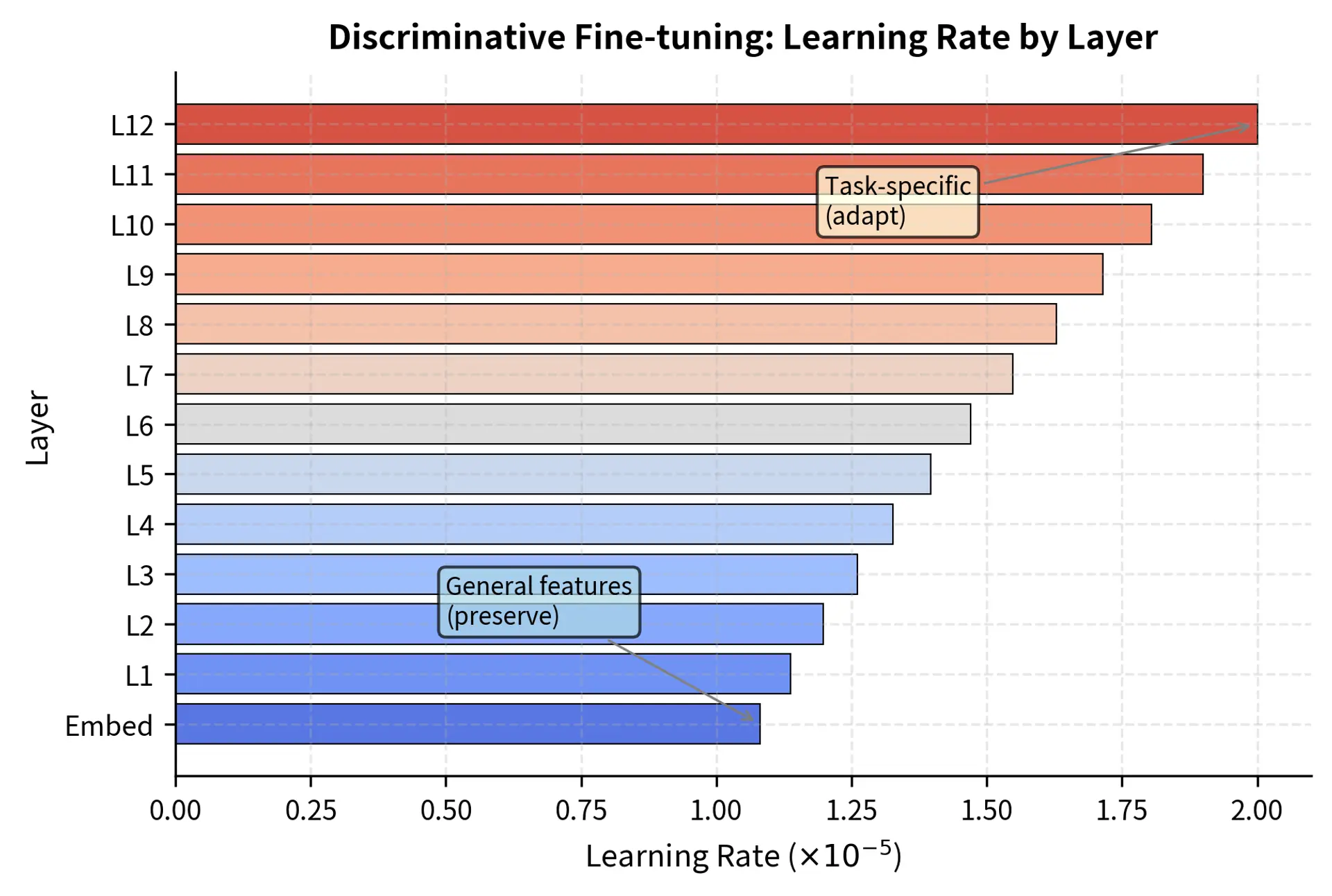
Let's examine the learning rate distribution across layers:

In[4]:
Code
# Create a sample configuration to visualize
base_lr = 2e-5
decay_factor = 0.95
num_layers = 12

lr_distribution = {}
lr_distribution["embeddings"] = base_lr * (decay_factor**num_layers)

for layer_idx in range(num_layers):
    lr = base_lr * (decay_factor ** (num_layers - 1 - layer_idx))
    lr_distribution[f"layer_{layer_idx}"] = lr

lr_distribution["task_head"] = base_lr / decay_factor

# Prepare lists for visualization
layer_names = list(lr_distribution.keys())
learning_rates = list(lr_distribution.values())
Out[5]:
Console
Learning rate distribution with LLRD:
Layer           Learning Rate  
------------------------------
embeddings      1.08e-05
layer_0         1.14e-05
layer_1         1.20e-05
layer_2         1.26e-05
layer_3         1.33e-05
layer_4         1.40e-05
layer_5         1.47e-05
layer_6         1.55e-05
layer_7         1.63e-05
layer_8         1.71e-05
layer_9         1.81e-05
layer_10        1.90e-05
layer_11        2.00e-05
task_head       2.11e-05

Learning rates decay geometrically through the layers. The embeddings receive the lowest rate (1.08×1051.08 \times 10^{-5}), ensuring the model's fundamental vocabulary representations remain stable. This stability is crucial because the embedding layer defines the basic semantic space that all other layers build upon. If embeddings shift dramatically during fine-tuning, the higher layers must relearn how to interpret these shifted representations, potentially causing cascading disruptions throughout the network.

In[6]:
Code
import matplotlib.pyplot as plt
import numpy as np

plt.rcParams.update(
    {
        "figure.figsize": (6.0, 4.0),
        "figure.dpi": 300,
        "figure.constrained_layout.use": True,
        "font.family": "sans-serif",
        "font.sans-serif": [
            "Noto Sans CJK SC",
            "Apple SD Gothic Neo",
            "DejaVu Sans",
            "Arial",
        ],
        "font.size": 10,
        "axes.titlesize": 11,
        "axes.titleweight": "bold",
        "axes.titlepad": 8,
        "axes.labelsize": 10,
        "axes.labelpad": 4,
        "xtick.labelsize": 9,
        "ytick.labelsize": 9,
        "legend.fontsize": 9,
        "legend.title_fontsize": 10,
        "legend.frameon": True,
        "legend.loc": "best",
        "lines.linewidth": 1.5,
        "lines.markersize": 5,
        "axes.grid": True,
        "grid.alpha": 0.3,
        "grid.linestyle": "--",
        "axes.spines.top": False,
        "axes.spines.right": False,
        "axes.prop_cycle": plt.cycler(
            color=["#1f77b4", "#ff7f0e", "#2ca02c", "#d62728", "#7f7f7f"]
        ),
    }
)

fig, ax = plt.subplots()

x_positions = np.arange(len(layer_names))
colors = plt.cm.viridis(np.linspace(0.2, 0.8, len(layer_names)))

bars = ax.bar(x_positions, [lr * 1e5 for lr in learning_rates], color=colors)
ax.set_xticks(x_positions)
ax.set_xticklabels(layer_names, rotation=45, ha="right")
ax.set_ylabel(r"Learning Rate ($\times 10^{-5}$)")
ax.set_xlabel("Model Component")
ax.set_title(
    f"Layer-wise Learning Rate Decay (LLRD)\nBase LR = {base_lr:.0e}, Decay = {decay_factor}"
)

# Add value labels on bars
for bar, lr in zip(bars, learning_rates):
    ax.text(
        bar.get_x() + bar.get_width() / 2,
        bar.get_height() + 0.02,
        f"{lr:.1e}",
        ha="center",
        va="bottom",
        fontsize=8,
        rotation=45,
    )

This visualization shows the learning rate hierarchy. The embeddings and lower layers remain relatively stable to preserve fundamental language understanding, while the learning rate increases exponentially toward the task head to facilitate rapid adaptation to the new problem. The smooth progression ensures that no single layer boundary experiences a dramatic discontinuity in adaptation rates, which could create optimization instabilities.

Choosing the Decay Factor
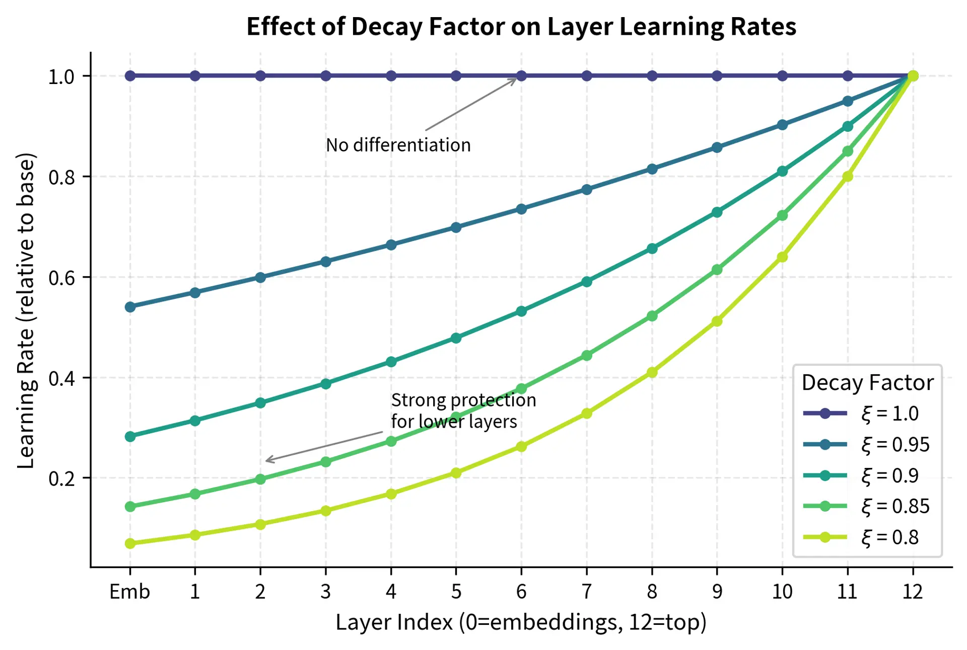
The decay factor ξ\xi controls how aggressively learning rates differ between layers, and choosing the right value requires balancing two competing concerns. A decay factor too close to 1.0 provides insufficient differentiation between layers, losing the benefits of discriminative fine-tuning. A decay factor too small may prevent lower layers from adapting at all, which can be problematic if your task requires the model to learn new low-level patterns. The optimal value depends on your task and how much the pre-trained representations need to change:

  • ξ=1.0\xi = 1.0: No decay; all layers receive the same learning rate (standard fine-tuning). This is equivalent to ignoring the hierarchical structure of the network and may be appropriate when you have abundant data and the task differs substantially from pre-training.
  • ξ=0.95\xi = 0.95: Gentle decay; good default for most NLP tasks. This creates roughly a 2:1 ratio between the top and bottom layer learning rates, providing differentiation while still allowing all layers to adapt meaningfully.
  • ξ=0.9\xi = 0.9: Moderate decay; useful when lower layers should change minimally. This creates approximately a 3:1 ratio and is appropriate when you have limited data or when the pre-training domain closely matches your target task.
  • ξ=0.8\xi = 0.8: Aggressive decay; for tasks very similar to pre-training. This can create ratios of 5:1 or greater and essentially "freezes" the lower layers by giving them very small learning rates.

Empirically, values between 0.9 and 0.95 work well for most transformer fine-tuning scenarios. When in doubt, 0.95 provides a safe starting point that rarely hurts performance and often helps.

Out[8]:
Visualization
Impact of decay factor on learning rate distribution across layers. Higher decay factors (closer to 1.0) create more uniform learning rates, while lower factors create steeper gradients that protect lower layers more aggressively.

Learning Rate Warmup for Fine-tuning

Warmup refers to starting training with a very small learning rate and gradually increasing it to the target value. This technique is especially important for fine-tuning. While warmup was originally motivated by considerations specific to the Adam optimizer and very deep networks, its benefits during fine-tuning arise from slightly different concerns.

Why Warmup Matters for Fine-tuning

At the start of fine-tuning, several factors make large learning rates dangerous. Understanding these factors helps explain why warmup, which might seem like an unnecessary complication, provides substantial practical benefits:

  1. Task head initialization: The newly added classification head is randomly initialized while the pre-trained backbone is well-optimized. This creates an asymmetry in the network: the backbone produces meaningful representations, but the randomly initialized head transforms these into essentially random predictions. The gradients flowing back from this random head can be large and poorly directed. Large initial updates from the random head can destabilize the entire network, propagating noise deep into the pre-trained layers. Warmup allows the task head to "catch up" to the backbone before the learning rate becomes large enough to cause damage.

  2. Gradient variance: Early mini-batches may not be representative of the full dataset, leading to noisy gradient estimates. The first few batches might happen to contain unusual examples or reflect sampling artifacts rather than the true data distribution. Small learning rates during warmup prevent over-reacting to this noise, giving the optimizer time to aggregate gradient information from more representative samples.

  3. Adam statistics: As we discussed in the Adam optimizer chapter, Adam maintains running estimates of gradient moments, specifically the first moment (mean) and second moment (variance) of the gradients. These estimates are unreliable early in training because they are initialized to zero and require many updates to become accurate. The bias correction terms in Adam help, but they don't fully compensate for the lack of historical information. Warmup gives these moment estimates time to stabilize before making large parameter updates that rely on their accuracy.

Linear warmup

The most common warmup schedule increases the learning rate linearly from 0 to the target value. This approach is simple to implement, easy to understand, and effective in practice:

ηt=tTwarmupηtarget\eta_t = \frac{t}{T_{\text{warmup}}} \cdot \eta_{\text{target}}

where:

  • ηt\eta_t: the learning rate at step tt
  • tt: the current training step
  • TwarmupT_{\text{warmup}}: the total number of warmup steps (defining the duration of the ramp-up phase)
  • ηtarget\eta_{\text{target}}: the target learning rate to reach at the end of warmup (the peak rate)

The ratio tTwarmup\frac{t}{T_{\text{warmup}}} represents the fraction of the warmup phase completed, scaling the learning rate linearly from 0 up to ηtarget\eta_{\text{target}}. At step 0, this ratio equals 0, so the learning rate is 0. At step TwarmupT_{\text{warmup}}, the ratio equals 1, so the learning rate reaches its target. The linear relationship means that the learning rate increases by a constant amount at each step, providing a predictable and smooth ramp-up.

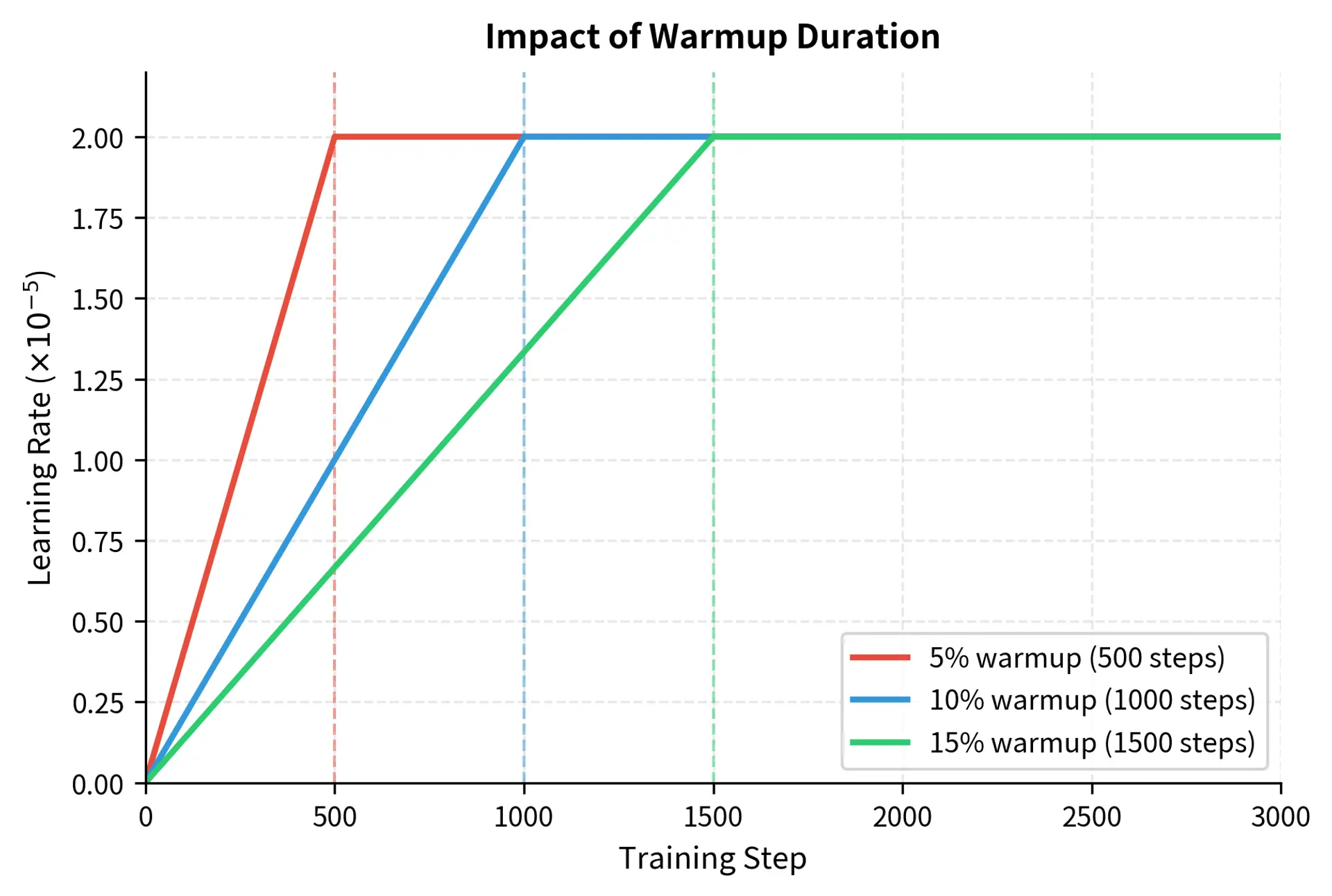
For fine-tuning, warmup typically spans 5-10% of total training steps. For a fine-tuning run of 10,000 steps, you might use 500-1,000 warmup steps. This duration allows Adam's moment estimates to stabilize and the task head to begin learning patterns without wasting training time.

In[9]:
Code
def linear_warmup_schedule(step, warmup_steps, target_lr):
    """
    Calculate learning rate during linear warmup.

    Args:
        step: Current training step
        warmup_steps: Number of warmup steps
        target_lr: Target learning rate after warmup

    Returns:
        Learning rate for this step
    """
    if step < warmup_steps:
        return target_lr * (step / warmup_steps)
    return target_lr


def warmup_with_decay_schedule(step, warmup_steps, total_steps, target_lr):
    """
    Linear warmup followed by linear decay to zero.

    This is the most common schedule for fine-tuning BERT-style models.
    """
    if step < warmup_steps:
        # Linear warmup
        return target_lr * (step / warmup_steps)
    else:
        # Linear decay
        decay_steps = total_steps - warmup_steps
        remaining_steps = total_steps - step
        return target_lr * (remaining_steps / decay_steps)

Let's visualize the warmup schedule:

In[10]:
Code
import numpy as np
import matplotlib.pyplot as plt

plt.rcParams.update(
    {
        "figure.figsize": (6.0, 4.0),
        "figure.dpi": 300,
        "figure.constrained_layout.use": True,
        "font.family": "sans-serif",
        "font.sans-serif": [
            "Noto Sans CJK SC",
            "Apple SD Gothic Neo",
            "DejaVu Sans",
            "Arial",
        ],
        "font.size": 10,
        "axes.titlesize": 11,
        "axes.titleweight": "bold",
        "axes.titlepad": 8,
        "axes.labelsize": 10,
        "axes.labelpad": 4,
        "xtick.labelsize": 9,
        "ytick.labelsize": 9,
        "legend.fontsize": 9,
        "legend.title_fontsize": 10,
        "legend.frameon": True,
        "legend.loc": "best",
        "lines.linewidth": 1.5,
        "lines.markersize": 5,
        "axes.grid": True,
        "grid.alpha": 0.3,
        "grid.linestyle": "--",
        "axes.spines.top": False,
        "axes.spines.right": False,
        "axes.prop_cycle": plt.cycler(
            color=["#1f77b4", "#ff7f0e", "#2ca02c", "#d62728", "#7f7f7f"]
        ),
    }
)

total_steps = 10000
warmup_steps = 1000
target_lr = 2e-5

steps = np.arange(total_steps)
lrs = [linear_warmup_schedule(s, warmup_steps, target_lr) for s in steps]

fig, ax = plt.subplots()
ax.plot(steps, [lr * 1e5 for lr in lrs], linewidth=2)
ax.axvline(x=warmup_steps, color="red", linestyle="--", label="End of warmup")
ax.fill_between(
    steps[: warmup_steps + 1],
    0,
    [lr * 1e5 for lr in lrs[: warmup_steps + 1]],
    alpha=0.3,
    color="orange",
    label="Warmup phase",
)
ax.set_xlabel("Training Step")
ax.set_ylabel(r"Learning Rate ($\times 10^{-5}$)")
ax.set_title("Linear Warmup Schedule")
ax.legend()
ax.set_xlim(0, total_steps)
ax.set_ylim(0, target_lr * 1.1 * 1e5)

This schedule prevents the optimizer from making dangerously large updates during the initial training phase, when gradient estimates are most volatile. The shaded warmup region represents the protective phase where the model's pre-trained knowledge is most vulnerable to disruption.

Out[12]:
Visualization
Comparison of different warmup durations. Shorter warmup (5%) reaches peak learning rate quickly but may destabilize training. Longer warmup (15%) provides more stability but delays the main training phase.

Gradual Unfreezing as Warmup

A more aggressive warmup strategy combines warmup with gradual unfreezing. Instead of training all layers from the start, you begin by training only the task head, then progressively unfreeze layers from top to bottom:

  1. Epoch 1: Train only the task head
  2. Epoch 2: Unfreeze top transformer layers
  3. Epoch 3: Unfreeze middle layers
  4. Epoch 4+: Train all layers

This approach, introduced in ULMFiT, provides an extreme form of "warmup" where lower layers literally receive zero gradient until later in training. The philosophy is that by the time lower layers are unfrozen, the task head and upper layers have already adapted substantially, providing more stable and informative gradients. While effective, gradual unfreezing requires more epochs and careful tuning of the unfreezing schedule. It has fallen somewhat out of favor for transformer fine-tuning because LLRD achieves similar goals with less complexity, but it remains a useful technique when maximum caution is warranted.

Learning Rate Decay

After warmup completes, learning rate decay schedules reduce the rate throughout training. This helps the model converge to a stable minimum rather than oscillating around it. The intuition is that large learning rates are useful early in training when the model needs to make significant adjustments, but become counterproductive later when the model is close to a good solution and only needs fine adjustments.

Linear Decay

The simplest decay schedule reduces the learning rate linearly to zero (or some minimum value) by the end of training. This approach provides a steady, predictable reduction in learning rate that is easy to reason about and implement:

ηt=ηtarget(1tTwarmupTtotalTwarmup)\eta_t = \eta_{\text{target}} \cdot \left(1 - \frac{t - T_{\text{warmup}}}{T_{\text{total}} - T_{\text{warmup}}}\right)

where:

  • ηt\eta_t: the learning rate at step tt
  • ηtarget\eta_{\text{target}}: the learning rate at the start of decay (end of warmup)
  • tt: the current training step
  • TwarmupT_{\text{warmup}}: the step number where decay begins
  • TtotalT_{\text{total}}: the total number of training steps

The structure of this formula becomes clearer when we break it into parts. The fraction tTwarmupTtotalTwarmup\frac{t - T_{\text{warmup}}}{T_{\text{total}} - T_{\text{warmup}}} represents the progress through the decay phase, ranging from 0 at the start of decay to 1 at the final step. Subtracting this from 1 yields the remaining proportion of the learning rate, creating a steady linear decline from ηtarget\eta_{\text{target}} down to 0. At each step during the decay phase, the learning rate decreases by exactly the same amount, ensuring a uniform reduction throughout training.

This is the default schedule for most BERT fine-tuning recipes because it strikes a reasonable balance between simplicity and effectiveness.

Cosine Decay

Cosine decay provides a smoother transition that decays slowly at first, accelerates in the middle, and slows again near the end. This schedule has become increasingly popular because it maintains higher learning rates for longer during the middle of training, allowing the optimizer more opportunity to explore the loss landscape before settling into a final minimum:

ηt=ηmin+ηtargetηmin2(1+cos(πtTwarmupTtotalTwarmup))\eta_t = \eta_{\text{min}} + \frac{\eta_{\text{target}} - \eta_{\text{min}}}{2} \cdot \left(1 + \cos\left(\pi \cdot \frac{t - T_{\text{warmup}}}{T_{\text{total}} - T_{\text{warmup}}}\right)\right)

where:

  • ηt\eta_t: the learning rate at step tt
  • ηmin\eta_{\text{min}}: the minimum learning rate to reach at the end of training
  • ηtarget\eta_{\text{target}}: the target learning rate at the start of decay
  • tt: the current training step
  • TwarmupT_{\text{warmup}}: the step number where decay begins
  • TtotalT_{\text{total}}: the total number of training steps

We can trace the mathematical transformations to see how this formula produces an S-curve:

  1. Progress Ratio: The term tTwarmupTtotalTwarmup\frac{t - T_{\text{warmup}}}{T_{\text{total}} - T_{\text{warmup}}} goes from 0 to 1 as training proceeds through the decay phase. This is the same progress measure used in linear decay.
  2. Angle Mapping: Multiplying by π\pi converts this linear progress to an angle from 0 to π\pi radians. This mapping is what transforms linear progress into the characteristic cosine shape.
  3. Cosine Transform: Taking the cosine of this angle produces values that vary smoothly. At the start of decay, cos(0)=1\cos(0) = 1, and at the end, cos(π)=1\cos(\pi) = -1. Crucially, the rate of change of cosine is zero at both endpoints and maximal in the middle.
  4. Scaling: The term 1+cos()1 + \cos(\dots) shifts the range from [1,1][-1, 1] to [0,2][0, 2]. This is then halved (yielding a range of [0,1][0, 1]) and scaled by the learning rate difference (ηtargetηmin)(\eta_{\text{target}} - \eta_{\text{min}}). Adding ηmin\eta_{\text{min}} shifts the final result to the desired range.

This results in a learning rate that decreases slowly at the start and end of training, with a faster decrease in the middle.

In[13]:
Code
import math


def cosine_decay_schedule(step, warmup_steps, total_steps, target_lr, min_lr=0):
    """
    Linear warmup followed by cosine decay.

    Args:
        step: Current training step
        warmup_steps: Number of warmup steps
        total_steps: Total number of training steps
        target_lr: Target learning rate after warmup
        min_lr: Minimum learning rate at end of training
    """
    if step < warmup_steps:
        return target_lr * (step / warmup_steps)
    else:
        progress = (step - warmup_steps) / (total_steps - warmup_steps)
        return min_lr + (target_lr - min_lr) * 0.5 * (
            1 + math.cos(math.pi * progress)
        )


def polynomial_decay_schedule(
    step, warmup_steps, total_steps, target_lr, min_lr=0, power=1.0
):
    """
    Linear warmup followed by polynomial decay.

    Power=1.0 gives linear decay, power=2.0 gives quadratic decay.
    """
    if step < warmup_steps:
        return target_lr * (step / warmup_steps)
    else:
        progress = (step - warmup_steps) / (total_steps - warmup_steps)
        decay = (1 - progress) ** power
        return min_lr + (target_lr - min_lr) * decay

Let's compare these decay schedules:

In[14]:
Code
import numpy as np
import matplotlib.pyplot as plt

plt.rcParams.update(
    {
        "figure.figsize": (6.0, 4.0),
        "figure.dpi": 300,
        "figure.constrained_layout.use": True,
        "font.family": "sans-serif",
        "font.sans-serif": [
            "Noto Sans CJK SC",
            "Apple SD Gothic Neo",
            "DejaVu Sans",
            "Arial",
        ],
        "font.size": 10,
        "axes.titlesize": 11,
        "axes.titleweight": "bold",
        "axes.titlepad": 8,
        "axes.labelsize": 10,
        "axes.labelpad": 4,
        "xtick.labelsize": 9,
        "ytick.labelsize": 9,
        "legend.fontsize": 9,
        "legend.title_fontsize": 10,
        "legend.frameon": True,
        "legend.loc": "best",
        "lines.linewidth": 1.5,
        "lines.markersize": 5,
        "axes.grid": True,
        "grid.alpha": 0.3,
        "grid.linestyle": "--",
        "axes.spines.top": False,
        "axes.spines.right": False,
        "axes.prop_cycle": plt.cycler(
            color=["#1f77b4", "#ff7f0e", "#2ca02c", "#d62728", "#7f7f7f"]
        ),
    }
)

total_steps = 10000
warmup_steps = 1000
target_lr = 2e-5

steps = np.arange(total_steps)

linear_lrs = [
    warmup_with_decay_schedule(s, warmup_steps, total_steps, target_lr)
    for s in steps
]
cosine_lrs = [
    cosine_decay_schedule(s, warmup_steps, total_steps, target_lr)
    for s in steps
]
poly2_lrs = [
    polynomial_decay_schedule(
        s, warmup_steps, total_steps, target_lr, power=2.0
    )
    for s in steps
]

fig, ax = plt.subplots()
ax.plot(
    steps, [lr * 1e5 for lr in linear_lrs], label="Linear decay", linewidth=2
)
ax.plot(
    steps, [lr * 1e5 for lr in cosine_lrs], label="Cosine decay", linewidth=2
)
ax.plot(
    steps, [lr * 1e5 for lr in poly2_lrs], label="Polynomial (p=2)", linewidth=2
)
ax.axvline(
    x=warmup_steps, color="gray", linestyle="--", alpha=0.5, label="End warmup"
)
ax.set_xlabel("Training Step")
ax.set_ylabel(r"Learning Rate ($\times 10^{-5}$)")
ax.set_title("Comparison of Learning Rate Decay Schedules")
ax.legend()
ax.set_xlim(0, total_steps)

While all three schedules eventually reach zero, they allocate learning rate differently throughout training. Cosine decay maintains higher learning rates for longer in the middle of training, potentially allowing the model to escape local minima more effectively than linear decay. Polynomial decay with power 2 drops quickly at first and then more slowly, front-loading the high learning rate period. The choice between these schedules represents a trade-off between exploration and convergence speed.

Choosing a Decay Schedule

The choice of decay schedule depends on your training dynamics and the specific characteristics of your task:

  • Linear decay: Simple and effective; good default for short fine-tuning runs. The predictable reduction makes it easy to reason about training dynamics and diagnose issues.
  • Cosine decay: Often slightly better performance; allows more learning early and late in training. The gentler decay at both ends can help the model both explore better initially and converge more precisely at the end.
  • Polynomial decay: Useful when you want to front-load learning (higher powers) or extend it (lower powers). This provides more control over the shape of the decay curve.

Empirically, cosine and linear decay perform similarly for most fine-tuning tasks, with cosine sometimes providing a small improvement. The difference is often smaller than the effect of other hyperparameters like the base learning rate or batch size, so either choice is reasonable for most applications.

Complete Implementation

Let's combine all these techniques into a complete fine-tuning setup. We'll create a training configuration that uses layer-wise learning rate decay, warmup, and cosine decay. This implementation demonstrates how the individual components we've discussed work together in practice.

In[16]:
Code
from torch.optim import AdamW
from torch.optim.lr_scheduler import LambdaLR

import math


class FineTuningConfig:
    """Configuration for fine-tuning with advanced learning rate strategies."""

    def __init__(
        self,
        base_lr=2e-5,
        llrd_decay=0.95,
        weight_decay=0.01,
        warmup_ratio=0.1,
        num_training_steps=10000,
        schedule="cosine",
    ):
        self.base_lr = base_lr
        self.llrd_decay = llrd_decay
        self.weight_decay = weight_decay
        self.warmup_ratio = warmup_ratio
        self.num_training_steps = num_training_steps
        self.warmup_steps = int(warmup_ratio * num_training_steps)
        self.schedule = schedule


def create_optimizer_and_scheduler(model, task_head, config):
    """
    Create optimizer with LLRD and scheduler with warmup + decay.

    Args:
        model: Pre-trained transformer model
        task_head: Task-specific classification head
        config: FineTuningConfig instance

    Returns:
        Tuple of (optimizer, scheduler)
    """
    # Get encoder layers for LLRD
    if hasattr(model, "encoder"):
        encoder_layers = list(model.encoder.layer)
    elif hasattr(model, "transformer"):
        encoder_layers = list(model.transformer.h)
    else:
        encoder_layers = []

    num_layers = len(encoder_layers)
    parameter_groups = []

    # Embeddings - lowest learning rate
    embedding_params = []
    for name, param in model.named_parameters():
        if "embed" in name.lower() and param.requires_grad:
            embedding_params.append(param)

    if embedding_params:
        embedding_lr = config.base_lr * (config.llrd_decay**num_layers)
        parameter_groups.append(
            {
                "params": embedding_params,
                "lr": embedding_lr,
                "weight_decay": config.weight_decay,
            }
        )

    # Encoder layers with LLRD
    processed_params = set(id(p) for p in embedding_params)

    for layer_idx, layer in enumerate(encoder_layers):
        layer_lr = config.base_lr * (
            config.llrd_decay ** (num_layers - 1 - layer_idx)
        )
        layer_params = [
            p
            for p in layer.parameters()
            if p.requires_grad and id(p) not in processed_params
        ]

        if layer_params:
            parameter_groups.append(
                {
                    "params": layer_params,
                    "lr": layer_lr,
                    "weight_decay": config.weight_decay,
                }
            )
            processed_params.update(id(p) for p in layer_params)

    # Remaining model parameters (pooler, etc.)
    remaining_params = [
        p
        for name, p in model.named_parameters()
        if p.requires_grad and id(p) not in processed_params
    ]

    if remaining_params:
        parameter_groups.append(
            {
                "params": remaining_params,
                "lr": config.base_lr,
                "weight_decay": config.weight_decay,
            }
        )

    # Task head - highest learning rate (often 10x base)
    task_head_lr = config.base_lr * 10
    parameter_groups.append(
        {
            "params": list(task_head.parameters()),
            "lr": task_head_lr,
            "weight_decay": config.weight_decay,
        }
    )

    # Create optimizer
    optimizer = AdamW(parameter_groups, betas=(0.9, 0.999), eps=1e-8)

    # Create scheduler
    def lr_lambda(current_step):
        if current_step < config.warmup_steps:
            return float(current_step) / float(max(1, config.warmup_steps))

        if config.schedule == "linear":
            progress = float(current_step - config.warmup_steps) / float(
                max(1, config.num_training_steps - config.warmup_steps)
            )
            return max(0.0, 1.0 - progress)

        elif config.schedule == "cosine":
            progress = float(current_step - config.warmup_steps) / float(
                max(1, config.num_training_steps - config.warmup_steps)
            )
            return max(0.0, 0.5 * (1.0 + math.cos(math.pi * progress)))

        return 1.0

    scheduler = LambdaLR(optimizer, lr_lambda)

    return optimizer, scheduler

Let's see this in action with a simple classification task:

In[17]:
Code
import torch
from transformers import BertConfig, BertModel

# Create a tiny model for demonstration (avoids downloading weights)
bert_config = BertConfig(
    hidden_size=128,
    num_hidden_layers=2,
    num_attention_heads=2,
    intermediate_size=512,
)
model = BertModel(bert_config)


# Create a simple task head
class ClassificationHead(torch.nn.Module):
    def __init__(self, hidden_size, num_classes):
        super().__init__()
        self.dropout = torch.nn.Dropout(0.1)
        self.classifier = torch.nn.Linear(hidden_size, num_classes)

    def forward(self, pooled_output):
        x = self.dropout(pooled_output)
        return self.classifier(x)


task_head = ClassificationHead(model.config.hidden_size, num_classes=2)

# Create fine-tuning configuration
config = FineTuningConfig(
    base_lr=2e-5,
    llrd_decay=0.95,
    warmup_ratio=0.1,
    num_training_steps=1000,
    schedule="cosine",
)

# Create optimizer and scheduler
optimizer, scheduler = create_optimizer_and_scheduler(model, task_head, config)

# Calculate parameter stats for display
param_group_stats = []
for i, group in enumerate(optimizer.param_groups):
    num_params = sum(p.numel() for p in group["params"])
    param_group_stats.append(
        {"group_idx": i, "lr": group["lr"], "num_params": num_params}
    )
Out[18]:
Console
Fine-tuning Configuration
==================================================
Base learning rate: 2.00e-05
LLRD decay factor: 0.95
Warmup steps: 100
Total training steps: 1,000
Schedule: cosine

Learning Rates per Parameter Group:
--------------------------------------------------
Group 0: LR = 0.00e+00, Params = 3,972,864
Group 1: LR = 0.00e+00, Params = 198,272
Group 2: LR = 0.00e+00, Params = 198,272
Group 3: LR = 0.00e+00, Params = 16,512
Group 4: LR = 0.00e+00, Params = 258

In this configuration, the task head has a higher learning rate (2.00×1042.00 \times 10^{-4}) than the embeddings. This hierarchy ensures that the randomly initialized task head can adapt quickly while the pre-trained backbone layers are updated more cautiously.

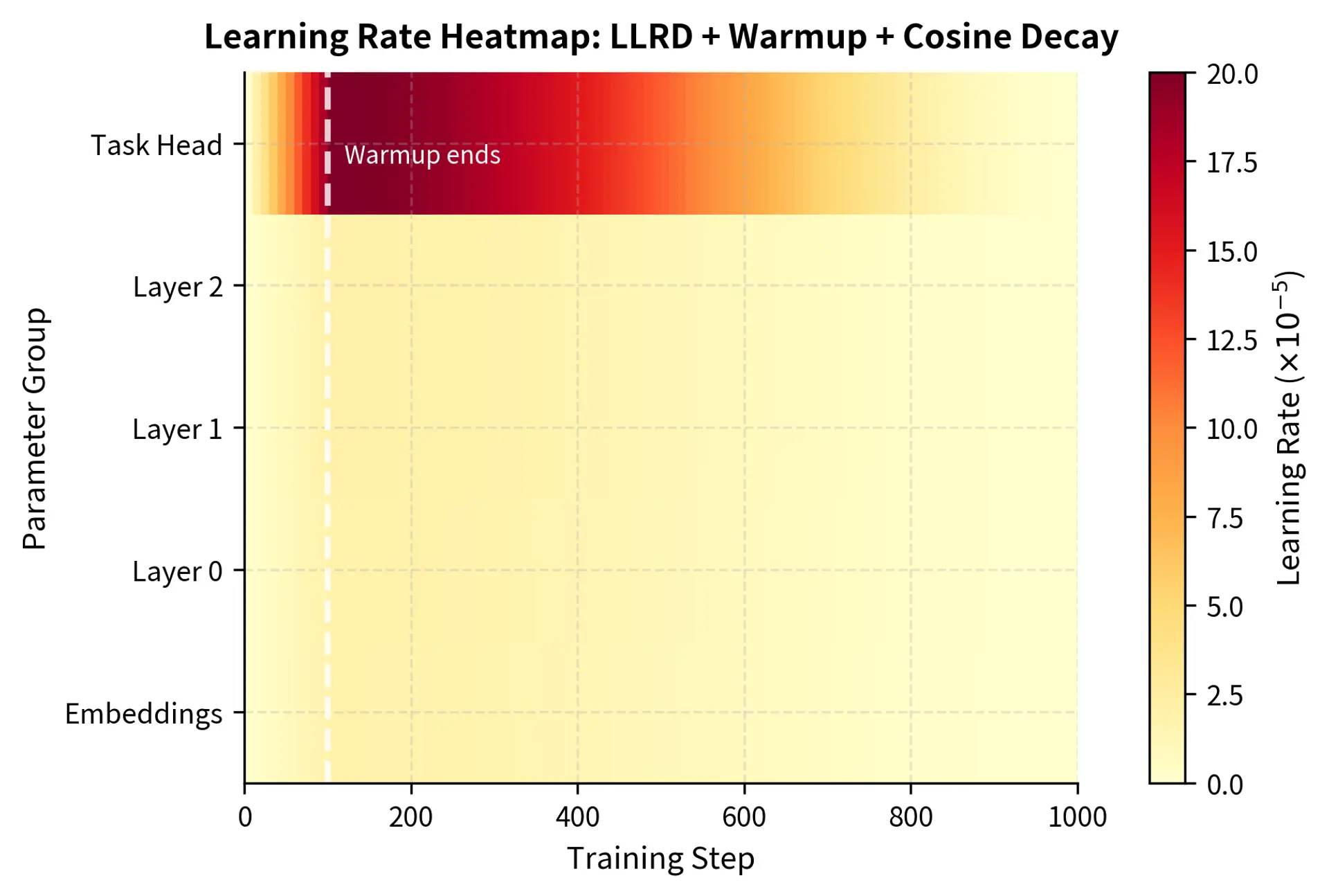
Now let's simulate a training run and visualize how learning rates evolve:

In[19]:
Code
import matplotlib.pyplot as plt
import numpy as np

plt.rcParams.update(
    {
        "figure.figsize": (6.0, 4.0),
        "figure.dpi": 300,
        "figure.constrained_layout.use": True,
        "font.family": "sans-serif",
        "font.sans-serif": [
            "Noto Sans CJK SC",
            "Apple SD Gothic Neo",
            "DejaVu Sans",
            "Arial",
        ],
        "font.size": 10,
        "axes.titlesize": 11,
        "axes.titleweight": "bold",
        "axes.titlepad": 8,
        "axes.labelsize": 10,
        "axes.labelpad": 4,
        "xtick.labelsize": 9,
        "ytick.labelsize": 9,
        "legend.fontsize": 9,
        "legend.title_fontsize": 10,
        "legend.frameon": True,
        "legend.loc": "best",
        "lines.linewidth": 1.5,
        "lines.markersize": 5,
        "axes.grid": True,
        "grid.alpha": 0.3,
        "grid.linestyle": "--",
        "axes.spines.top": False,
        "axes.spines.right": False,
        "axes.prop_cycle": plt.cycler(
            color=["#1f77b4", "#ff7f0e", "#2ca02c", "#d62728", "#7f7f7f"]
        ),
    }
)

# Reset optimizer state and track learning rates over training
optimizer, scheduler = create_optimizer_and_scheduler(model, task_head, config)

# Track LRs for selected groups
lr_history = {f"Group {i}": [] for i in range(len(optimizer.param_groups))}

for step in range(config.num_training_steps):
    # Record current learning rates
    for i, group in enumerate(optimizer.param_groups):
        lr_history[f"Group {i}"].append(group["lr"])

    # Step the scheduler (in real training, this happens after optimizer.step())
    scheduler.step()

# Plot selected groups for clarity
fig, ax = plt.subplots()
steps = np.arange(config.num_training_steps)

# Plot embedding layer (lowest LR)
ax.plot(
    steps,
    [lr * 1e5 for lr in lr_history["Group 0"]],
    label="Embeddings",
    linewidth=2,
    alpha=0.8,
)

# Plot a middle transformer layer
mid_group = len(optimizer.param_groups) // 2
ax.plot(
    steps,
    [lr * 1e5 for lr in lr_history[f"Group {mid_group}"]],
    label="Middle layers",
    linewidth=2,
    alpha=0.8,
)

# Plot top transformer layer
ax.plot(
    steps,
    [lr * 1e5 for lr in lr_history[f"Group {len(optimizer.param_groups) - 2}"]],
    label="Top layers",
    linewidth=2,
    alpha=0.8,
)

# Plot task head (highest LR)
ax.plot(
    steps,
    [lr * 1e5 for lr in lr_history[f"Group {len(optimizer.param_groups) - 1}"]],
    label="Task head",
    linewidth=2,
    alpha=0.8,
)

ax.axvline(x=config.warmup_steps, color="gray", linestyle="--", alpha=0.5)
ax.annotate(
    "End warmup",
    xy=(config.warmup_steps, 0),
    xytext=(config.warmup_steps + 50, config.base_lr * 1e5),
    fontsize=10,
    alpha=0.7,
)

ax.set_xlabel("Training Step")
ax.set_ylabel(r"Learning Rate ($\times 10^{-5}$)")
ax.set_title(
    "Learning Rate Evolution During Fine-tuning\n(LLRD + Warmup + Cosine Decay)"
)
ax.legend(loc="upper right")
ax.set_xlim(0, config.num_training_steps)

The separate trajectories show the combined effect of our strategies: all layers warm up together, but they peak at different values due to LLRD, and then decay in sync according to the cosine schedule. The task head's learning rate (shown at the top) is an order of magnitude larger than the embeddings' rate throughout training, reflecting our confidence that the task head needs rapid adaptation while the embeddings should remain relatively stable.

Out[21]:
Visualization
Heatmap showing learning rate evolution across all layers during fine-tuning. The color intensity represents learning rate magnitude, clearly showing the combined effect of LLRD (vertical gradient) and warmup plus decay (horizontal pattern).

Complete Training Loop Example

Here's how these components integrate into a complete fine-tuning loop:

In[37]:
Code
def fine_tune_model(
    model, task_head, train_dataloader, val_dataloader, config, device="cuda"
):
    """
    Complete fine-tuning loop with LLRD, warmup, and decay.
    """
    model.to(device)
    task_head.to(device)

    optimizer, scheduler = create_optimizer_and_scheduler(
        model, task_head, config
    )
    criterion = torch.nn.CrossEntropyLoss()

    model.train()
    task_head.train()

    global_step = 0
    best_val_accuracy = 0

    for epoch in range(num_epochs):
        epoch_loss = 0

        for batch in train_dataloader:
            input_ids = batch["input_ids"].to(device)
            attention_mask = batch["attention_mask"].to(device)
            labels = batch["labels"].to(device)

            # Forward pass
            outputs = model(input_ids, attention_mask=attention_mask)
            pooled_output = outputs.last_hidden_state[:, 0]  # CLS token
            logits = task_head(pooled_output)

            loss = criterion(logits, labels)

            # Backward pass
            optimizer.zero_grad()
            loss.backward()

            # Gradient clipping (important for stability)
            torch.nn.utils.clip_grad_norm_(
                list(model.parameters()) + list(task_head.parameters()),
                max_norm=1.0,
            )

            optimizer.step()
            scheduler.step()

            global_step += 1
            epoch_loss += loss.item()

            # Log learning rates periodically
            if global_step % 100 == 0:
                current_lr = scheduler.get_last_lr()[0]
                print(
                    f"Step {global_step}: Loss = {loss.item():.4f}, LR = {current_lr:.2e}"
                )

        # Validation
        val_accuracy = evaluate(model, task_head, val_dataloader, device)
        print(f"Epoch {epoch + 1}: Val Accuracy = {val_accuracy:.4f}")

        if val_accuracy > best_val_accuracy:
            best_val_accuracy = val_accuracy
            # Save best model checkpoint
            torch.save(
                {
                    "model_state_dict": model.state_dict(),
                    "task_head_state_dict": task_head.state_dict(),
                    "optimizer_state_dict": optimizer.state_dict(),
                },
                "best_model.pt",
            )

    return best_val_accuracy

Practical Guidelines

Based on extensive empirical research, here are practical recommendations for fine-tuning learning rates:

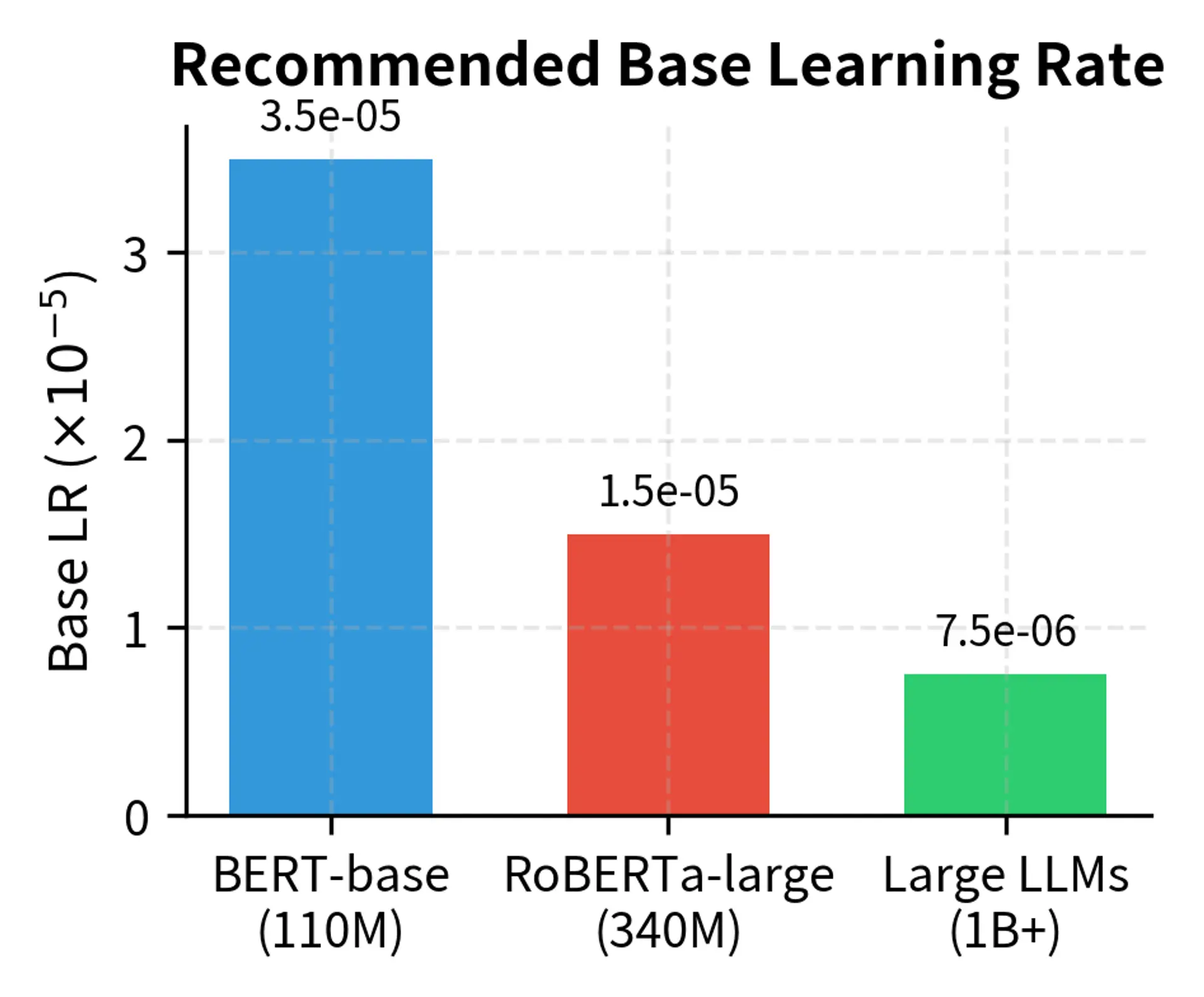
For BERT-base and similar models (110M parameters):

  • Base learning rate: 2×1052 \times 10^{-5} to 5×1055 \times 10^{-5}
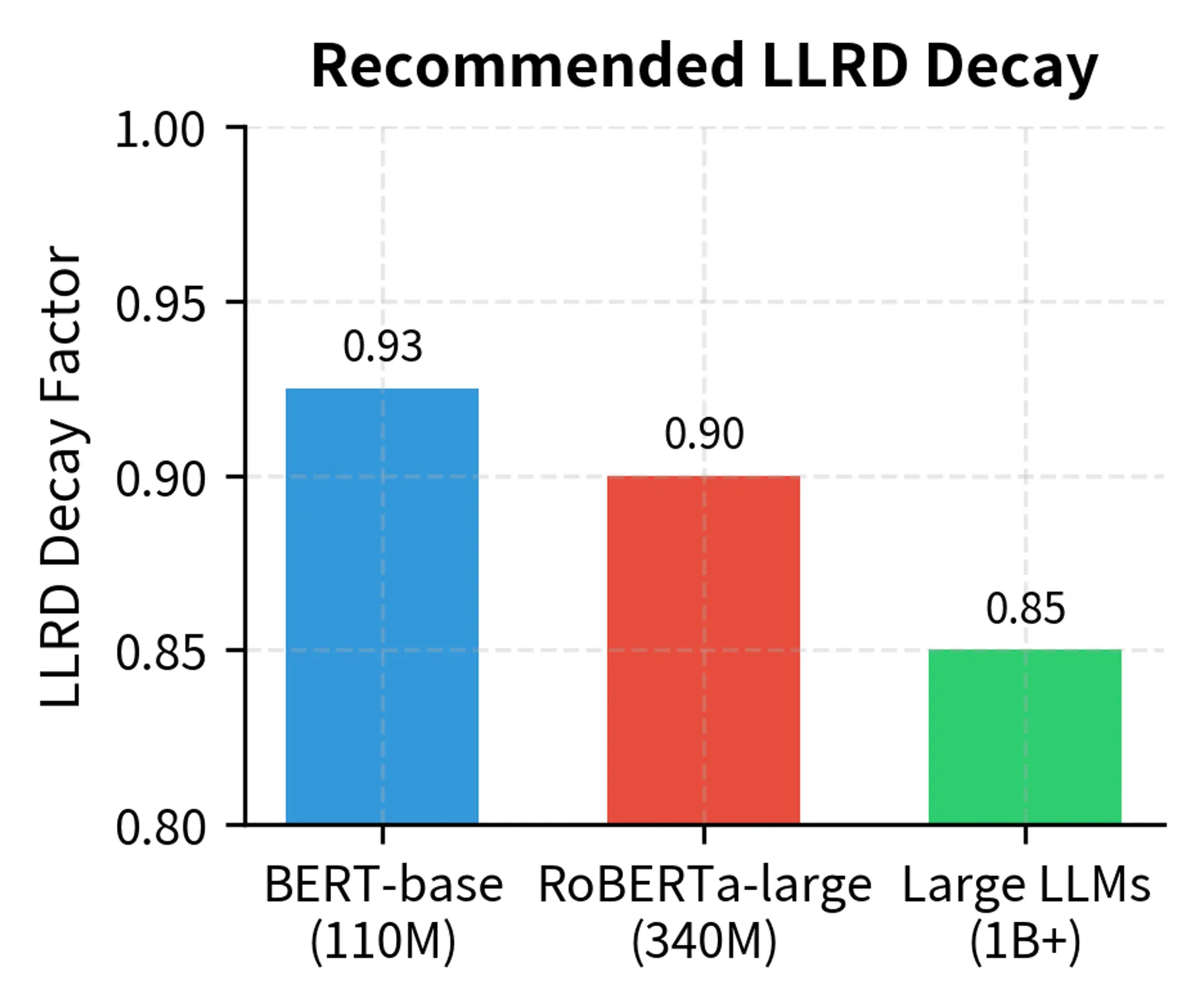
  • LLRD decay: 0.9 to 0.95
  • Warmup: 6-10% of training steps
  • Task head learning rate: 10× base rate

For larger models (GPT-2, RoBERTa-large, 340M+ parameters):

  • Base learning rate: 10510^{-5} to 2×1052 \times 10^{-5} (lower due to more layers)
  • LLRD decay: 0.85 to 0.95
  • Warmup: 10% of training steps
  • Consider lower weight decay (0.001 instead of 0.01)

For very large models (1B+ parameters):

  • Base learning rate: 5×1065 \times 10^{-6} to 10510^{-5}
  • More aggressive LLRD decay: 0.8 to 0.9
  • Longer warmup: 10-15% of training steps
  • Often better to use parameter-efficient methods like LoRA, which we'll cover in upcoming chapters

General principles:

  • Start with the lower end of learning rate ranges and increase if learning is too slow
  • Monitor both training loss and validation metrics; overfitting indicates the rate may be too high
  • If loss spikes early, increase warmup steps or decrease initial learning rate
  • If loss plateaus too early, try a higher learning rate or different decay schedule
Out[22]:
Visualization
Recommended base learning rates for different model sizes. Larger models like 1B+ parameter LLMs require significantly lower learning rates to maintain optimization stability.
Recommended layer-wise learning rate decay (LLRD) factors. Larger models benefit from more aggressive decay (lower factors) to more strongly preserve pre-trained lower-layer representations.

Limitations and Impact

These learning rate strategies have significantly improved fine-tuning results across many NLP tasks, but they come with important caveats.

The effectiveness of layer-wise learning rate decay depends on the assumption that lower layers capture more general features. While this holds for many tasks, it may not apply universally. For tasks that differ substantially from the pre-training distribution (such as fine-tuning an English model for code generation), the optimal learning rate hierarchy might differ from standard recommendations. Some practitioners have found that uniform learning rates perform just as well on certain tasks, suggesting that LLRD's benefits are task-dependent.

The interaction between these techniques and other regularization methods (dropout, weight decay, batch size) creates a complex optimization landscape. A learning rate that works perfectly with one dropout rate might be suboptimal with another. This interdependence means that comprehensive hyperparameter search often yields better results than following any single recipe, though this can be computationally expensive.

The computational overhead of implementing these strategies is minimal, but the engineering complexity is not. Maintaining separate learning rates for dozens of parameter groups, coordinating warmup schedules, and debugging learning rate issues all add development time. For rapid prototyping, uniform learning rates with basic warmup often provide 90% of the benefit with 10% of the complexity.

These techniques also don't address all fine-tuning challenges. Catastrophic forgetting can still occur even with optimal learning rates, particularly on small datasets or with many training epochs. As we'll explore in upcoming chapters on parameter-efficient fine-tuning, methods like LoRA offer complementary approaches that limit the number of parameters updated rather than just their learning rates.

Summary

Fine-tuning learning rates require careful consideration that goes beyond simply selecting a single value. The strategies covered in this chapter address different aspects of the fine-tuning challenge:

Layer-wise learning rate decay assigns different learning rates to different layers based on the principle that lower layers capture general features (requiring less adaptation) while upper layers capture task-specific features (requiring more adaptation). Using a decay factor between 0.9 and 0.95 across layers typically provides a good balance.

Learning rate warmup gradually increases the learning rate from zero during the first 5-10% of training. This stabilizes optimization by allowing Adam's moment estimates to accumulate and preventing the randomly initialized task head from destabilizing pre-trained weights.

Learning rate decay reduces the rate throughout training, helping the model converge to a stable minimum. Cosine and linear decay are both effective choices, with cosine sometimes providing slight improvements.

Combining these techniques creates a robust fine-tuning setup: warmup followed by decay, with different base rates for different layers. The task head typically receives 10× the base learning rate since it starts from random initialization and needs aggressive training.

These strategies represent one dimension of efficient fine-tuning. In the next chapter, we'll examine data efficiency: how to get the most out of limited labeled data when adapting pre-trained models to new tasks.

Quiz

Ready to test your understanding? Take this quick quiz to reinforce what you've learned about fine-tuning learning rate strategies.

Loading component...

Reference

BIBTEXAcademic
@misc{finetuninglearningratesllrdwarmupdecaystrategies, author = {Michael Brenndoerfer}, title = {Fine-tuning Learning Rates: LLRD, Warmup & Decay Strategies}, year = {2025}, url = {https://mbrenndoerfer.com/writing/fine-tuning-learning-rates-llrd-warmup-decay-transformers}, organization = {mbrenndoerfer.com}, note = {Accessed: 2025-01-01} }
APAAcademic
Michael Brenndoerfer (2025). Fine-tuning Learning Rates: LLRD, Warmup & Decay Strategies. Retrieved from https://mbrenndoerfer.com/writing/fine-tuning-learning-rates-llrd-warmup-decay-transformers
MLAAcademic
Michael Brenndoerfer. "Fine-tuning Learning Rates: LLRD, Warmup & Decay Strategies." 2026. Web. today. <https://mbrenndoerfer.com/writing/fine-tuning-learning-rates-llrd-warmup-decay-transformers>.
CHICAGOAcademic
Michael Brenndoerfer. "Fine-tuning Learning Rates: LLRD, Warmup & Decay Strategies." Accessed today. https://mbrenndoerfer.com/writing/fine-tuning-learning-rates-llrd-warmup-decay-transformers.
HARVARDAcademic
Michael Brenndoerfer (2025) 'Fine-tuning Learning Rates: LLRD, Warmup & Decay Strategies'. Available at: https://mbrenndoerfer.com/writing/fine-tuning-learning-rates-llrd-warmup-decay-transformers (Accessed: today).
SimpleBasic
Michael Brenndoerfer (2025). Fine-tuning Learning Rates: LLRD, Warmup & Decay Strategies. https://mbrenndoerfer.com/writing/fine-tuning-learning-rates-llrd-warmup-decay-transformers