Time Value of Money & Interest Rates: Finance Fundamentals

A dollar today is worth more than a dollar tomorrow. This simple observation underpins virtually every financial calculation you will encounter, from pricing bonds and valuing companies to structuring mortgages and retirement plans. The concept is called the time value of money (TVM), and understanding it is essential for anyone working in quantitative finance.

Why is money worth more today? Three reasons drive this phenomenon. First, money received today can be invested to earn a return, making it grow over time. Second, inflation erodes purchasing power, so a dollar today buys more than a dollar in the future. Third, there is uncertainty about whether promised future payments will actually materialize. These factors combine to create a fundamental asymmetry: present money is more valuable than future money.

The time value of money gives us a framework for comparing cash flows that occur at different points in time. Without this framework, how would you choose between receiving $1,000 today versus $1,100 in one year? Or evaluate a business that requires $1 million upfront but promises $200,000 annually for the next seven years? TVM provides the mathematical machinery to answer these questions rigorously.

Interest rates are the mechanism that links present and future values. They quantify the "price" of borrowing money or the "reward" for lending it. In quantitative finance, interest rates serve as the foundation for pricing nearly every financial instrument. Understanding how they work, how they compound, and how they are quoted across markets is critical knowledge that we will use throughout this book.

When you deposit money in an interest-bearing account, your balance grows over time. The process by which this growth occurs, and particularly how interest accumulates on previously earned interest, is called compounding. This concept drives both wealth accumulation and debt growth. Let's build up from the simplest case to the continuous limit used in derivatives pricing, understanding each step along the way.

Simple interest is the most basic form of interest calculation and serves as our conceptual starting point. Under simple interest, the interest accrues only on the original principal amount, never on accumulated interest. Think of it as a linear process: each period adds the same fixed amount of interest, regardless of how much has accumulated before. If you invest a principal $P$ at an annual interest rate $r$ for $t$ years, the future value is:

where:

• $FV$: future value of the investment
• $P$: principal amount (initial investment)
• $r$: annual interest rate (expressed as a decimal)
• $t$: time in years

The structure of this formula reveals its linear nature. The term $rt$ represents the total proportional increase: the rate $r$ multiplied by time $t$. When you add this to 1 (representing the original principal as 100%), you get the total growth factor. Multiplying by $P$ then scales this to your actual investment amount. Notice that time and rate enter symmetrically and additively. Doubling the time has exactly the same effect as doubling the rate.

For example, investing $1,000 at 5% simple interest for 3 years yields:

Notice that the interest earned ($150) equals the annual interest ($50) multiplied by the number of years (3). Simple interest grows linearly with time, which makes it straightforward to calculate but unrealistic for most financial applications. In the real world, lenders and investors expect to earn interest on their accumulated interest, a concept we turn to next.

In practice, interest typically compounds periodically. This means the interest earned in each period is added to the principal, and subsequent interest is calculated on this larger balance. The fundamental insight is that your money earns returns not just on your original investment, but on all the returns that investment has already generated. This creates exponential rather than linear growth, a distinction with profound implications over long time horizons.

To understand why compounding leads to exponential growth, consider what happens period by period. After the first compounding period, your balance is $P(1 + r/n)$. After the second period, interest is calculated on this new, larger balance, giving $P(1 + r/n)(1 + r/n) = P(1 + r/n)^2$. Each period multiplies the previous balance by the same growth factor, and multiplication repeated many times produces exponential behavior.

For an investment compounding $n$ times per year at annual rate $r$, the future value after $t$ years is:

where:

• $FV$: future value after $t$ years
• $P$: principal amount invested
• $r$: nominal annual interest rate (stated rate)
• $n$: number of compounding periods per year
• $t$: time in years
• $(1 + r/n)$: growth factor per compounding period
• $nt$: total number of compounding periods

The formula captures a key insight: each compounding period applies a small growth factor $(1 + r/n)$, and these compound multiplicatively over $nt$ total periods. The rate per period is $r/n$ because we divide the annual rate among $n$ periods, and the total number of periods is $nt$ because we have $n$ periods per year for $t$ years. More frequent compounding means smaller individual growth factors applied more times, which slightly increases total growth due to the "interest on interest" effect. This is because you begin earning interest on your interest sooner, so you don't have to wait as long for each interest payment to start generating its own returns.

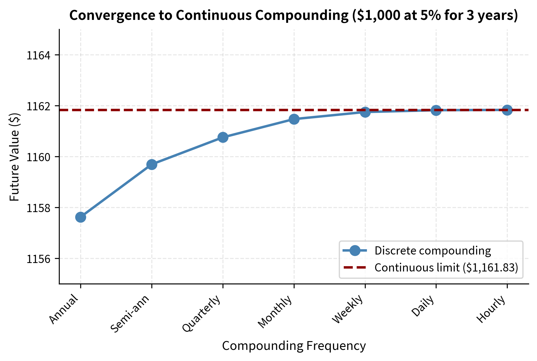
Let's compare different compounding frequencies for the same nominal rate:

As compounding frequency increases, the future value grows, but the incremental gains diminish. Moving from annual to semi-annual compounding adds about $3.80, while moving from monthly to daily adds only about $0.05. This pattern of diminishing returns suggests a natural limit as $n \to \infty$: no matter how frequently you compound, there is an upper bound on the growth you can achieve at a given rate. This limit is not merely a mathematical curiosity; it forms the basis for continuous compounding, the framework preferred in derivatives pricing.

Taking the limit as the compounding frequency approaches infinity gives us continuous compounding. Rather than compounding at discrete intervals like monthly, daily, or even every second, continuous compounding assumes that interest accrues and is reinvested at every instant. This is the standard framework used in derivatives pricing because it simplifies many calculations and produces elegant mathematical properties.

The continuous compounding formula emerges from taking the limit of the discrete formula as $n$ grows without bound:

where:

• $FV$: future value
• $P$: principal amount
• $r$: continuously compounded annual rate
• $t$: time in years
• $e$: Euler's number ($\approx 2.71828$)

This result relies on the fundamental limit $\lim_{n \to \infty}(1 + x/n)^n = e^x$, one of the most important limits in mathematics. To see why this limit makes sense intuitively, consider that as $n$ increases, each individual growth factor $(1 + r/n)$ gets closer to 1, but you apply more and more of them. These two effects, smaller factors applied more times, balance out to give a finite limit, and that limit happens to be the exponential function.

The exponential function $e^{rt}$ emerges naturally because continuous compounding represents the limiting case of infinitely many infinitesimally small growth events. This makes continuous compounding mathematically convenient: returns become additive in the logarithm, meaning $\ln(FV/P) = rt$. This logarithmic property greatly simplifies many calculations in derivatives pricing, because the return over multiple periods can be computed simply by adding up the returns over sub-periods, rather than multiplying growth factors together.

The difference between daily and continuous compounding is negligible for practical purposes. However, continuous compounding has elegant mathematical properties. Returns become additive (the log of a product equals the sum of logs), and many differential equations in finance have cleaner solutions.

Let's visualize how future value grows under different compounding schemes:

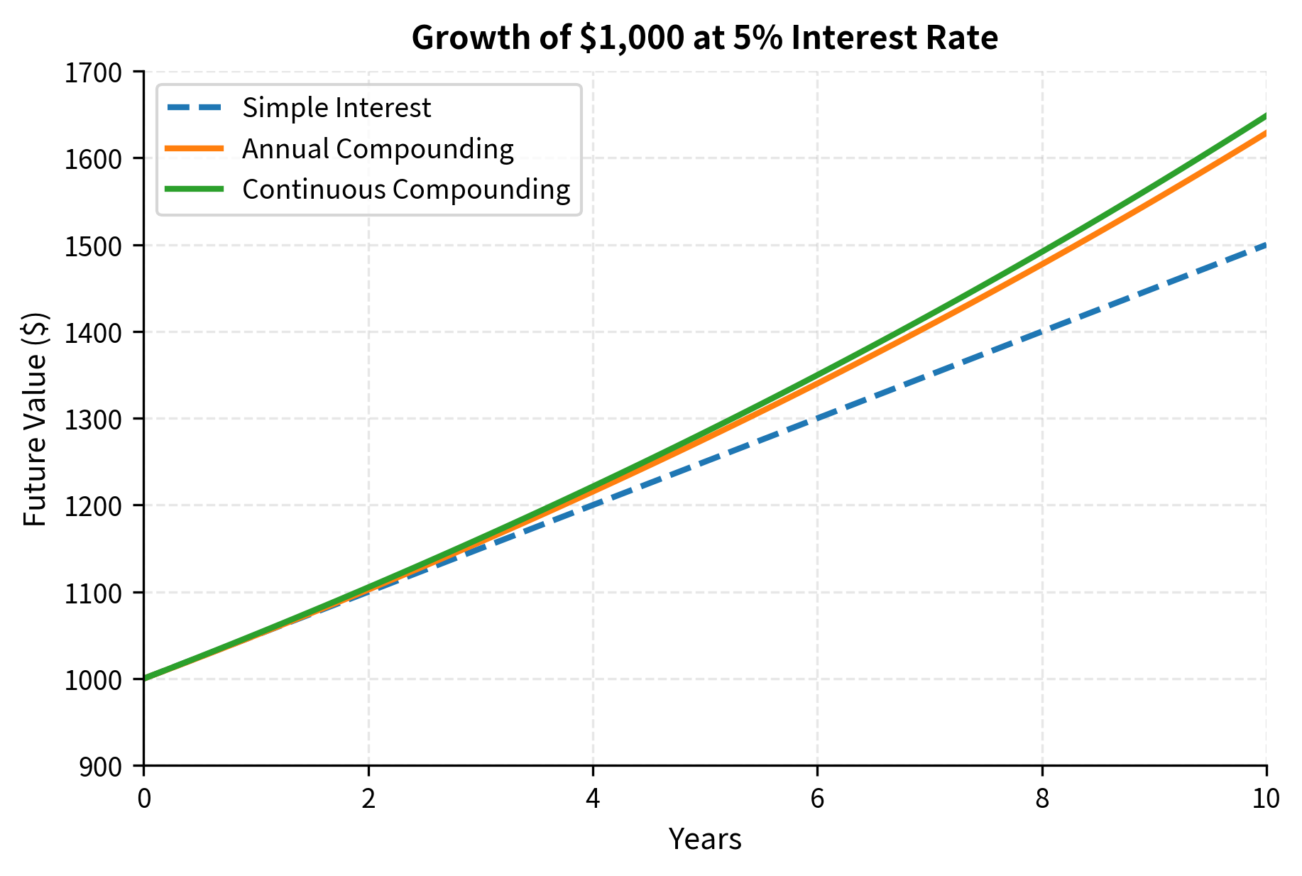
The chart reveals that simple interest grows linearly while compound interest grows exponentially. Over short horizons, the differences are small. Over long horizons, they become dramatic. This explains why compound interest accumulates so powerfully over time.

While future value answers "what will this be worth later?", present value addresses the inverse question: "what is a future payment worth today?" This is the more common question in finance, because we frequently need to value future cash flows. When you price a bond, evaluate an investment project, or determine how much to save for retirement, you are fundamentally asking present value questions.

Discounting is the reverse of compounding. If compounding moves money forward in time by multiplying by growth factors, discounting moves money backward in time by dividing by those same factors. Algebraically, we unwrap the future value formula to find the present value:

where:

• $PV$: present value (value today)
• $FV$: future value (amount to be received)
• $r$: discount rate (annual)
• $t$: time until payment (years)
• $(1 + r)^{-t}$: the discount factor

The discount factor $(1 + r)^{-t}$ answers a simple question: what fraction of a future dollar is worth today? For positive interest rates, this fraction is always less than one, reflecting the fundamental principle that a dollar today is worth more than a dollar tomorrow. The higher the discount rate or the longer the time horizon, the smaller the discount factor becomes. Distant or heavily discounted cash flows contribute little to present value.

For continuous compounding, the discounting formula takes an even more elegant form:

where:

• $PV$: present value
• $FV$: future value
• $r$: continuously compounded discount rate
• $t$: time in years
• $e^{-rt}$: the continuous discount factor, always between 0 and 1 for positive rates

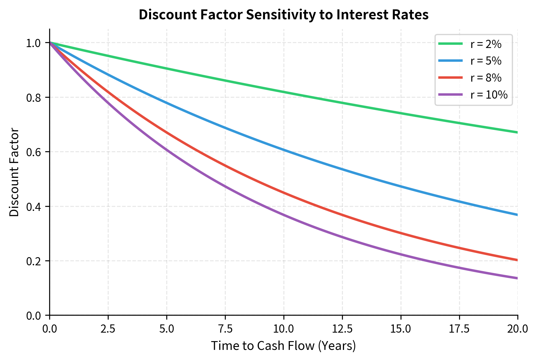
The negative exponent in $e^{-rt}$ reflects that we are reversing the compounding process. Just as $e^{rt}$ grows money forward in time by a factor that increases with time, $e^{-rt}$ shrinks it backward by a factor that decreases with time. The symmetry works as follows: if continuous compounding with rate $r$ takes $1 today to $e^{rt}$ at time $t$, then discounting takes $e^{rt}$ at time $t$ back to $1 today. The discount factor decays exponentially with time, meaning distant cash flows are worth progressively less today. The decay is steeper for higher discount rates.

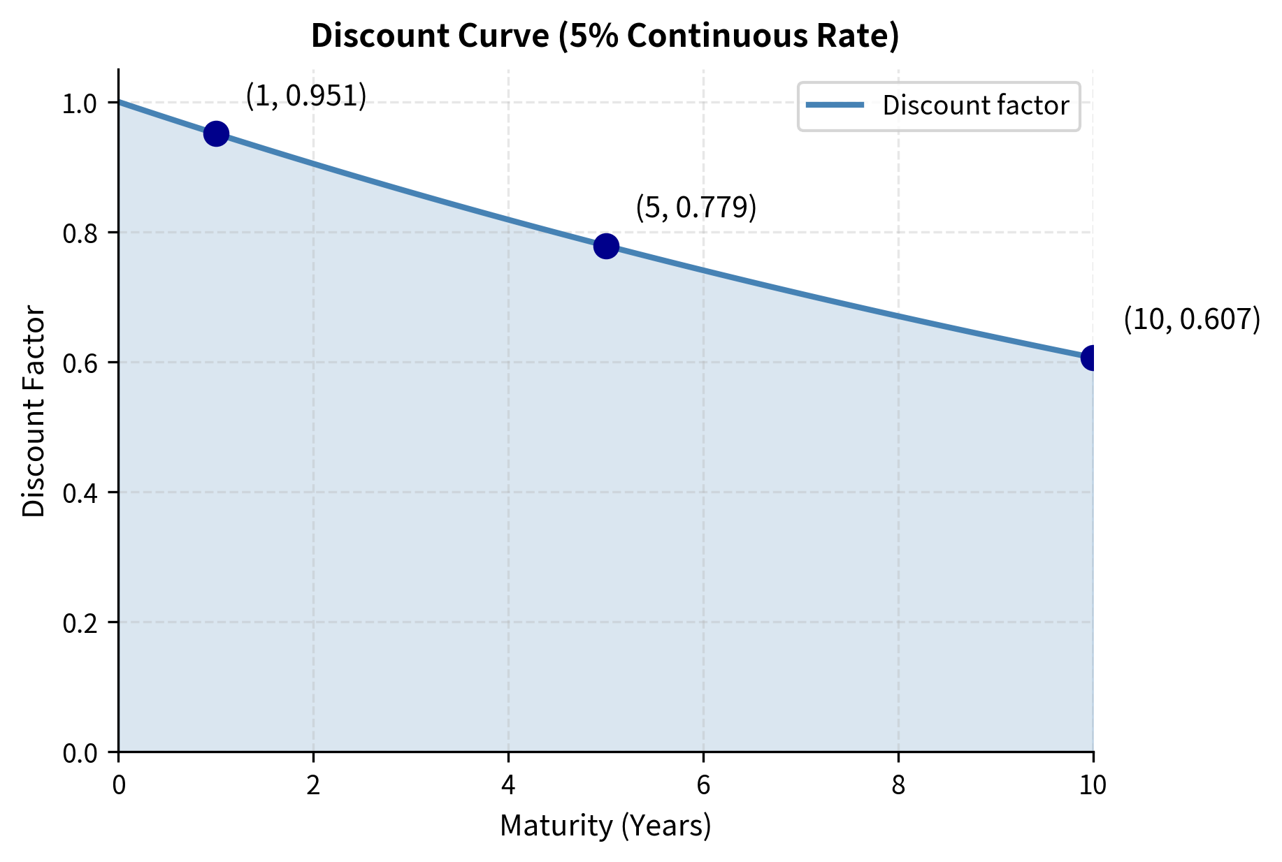
The term $(1 + r)^{-t}$ or $e^{-rt}$ is called the discount factor. It represents the present value of $1 received at time $t$. The discount factor is the "exchange rate" between future dollars and present dollars. If the 5-year discount factor is 0.78, then $1 received in 5 years is worth only $0.78 today, or equivalently, you would need to invest $0.78 today to have $1 in 5 years.

The present value is always less than the future value (assuming positive interest rates). The discount factor tells you what fraction of a future dollar is worth today. At 6% for 5 years, each future dollar is worth about 75 cents today.

In practice, interest rates vary by maturity. Short-term rates may differ substantially from long-term rates. A discount curve (or discount function) maps each maturity to its corresponding discount factor. This curve is a key building block of fixed-income analysis. It contains all the information needed to value any risk-free cash flow occurring at any future date.

The shape of the discount curve reflects market expectations about future interest rates, economic conditions, and risk. A curve that declines steeply indicates either high current rates or expectations of rising rates in the future. A curve that declines slowly suggests lower rates or expectations of falling rates. The entire field of term structure modeling focuses on understanding, constructing, and forecasting this curve.

The discount curve is fundamental to fixed-income analysis. Every bond price, swap valuation, and interest rate derivative depends on the shape of this curve. We will explore term structure modeling in depth in later chapters.

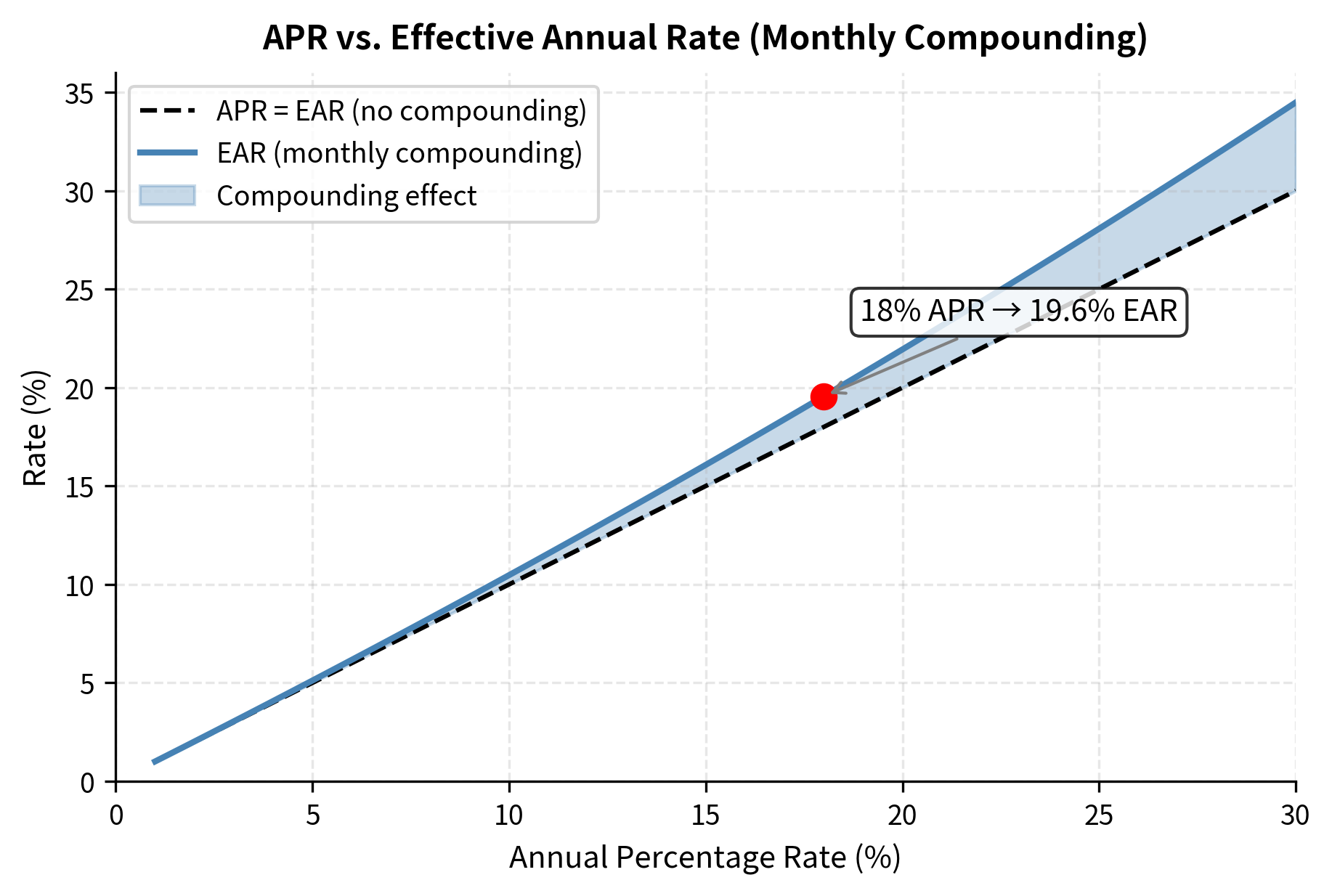
Interest rates in the real world are quoted in various ways, and understanding these quotations is essential for accurate calculations. Two rates that appear identical can imply quite different effective costs or returns depending on how they are quoted. This matters enormously in practice: a credit card advertising "18% APR" is not the same as one offering an "18% effective annual rate," and confusing the two can lead to significant financial errors.

The Annual Percentage Rate (APR) is a nominal rate that does not account for compounding within the year. This is the rate you see advertised for mortgages, credit cards, and loans in many jurisdictions. The APR is essentially a proportional rate. If the monthly rate is 1.5%, the APR is simply 12 × 1.5% = 18%. This makes it easy to calculate and compare, but it understates the true cost of borrowing because it ignores the compounding effect.

The Effective Annual Rate (EAR), also called the Annual Percentage Yield (APY), represents the actual annual return after accounting for compounding:

where:

• $EAR$: effective annual rate (true annual return)
• $APR$: annual percentage rate (nominal/stated rate)
• $n$: number of compounding periods per year
• $(1 + APR/n)^n$: the growth factor over one year with $n$ compounding periods

The formula works by computing what $1 actually grows to over one year: the term $(1 + APR/n)^n$ is the growth factor, representing the final balance after one year per dollar invested. Subtracting 1 converts this growth factor to a rate, expressing the increase as a percentage of the starting amount. The EAR exceeds the APR whenever $n > 1$ because you earn interest on interest within the year. Each period's interest payment begins generating its own returns in subsequent periods.

The gap between EAR and APR grows with both the nominal rate and the compounding frequency. At low rates or with annual compounding, the difference is small. At high rates with frequent compounding, the difference becomes significant. This is why regulators often require lenders to disclose the EAR alongside the APR, giving consumers a more accurate picture of the true cost of borrowing.

A credit card with an 18% APR actually costs 19.56% per year due to monthly compounding. This difference matters significantly for large balances carried over time.

In quantitative finance, we often need to convert between discrete and continuous rates. Market rates are typically quoted with discrete compounding (annual, semi-annual, or monthly), but derivatives models typically work with continuous rates because of their mathematical convenience. These conversions are necessary for moving between the market convention and the modeling convention.

If $r_n$ is the nominal rate compounding $n$ times per year and $r_c$ is the equivalent continuous rate, they must produce the same terminal value over one year:

where:

• $e^{r_c}$: annual growth factor under continuous compounding
• $r_c$: continuously compounded rate
• $r_n$: nominal rate compounding $n$ times per year
• $n$: compounding frequency
• $(1 + r_n/n)^n$: annual growth factor under discrete compounding

This equation states that both rates must produce identical growth factors over one year. They are economically equivalent even though they are expressed differently. Solving for the continuous rate by taking the natural logarithm of both sides:

This formula converts a discretely compounded rate to its continuous equivalent. The logarithm "undoes" the exponential, extracting the continuous rate that achieves the same growth. And converting back by solving for the nominal rate:

This inverse formula takes a continuous rate and finds the discrete rate that produces identical growth. The exponential "undoes" the logarithm, and scaling by $n$ converts from a per-period rate back to an annual nominal rate.

Continuous compounding generates slightly more growth per unit of stated rate. Therefore, a lower continuous rate produces the same terminal value as a higher discretely compounded rate. If you see a continuously compounded rate that looks "too low" compared to market quotes, this difference likely explains it. Continuous rates are always slightly lower than their discrete equivalents.

The continuous rate is slightly lower than the discrete rate because continuous compounding generates slightly more growth for the same rate. This conversion is essential when moving between market-quoted rates and the continuous rates used in derivatives formulas.

Real-world interest calculations must handle fractional years. When interest accrues between two dates that do not span exact years, we need a rule for converting calendar days into a fraction of a year. Different markets use different day count conventions to determine this fraction, and the choice of convention can affect calculated interest amounts, especially for large notional values.

The main conventions are:

• Actual/365: Days between dates divided by 365
• Actual/360: Days between dates divided by 360 (common for money markets)
• 30/360: Assumes 30 days per month, 360 days per year (common for corporate bonds)
• Actual/Actual: Accounts for actual days in each year (used for Treasury bonds)

Each convention has historical origins and practical justifications. Actual/360, for instance, produces larger year fractions than Actual/365 for the same number of days, effectively increasing interest payments. This feature benefits lenders. The 30/360 convention simplifies calculations by assuming uniform months, which was valuable before widespread computer use. Actual/Actual is the most accurate but also the most complex because it requires knowledge of whether any intervening years are leap years.

The same 6-month period produces different year fractions depending on the convention. These differences compound in interest calculations, particularly for large notional amounts. Always verify which convention applies to your specific market and instrument.

Most financial instruments generate multiple cash flows over time. A bond pays coupons. A loan requires monthly payments. A business generates ongoing profits. The time value of money framework extends naturally to value these cash flow streams by treating each cash flow separately and summing the results.

The Net Present Value (NPV) is the sum of all discounted cash flows. It takes each future cash flow, discounts it back to today using the appropriate discount factor, and adds up all these present values. This single number captures the total value of an entire cash flow stream in today's dollars:

where:

• $NPV$: net present value (total value in today's dollars)
• $CF_t$: cash flow occurring at time $t$ (negative for outflows, positive for inflows)
• $r$: discount rate (required rate of return)
• $T$: final period of the cash flow stream
• $(1+r)^{-t}$: discount factor for period $t$
• $\sum_{t=0}^{T}$: summation over all periods from 0 (today) to $T$ (final period)

A positive NPV indicates the investment creates value; a negative NPV indicates it destroys value. NPV answers the question of net benefit in today's dollars by converting all future cash flows to a common time reference. The discount rate $r$ represents your opportunity cost, meaning what you could earn on alternative investments of similar risk. By using this rate to discount future cash flows, you are implicitly comparing the investment to your next best alternative.

The NPV framework embodies a key principle: a dollar of cash flow has different value depending on when it occurs. Early cash flows are worth more than late cash flows, and this difference is precisely captured by the discount factors. The NPV calculation weights each cash flow by its timing, giving appropriate credit to investments that generate returns sooner.

The NPV is positive, indicating the investment generates value at an 8% discount rate. However, NPV is highly sensitive to the discount rate chosen. Let's examine this sensitivity:

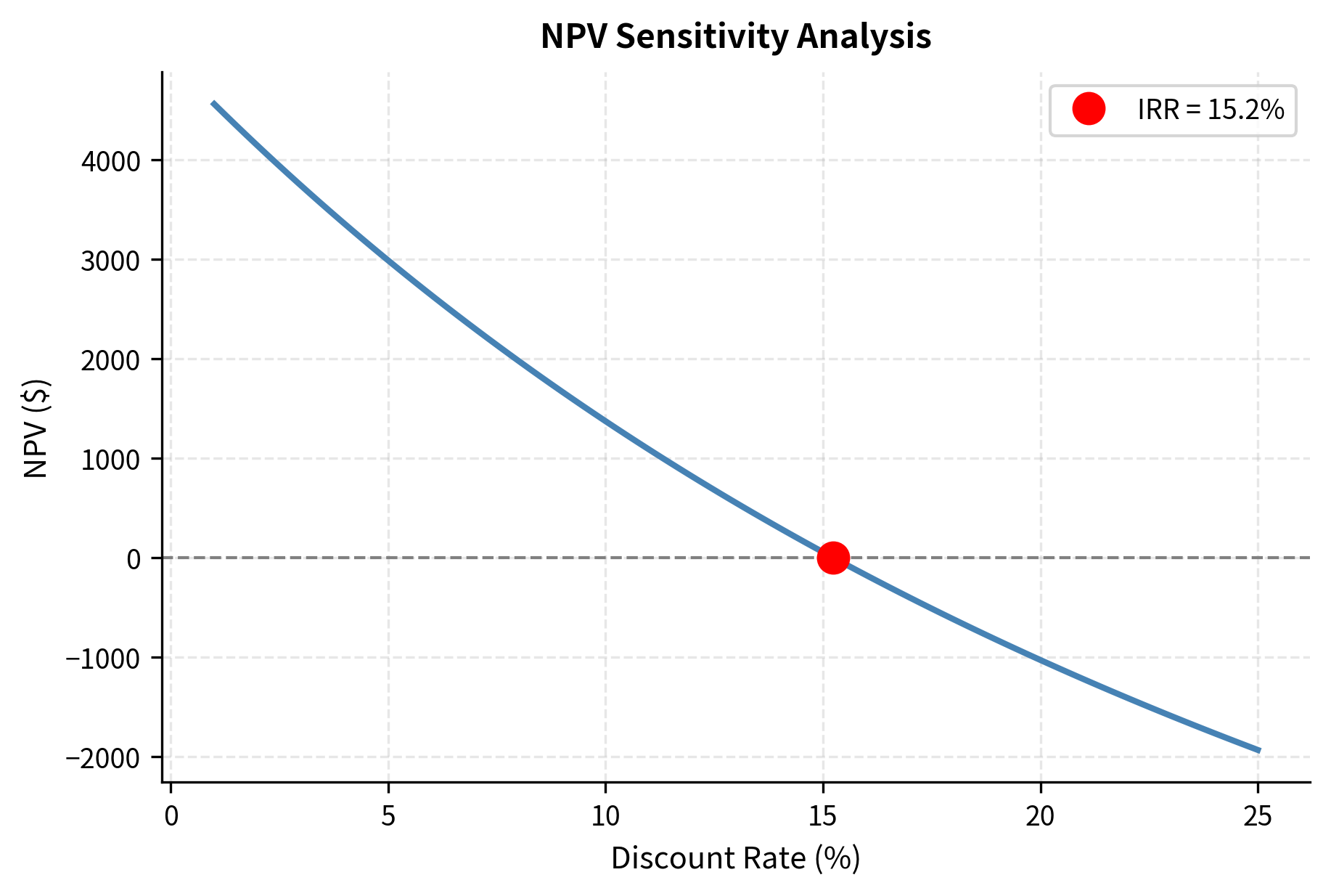
The discount rate where NPV equals zero is called the Internal Rate of Return (IRR). For this investment, the IRR is approximately 15.2%, meaning the investment breaks even at that discount rate.

An annuity is a series of equal payments made at regular intervals. Mortgages, car loans, and many insurance products are structured as annuities. The defining characteristic is regularity: the same amount paid at the same interval for a fixed number of periods. This structure is common enough in finance to merit its own specialized formulas.

Rather than discounting each payment individually and summing, which would require $T$ separate calculations, we can derive a closed-form expression that computes the entire sum at once. The present value of an ordinary annuity (payments at end of each period) is:

where:

• $PV$: present value of the annuity
• $C$: periodic payment amount
• $r$: periodic interest rate (e.g., monthly rate for monthly payments)
• $T$: total number of payment periods
• $\frac{1 - (1+r)^{-T}}{r}$: the annuity factor (present value of $1 per period for $T$ periods)

The annuity formula comes from summing a geometric series of discount factors. The series $1/(1+r) + 1/(1+r)^2 + \ldots + 1/(1+r)^T$ forms a geometric progression with first term $1/(1+r)$ and common ratio $1/(1+r)$. Applying the geometric series formula and simplifying yields the expression above. Rather than computing $C/(1+r) + C/(1+r)^2 + \ldots + C/(1+r)^T$ individually, the closed-form solution captures all terms at once.

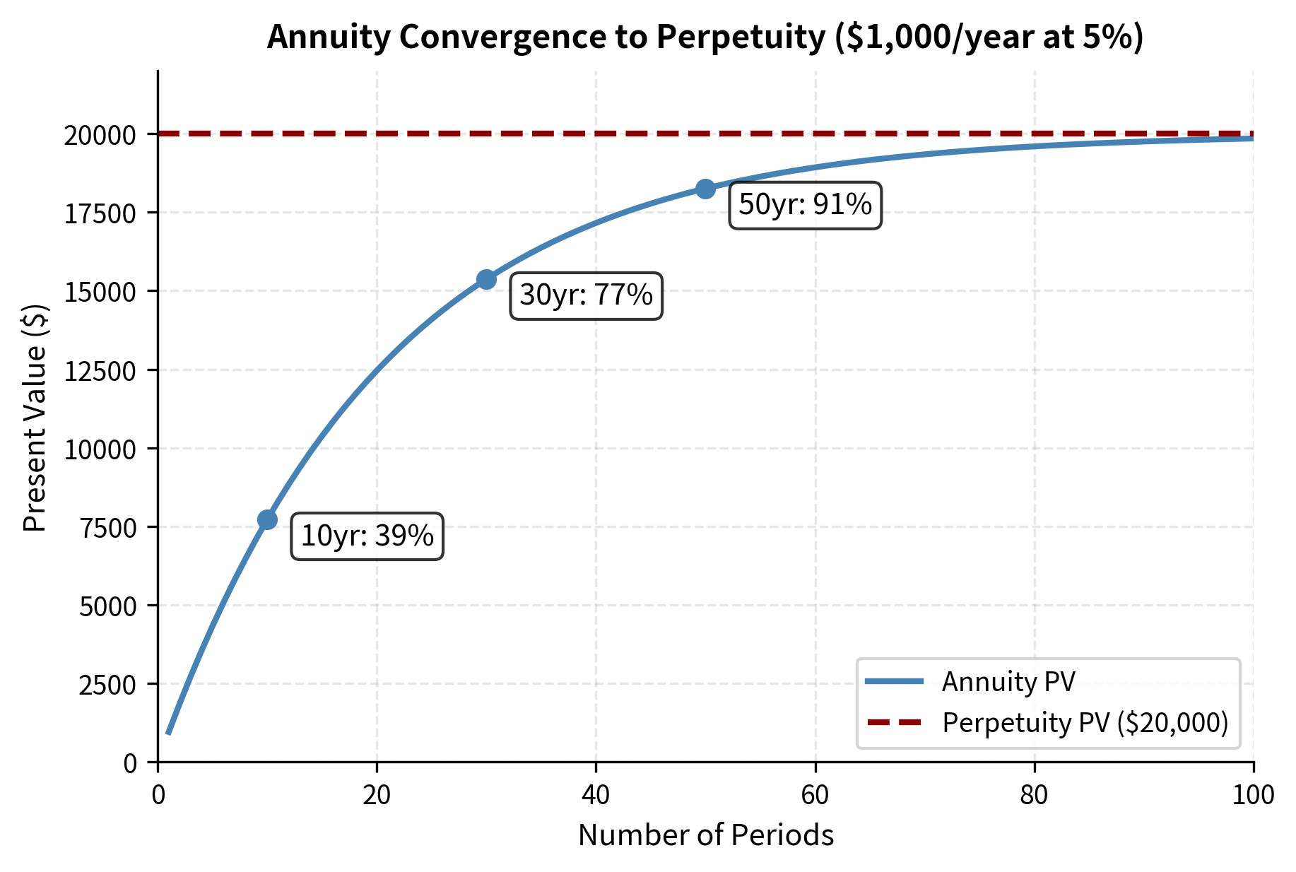
As $T$ increases, the formula approaches $C/r$ (a perpetuity), since very distant payments contribute negligibly to present value. The term $(1+r)^{-T}$ shrinks toward zero, making the numerator approach 1 and the entire factor approach $1/r$. This convergence makes intuitive sense: when payments continue for a very long time, the exact ending point matters less and less.

The term $\frac{1 - (1+r)^{-T}}{r}$ is called the annuity factor. It represents the present value of receiving $1 per period for $T$ periods. This factor depends only on the interest rate and number of periods, not on the payment amount, making it a useful building block. Once you know the annuity factor, you simply multiply by the payment amount to get the present value of any annuity with those characteristics.

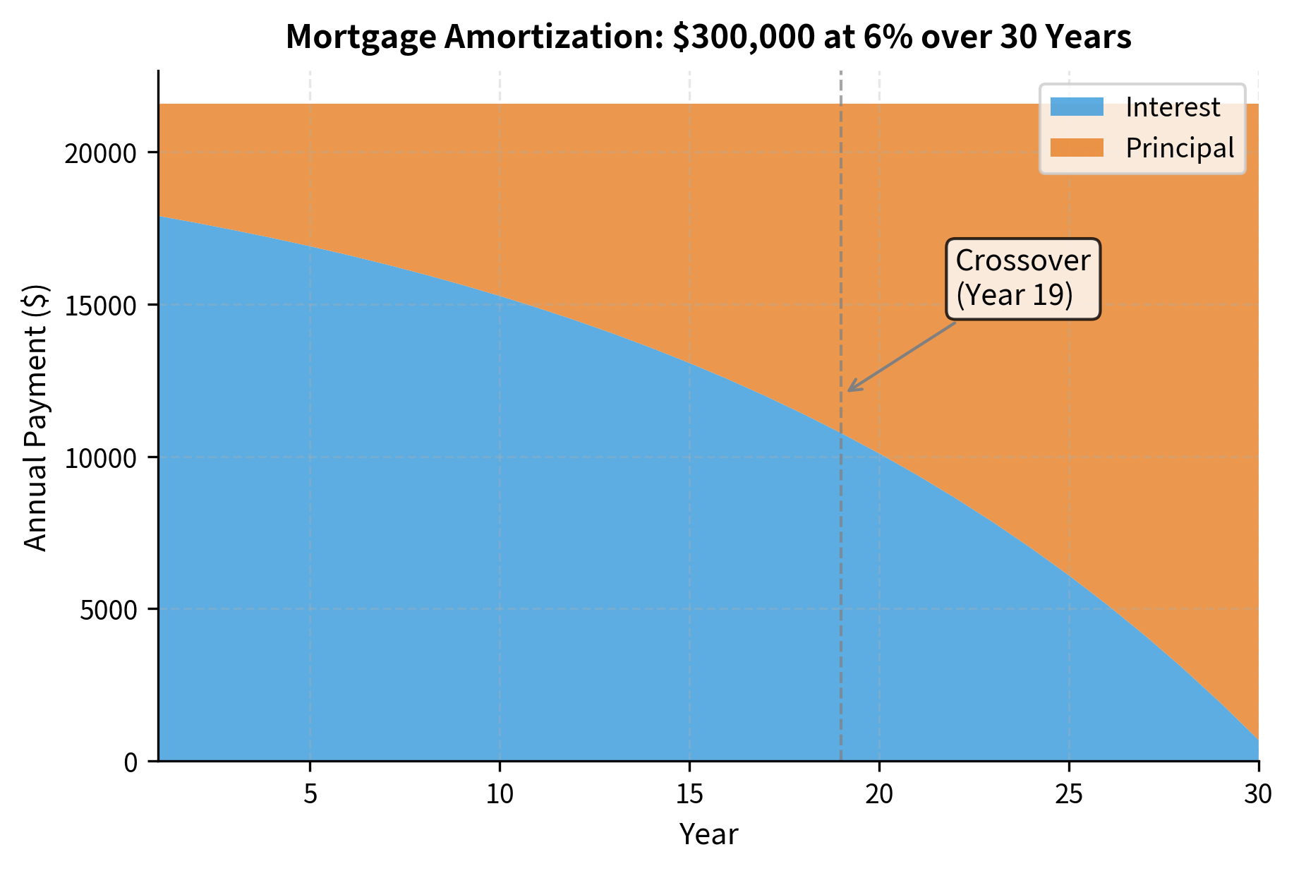
Over 30 years, this borrower pays nearly twice the original loan amount in total. Most of the early payments go toward interest, with principal reduction accelerating over time. This amortization structure has important implications for refinancing decisions.

A perpetuity is an annuity that continues forever. While no financial instrument truly lasts forever, some come close enough, such as British consols and certain endowments, that the perpetuity formula provides a useful approximation.

The present value of a perpetuity is remarkably simple:

where:

• $PV$: present value of the perpetuity
• $C$: constant periodic payment
• $r$: discount rate per period

The present value equals the principal amount that, if invested at rate $r$, would generate exactly $C$ in interest each period forever, leaving the principal intact. If you have $C/r$ dollars earning rate $r$, your interest income is $(C/r) \times r = C$ per period. You can withdraw this interest forever without touching the principal, creating a perpetual income stream of $C$ per period.

This formula emerges from taking the limit of the annuity formula as $T \to \infty$:

As the number of periods grows without bound, the term $(1+r)^{-T}$ vanishes (for any positive $r$), leaving only $C/r$. This mathematical result confirms our intuition: payments occurring in the very distant future contribute almost nothing to present value, so whether the series ends at period 1000 or continues forever makes virtually no difference.

To fund a $50,000 annual scholarship in perpetuity at 4%, the endowment must be $1.25 million. The principal remains intact while only the interest supports the payments.

A growing perpetuity accounts for payments that increase at a constant rate $g$:

where:

• $PV$: present value of the growing perpetuity
• $C$: first payment (occurring one period from now)
• $r$: discount rate per period
• $g$: constant growth rate of payments ($g < r$ required for convergence)
• $r - g$: the "net" discount rate after accounting for growth

Growth partially offsets discounting. When future payments grow, their nominal amounts increase over time, partially counteracting the effect of discounting. For example, if payments grow at 2% while you discount at 5%, the effective discount rate is only 3%. As $g$ approaches $r$, each future payment's present value barely declines, and the sum explodes. Hence the requirement that $r > g$ for the series to converge.

To see why mathematically, consider that the $t$-th payment is $C(1+g)^{t-1}$, and its present value is $C(1+g)^{t-1}/(1+r)^t$. This equals $C/(1+r) \cdot [(1+g)/(1+r)]^{t-1}$. The series converges only when $(1+g)/(1+r) < 1$, which requires $g < r$. If growth equals or exceeds the discount rate, each payment's present value is at least as large as the previous one's, and an infinite sum of non-decreasing positive terms diverges.

This formula is the foundation of the Gordon Growth Model for stock valuation, which we will explore when discussing equity analysis.

Let us apply our time value framework to value a simple bond. A bond is a package of cash flows: periodic coupon payments plus return of principal at maturity. This makes bond valuation a direct application of present value concepts.

Consider a 5-year bond with:

• Face value: $1,000
• Coupon rate: 4% (annual payments)
• Market yield: 5%

The bond's price equals the present value of all future cash flows:

where:

• $P$: bond price (present value of all cash flows)
• $40$: annual coupon payment ($1,000 × 4%)
• $1.05$: one plus the yield (1 + 0.05)
• $1000$: face value returned at maturity
• The first term $\sum_{t=1}^{5} \frac{40}{(1.05)^t}$: present value of the coupon stream (an annuity)
• The second term $\frac{1000}{(1.05)^5}$: present value of the principal repayment

The structure of this formula reflects the two components of a bond's value. The coupon stream is an annuity: five equal payments of $40, one at the end of each year. We can either discount each payment separately or use the annuity formula. The principal repayment is a single lump sum occurring at maturity, which we discount using the basic present value formula. The bond price is simply the sum of these two present values.

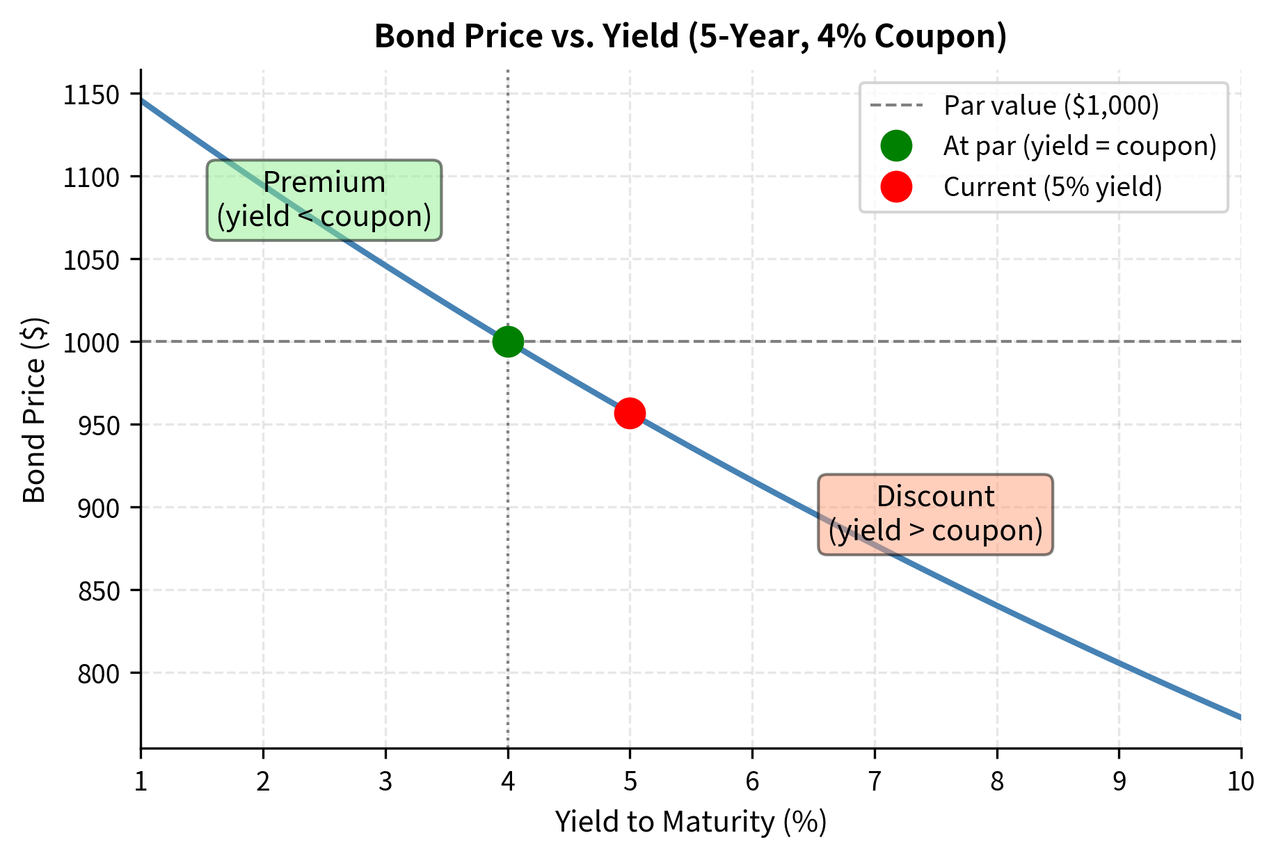
The bond trades at a discount ($956.71 vs. $1,000 face) because its 4% coupon is below the 5% market yield. Investors require compensation for accepting below-market coupons, which comes in the form of a lower price.

Let's visualize how the bond's cash flows contribute to its price:

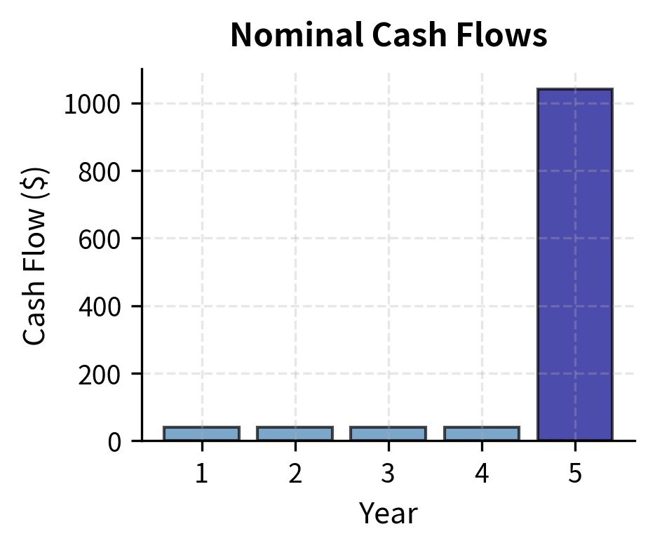
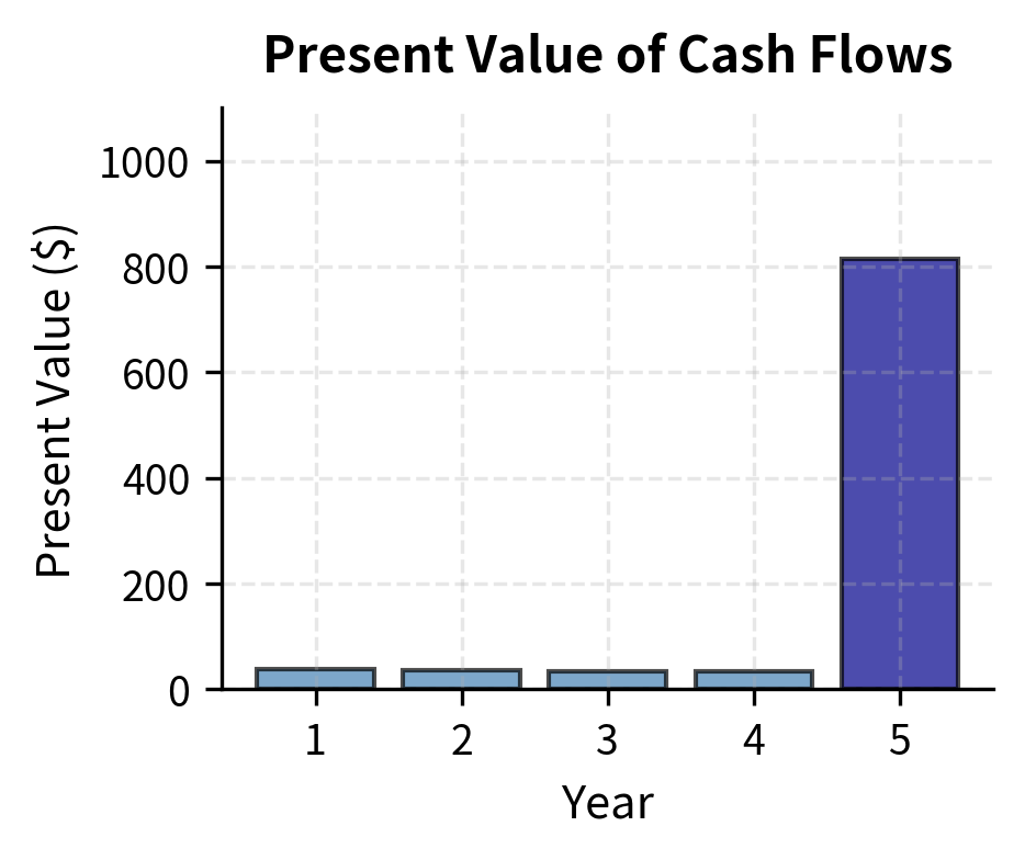
The final cash flow of $1,040 (coupon plus principal) accounts for the bulk of the bond's value, but its contribution is substantially reduced when discounted back five years.

The time value of money framework is powerful but rests on assumptions that may not hold in practice. Understanding these limitations helps you apply the framework appropriately and recognize when more sophisticated approaches are needed.

The most significant limitation is the assumption of a constant, known discount rate. In reality, interest rates vary over time, differ across maturities (the term structure), and contain uncertainty about future values. A bond's yield is actually a single rate that equates the present value calculation to the market price. This yield is a convenient fiction rather than a fundamental constant. When valuing complex instruments or long-dated cash flows, using a single rate obscures important term structure effects. Proper fixed-income analysis requires working with the full yield curve, extracting zero-coupon rates, and often modeling rate dynamics stochastically.

Selecting the appropriate discount rate is one of the most important and difficult judgments in any valuation exercise. For risk-free cash flows like Treasury bonds, the choice is relatively straightforward. For corporate bonds, project cash flows, or equity valuations, the discount rate must reflect credit risk, liquidity risk, and business risk. Small changes in the discount rate produce large changes in present value, particularly for long-duration cash flows. This sensitivity means valuation is inherently uncertain, and practitioners should always examine how their conclusions change under different discount rate assumptions.

Day count conventions, compounding frequencies, and accrued interest calculations introduce complexity that can cause errors if handled incorrectly. Different markets quote rates differently. The same nominal rate under different conventions produces different cash flows. Professional fixed-income systems maintain detailed convention databases, and any serious quantitative work requires careful attention to these details.

Finally, the framework assumes cash flows are known with certainty. Most real-world cash flows are uncertain: companies may default, projects may underperform, and prepayments may occur unexpectedly. Extending the basic framework to handle uncertainty requires probability theory, expected value calculations, and risk adjustment. We address these topics in subsequent chapters.

This chapter covered the core concepts of time value of money and interest rates used throughout quantitative finance. You learned that money has time value because it can be invested, inflation erodes purchasing power, and future payments carry uncertainty.

We developed the mathematics of compounding, progressing from simple interest through discrete compounding to the continuous compounding framework preferred in derivatives pricing. You now understand how to move between present and future values using discount factors, and how to convert between different rate quotations (APR, EAR, continuous rates) and day count conventions.

For valuing cash flow streams, you learned to calculate net present value, recognize when the annuity and perpetuity formulas apply, and understand the sensitivity of valuations to discount rate assumptions. The bond valuation example demonstrated how these tools combine in practice.

The key formulas to remember are:

• Future value (continuous): $FV = Pe^{rt}$
• Present value (continuous): $PV = FV \cdot e^{-rt}$
• Annuity PV: $PV = C \cdot \frac{1-(1+r)^{-T}}{r}$
• Perpetuity PV: $PV = C/r$

These building blocks appear throughout the book as we work with more complex instruments. The next chapter examines how interest rates across different maturities form term structures, and how we extract the discount factors needed for precise valuation from market prices.

Ready to test your understanding? Take this quick quiz to reinforce what you've learned about the time value of money and interest rates.