

Learn policy gradient theory for language model alignment. Master the REINFORCE algorithm, variance reduction with baselines, and foundations for PPO.

This article is part of the free-to-read Language AI Handbook
Choose your expertise level to adjust how many terms are explained. Beginners see more tooltips, experts see fewer to maintain reading flow. Hover over underlined terms for instant definitions.
Policy Gradient Methods
With a trained reward model that captures human preferences, we face a fundamental challenge: how do we use this reward signal to actually improve our language model? The reward model tells us whether a complete generated response is good or bad, but our language model makes decisions token by token. We need a way to propagate that final reward signal back to influence all the individual token choices that led to it.
This is where reinforcement learning enters the picture. Unlike supervised learning, where we have explicit targets for each prediction, reinforcement learning handles the credit assignment problem: determining how much each action contributed to the eventual outcome. Policy gradient methods provide a mathematically principled framework for optimizing a model's behavior based on sparse, delayed reward signals.
In this chapter, we'll develop the theory behind policy gradients from first principles, derive the key mathematical results that make training possible, and implement the REINFORCE algorithm. This foundation is essential for understanding PPO and the complete RLHF pipeline that follows in subsequent chapters.
Language Models as Policies
In reinforcement learning terminology, a policy is a function that maps states to actions. For language models, this mapping has a natural interpretation that becomes clear once we examine how text generation actually works. When you ask a language model to complete a sentence, it doesn't produce the entire response instantaneously. Instead, it generates one token at a time, each choice depending on everything that came before. This sequential decision-making process is precisely what reinforcement learning was designed to handle.
A policy is a probability distribution over actions given state , parameterized by . In language models, the policy is the model itself: given a context (state), it produces a probability distribution over the next token (action).
To understand why this framing is so powerful, consider what happens during text generation. The model receives a prompt, which establishes the initial context. Based on this context, the model must decide which token to produce first. This decision changes the context, as the newly generated token becomes part of the history. The model then faces a new decision: given the original prompt plus the first generated token, what should the second token be? This process continues, with each token choice altering the state and presenting a fresh decision problem.
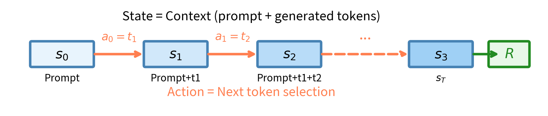
When a language model generates text, it's acting as a policy:
- State : The current context, consisting of the prompt plus all tokens generated so far
- Action : The next token to generate
- Policy : The probability the model assigns to token given context
This framing reveals why language model alignment is fundamentally a reinforcement learning problem. At each timestep, the model takes an action (selects a token), the state changes (the context grows), and eventually the complete sequence receives a reward from our reward model. The challenge is learning which tokens led to that reward. Unlike a game where individual moves might receive immediate feedback, language generation only reveals whether the response was good or bad after the entire sequence is complete. This delayed reward structure is exactly the scenario where reinforcement learning excels.
The model's parameters define the policy. Our goal is to adjust these parameters so that the model generates responses that receive high rewards. This means we need to find parameter values that make high-reward sequences more probable and low-reward sequences less probable. The question is: how do we know which direction to adjust the parameters?
The Objective Function
To optimize our policy, we need a clear objective. In RLHF, we want to maximize the expected reward over all possible responses the model might generate. This expectation is crucial because language generation is inherently stochastic. The same prompt can lead to many different responses depending on which tokens get sampled at each step. Some responses will be excellent, others will be mediocre, and still others will be poor. We want to tune the model so that, on average, it produces responses that receive high rewards.
Given a prompt , the model generates a response by sampling tokens according to its policy. The reward model then scores the complete response, giving us . Our objective:
where:
- : the objective function we want to maximize
- : the parameters of the language model
- : the expectation over sequences sampled from the policy
- : the policy (language model) distribution conditioned on prompt
- : the reward scalar for the generated response
This expectation is taken over all possible responses the model could generate. Some responses will be excellent (high reward), others mediocre, others poor. The expectation weights each by its probability under the current policy. This weighting is important: if the model rarely generates a particular response, that response contributes little to the expected value, even if it happens to have high reward.
We can expand this using the probability of generating the complete sequence:
- : summation over all possible output sequences in the vocabulary
- : probability of generating sequence given prompt
- : reward for the specific sequence
The probability represents the likelihood of generating the entire response . It is computed as the product of individual token probabilities:
where:
- : the length of the generated sequence
- : the token generated at timestep
- : the history of tokens generated before step
- : probability of the next token given context
This autoregressive factorization, which we've seen throughout our discussion of language models, connects the policy formulation directly to how transformers and LSTMs actually generate text. Each factor in the product corresponds to one step of the generation process, one call to the model's forward function, one decision about which token to emit next. The full sequence probability is simply the product of all these individual decisions.
The Policy Gradient Theorem
Here's the core challenge: how do we compute ? We need this gradient to update our parameters via gradient ascent, but the expectation involves sampling from the policy itself, which depends on . This creates a circular dependency that seems difficult to resolve. The gradient depends on how changing affects which sequences get sampled, but sampling is a discrete, non-differentiable operation. We cannot simply backpropagate through the sampling process the way we would through a continuous neural network layer.
The policy gradient theorem provides an elegant solution to this problem. Rather than trying to differentiate through sampling directly, it rewrites the gradient in a form that we can estimate using samples from the current policy. The key insight is that we can express the gradient of an expectation in terms of an expectation of gradients, which is something we can actually compute.
Let's derive the policy gradient step by step. Starting with our objective:
The gradient with respect to :
Reward doesn't depend on (it comes from a fixed reward model), so only the policy probability is differentiated. This is an important observation: the reward model is frozen during policy optimization, so its output is just a scalar that multiplies the gradient.
Now we apply a crucial mathematical trick called the log-derivative trick. This technique appears throughout machine learning and statistics whenever we need to compute gradients of expectations. The core idea is to introduce a logarithm and then remove it in a way that reveals a useful structure. Starting from the identity:
We recognize that:
This follows from the chain rule: . The logarithm converts a multiplicative relationship into an additive one, which will prove extremely useful when we deal with sequence probabilities that are products of many terms.
Substituting back:
A sum over all possible sequences weighted by their probabilities is exactly an expectation:
- : gradient of the objective function w.r.t. parameters
- : gradient of the log-probability of the sequence (the "score function")
- : the reward acting as a scalar weight
This is the policy gradient theorem for our setting. It tells us something remarkable: to compute the gradient of expected reward, we can sample sequences from our policy, compute the gradient of their log-probabilities, and multiply by their rewards. The score function points in the direction that would increase the probability of sequence . Multiplying by the reward scales this direction: high rewards give large positive contributions, low rewards give small or negative contributions.
The gradient of expected reward:
where:
- : gradient of the objective function
- : expectation over sampled sequences
- : gradient of the log-probability (score function)
- : reward of the sampled sequence
This transforms an intractable sum over all possible sequences into a tractable Monte Carlo estimate using samples from the policy.
The transformation from an intractable sum to a Monte Carlo estimate is the key practical insight. We cannot enumerate all possible sequences; for even modest vocabulary sizes and sequence lengths, this would involve more sequences than atoms in the universe. But we can sample sequences from our policy, and the policy gradient theorem tells us that averaging over these samples gives us an unbiased estimate of the true gradient.
From Sequences to Tokens
For language models, we need to express the log-probability of an entire sequence in terms of individual tokens. This connection is essential because our models compute token-level probabilities, not sequence-level probabilities directly. Fortunately, the autoregressive structure of language models makes this straightforward. Using the autoregressive factorization:
where:
- : sum over all timesteps in the sequence
- : log-probability of the specific token given context
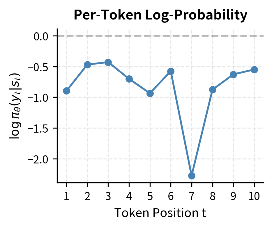
The logarithm converts the product of probabilities into a sum of log-probabilities. This is where the log-derivative trick pays off: instead of dealing with products of many small numbers (which can underflow numerically), we work with sums of log-probabilities, which are much more stable.
Each term is simply the log-softmax output of our model at position , evaluated at the token that was actually selected. This is exactly what we compute during the forward pass. When the model processes a sequence, it produces logits for every position, and applying log-softmax gives us log-probabilities. To compute the log-probability of a specific token choice, we simply index into this log-probability vector at the chosen token's index.
The gradient of the full sequence log-probability is then:
where:
- : the state (context) at timestep , equivalent to
- : gradient of the log-probability for a single token
This sum of gradients follows from the linearity of differentiation. The gradient of a sum is the sum of gradients. Each term in the sum corresponds to one token's contribution to the overall sequence probability.
Putting this together, the policy gradient becomes:
where:
- : the accumulated gradient from all tokens in the sequence
- : the final reward, which scales the gradient of every token choice
The same reward multiplies every token's gradient. This is the key insight: even though we only receive reward at the end, it propagates back to influence all token choices. Every token that contributed to the response receives the same credit or blame for the final outcome. This is both a strength and a weakness of the basic approach. It allows learning from sparse rewards, but it doesn't distinguish between tokens that were crucial for the reward and tokens that were irrelevant.
The REINFORCE Algorithm
The policy gradient theorem gives us a theoretical result. REINFORCE (also called Monte Carlo policy gradient) is the algorithm that turns this theory into practice through Monte Carlo estimation. The name comes from the idea that we "reinforce" behaviors that lead to good outcomes: when a sequence receives high reward, we reinforce the probability of generating that exact sequence.
The algorithm is elegantly simple:
- Sample a complete sequence from the current policy
- Compute the reward for that sequence
- For each token, compute
- Sum these gradients and update parameters
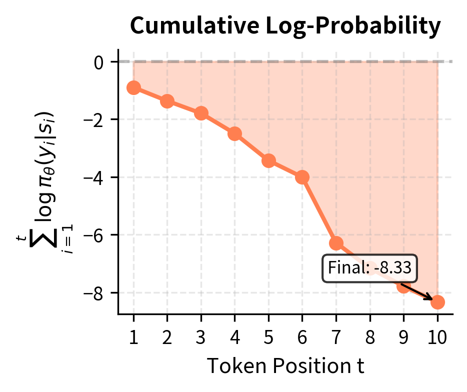
Let's trace through a concrete example to build intuition. Suppose our model generates a three-token response with probabilities 0.3, 0.5, and 0.2, receiving a reward of +1. The log-probability of the sequence is:
where:
- , , etc.: log-probabilities of individual tokens
- : the cumulative log-probability of the complete sequence
Notice that the log-probability is negative, which is always the case since probabilities are between 0 and 1. A log-probability of -3.91 corresponds to a probability of about 0.02, which makes sense: it's the product .
The REINFORCE gradient update uses the term:
where:
- : the gradient contribution from this single sample
- : the reward ()
- : the direction in parameter space that increases the log-probability (which is in this example)
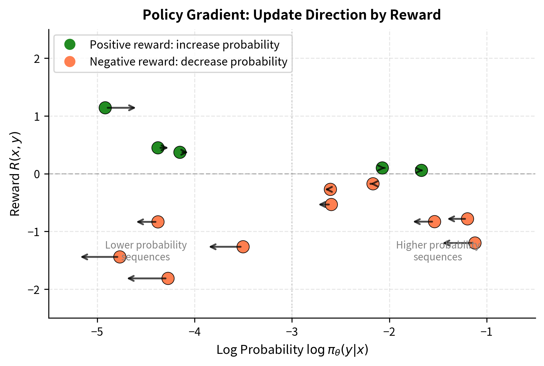
This gradient pushes the model to increase the probability of generating this exact sequence. If the reward had been instead, the gradient would push in the opposite direction, making this sequence less likely. The reward acts as a scaling factor that determines both the magnitude and direction of the update.
The intuition is clear: REINFORCE increases the probability of sequences that receive high rewards and decreases the probability of sequences that receive low rewards. Over many updates, the policy gradually shifts to favor the kinds of responses that the reward model prefers. This is the essence of learning from rewards: try things, see what works, do more of what works.
The Variance Problem
REINFORCE has a critical weakness: extremely high variance in its gradient estimates. This variance comes from several sources:
- Sampling variance: We estimate an expectation using a single sample (or small batch). Different samples from the same policy can have wildly different rewards. Consider a prompt where some responses are brilliant (reward +10) and others are terrible (reward -10), but most are mediocre (reward near 0). If we happen to sample one of the rare brilliant responses, we get a huge positive gradient. If we sample a terrible one, we get a huge negative gradient. The expected gradient might be small and stable, but individual estimates can be orders of magnitude larger.
- Reward magnitude: Large rewards amplify gradient noise. A reward of 100 versus 0.1 changes gradient magnitudes by a factor of 1000. If the reward scale varies across prompts or across training, the gradient scale varies too. This makes it hard to choose a stable learning rate.
- Long sequences: With more tokens, there's more opportunity for randomness in the sampling process. Each token choice is stochastic, and these random choices compound. The same prompt can lead to vastly different sequences purely due to sampling randomness early in generation.
To see why this matters, consider the policy gradient:
- : the batch size (number of sampled sequences)
- : the -th sampled sequence in the batch
- : the reward for the -th sequence
If rewards vary from -10 to +10, these gradient estimates will swing wildly between updates. The model may get pushed in completely different directions on consecutive batches, even with the same prompt, simply due to sampling randomness. This creates a noisy optimization landscape where progress is slow and inconsistent.
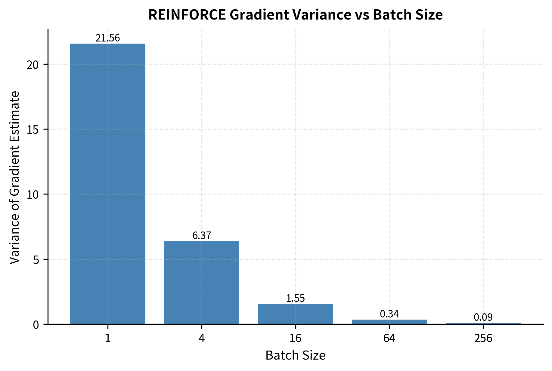
The variance decreases at rate with batch size , but this means we need exponentially more samples to achieve linear improvements in stability. This is fundamentally inefficient. To reduce variance by a factor of 10, we need 10 times more samples. To reduce it by a factor of 100, we need 100 times more samples. For large language models where each sample is expensive to generate, this sample inefficiency becomes a serious practical barrier.
Variance Reduction with Baselines
The key insight for reducing variance comes from a useful property of the policy gradient: subtracting any constant from the reward doesn't change the expected gradient, but it can dramatically reduce variance. This property allows us to center the rewards around zero without introducing any bias into our gradient estimates.
Consider adding a baseline to our gradient estimator:
- : a baseline value (constant w.r.t. the action )
- : the "centered" reward, reducing variance
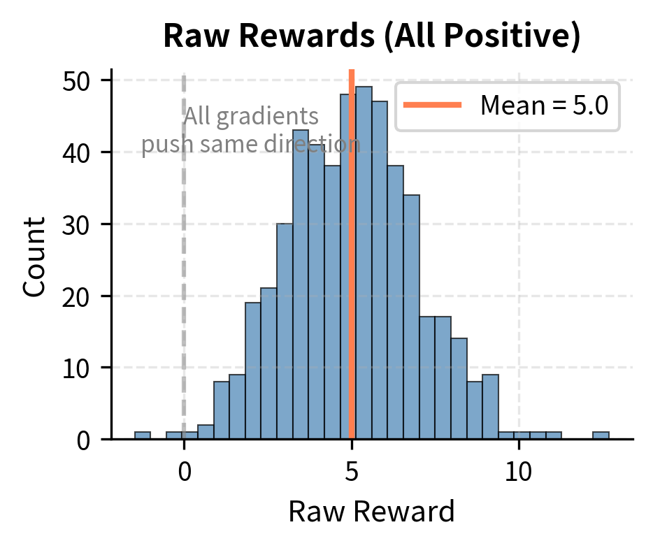
Why does centering help? Consider the extreme case where all rewards are positive, say ranging from +5 to +15. Without a baseline, every gradient update pushes to increase the probability of all sampled sequences. The model learns slowly because it's receiving mixed signals: "increase this sequence, increase that sequence too, increase everything." With a baseline of 10, rewards become -5 to +5. Now the gradient clearly distinguishes: "increase sequences above the baseline, decrease sequences below it." This clearer signal leads to faster learning.
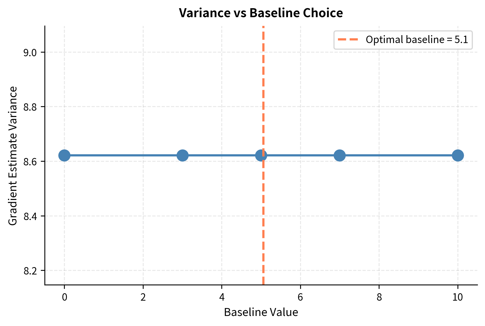
To verify this doesn't change the expected gradient, we check that the baseline term contributes zero in expectation:
The expectation of the score function is zero:
This result shows that the score function always has zero mean. This is because the score function measures how changing parameters affects the log-probability of different outcomes, and these effects must balance out since probabilities always sum to one. Increasing the probability of some outcomes necessarily decreases the probability of others.
This result implies that we can subtract any baseline without introducing bias. The question becomes: what baseline minimizes variance?
The optimal baseline turns out to be the expected reward:
where:
- the variance-minimizing baseline value
- : the expected reward under the current policy (often approximated by a value function )
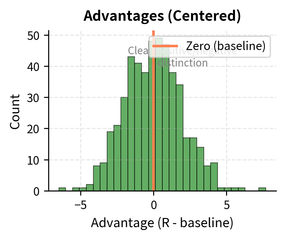
This is called a value baseline, and in practice we often estimate it with a learned value function. With this baseline, the quantity becomes the advantage: how much better (or worse) this specific sequence is compared to what we expect on average. The advantage is positive when a response exceeds expectations and negative when it falls short.
The advantage measures how much better a response is compared to the expected reward from the current policy:
where:
- : the advantage score
- : the reward for sequence
- : the value function estimating expected reward
Positive advantage means better than average; negative means worse.
The advantage has a natural interpretation: it measures how "surprising" a reward is relative to what we expected. A response with advantage +5 did much better than typical; one with advantage -3 did worse. By training on advantages rather than raw rewards, we give the model clearer information about which responses are actually good.
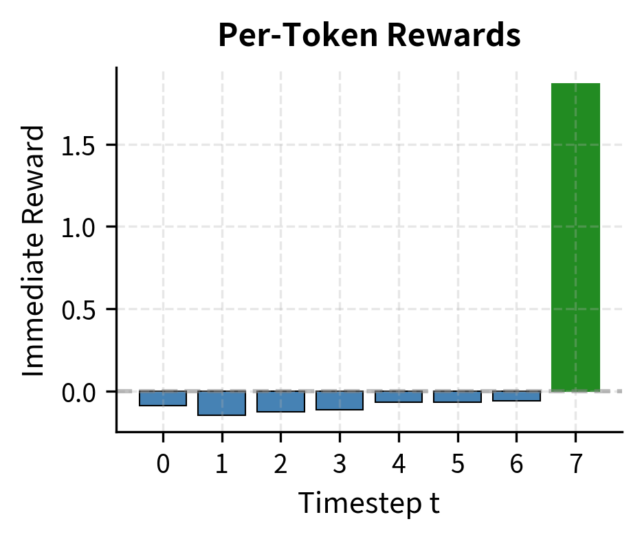
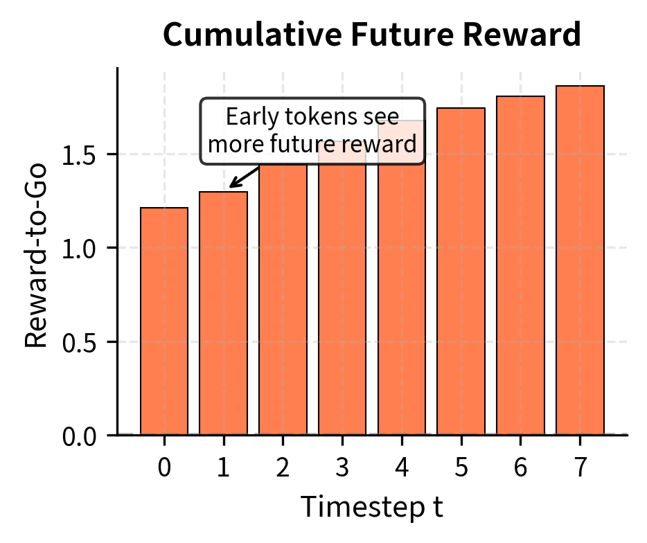
Reward-to-Go
Another variance reduction technique acknowledges that actions only affect future rewards, not past ones. This is a causal observation: a decision made at time cannot retroactively change what happened at time . Yet in basic REINFORCE, we multiply every token's gradient by the full sequence reward, even though early tokens cannot have influenced rewards that were "already determined" by the time they were generated.
Instead of multiplying each token's gradient by the total reward, we can use only the rewards that could have been influenced by that action. This is called the reward-to-go formulation. If we only receive reward at the end of the sequence, the reward-to-go at each timestep is the same as the final reward. However, if we were to introduce intermediate rewards (for example, per-token penalties for certain words), the reward-to-go at step would be:
where:
- : reward-to-go from timestep
- : immediate reward received at timestep
The sum starts at the current timestep and runs to the end of the sequence . This captures only the future rewards, ignoring any rewards that occurred before the action was taken.
The policy gradient becomes:
where:
- : expectation over sequences sampled from the policy
- : the token generated at timestep (previously denoted as action )
- : the cumulative reward from time onwards (reward-to-go), ignoring past rewards
This doesn't change the expected gradient (the proof is similar to the baseline case) but reduces variance by removing terms that contribute only noise. The intuition is that past rewards add randomness without providing useful signal about the current action. By excluding them, we get cleaner gradient estimates.
In the typical RLHF setup where reward is only given at the end, reward-to-go equals the final reward at all timesteps. However, this structure becomes important when we add auxiliary rewards or penalties, such as the KL divergence penalty we'll introduce in subsequent chapters. That penalty applies at each token, creating a richer reward structure where reward-to-go provides meaningful variance reduction.
Complete Implementation
Let's put everything together into a complete REINFORCE implementation with baseline and proper training loop.
Now let's test this with a simple reward function that encourages shorter sequences:
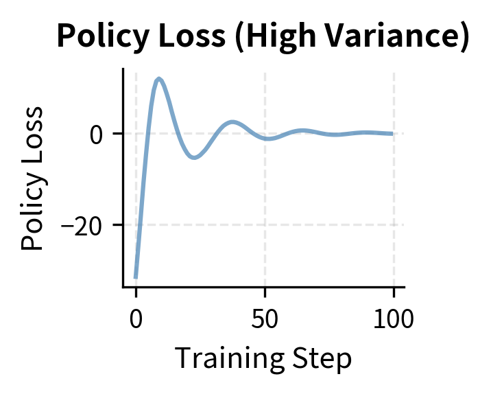
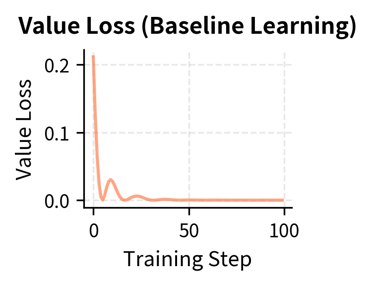
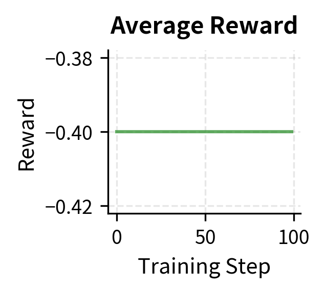
The plots reveal the characteristic noisiness of REINFORCE training. While the value network learns to predict expected rewards (value loss decreases), the policy loss remains highly variable. This variance is the primary motivation for more sophisticated algorithms.
Additional Variance Reduction Techniques
Beyond baselines and reward-to-go, several additional techniques help control variance in practice.
Reward normalization standardizes rewards across a batch to have zero mean and unit variance:
This prevents large reward magnitudes from causing gradient explosions while preserving the relative ordering of rewards.
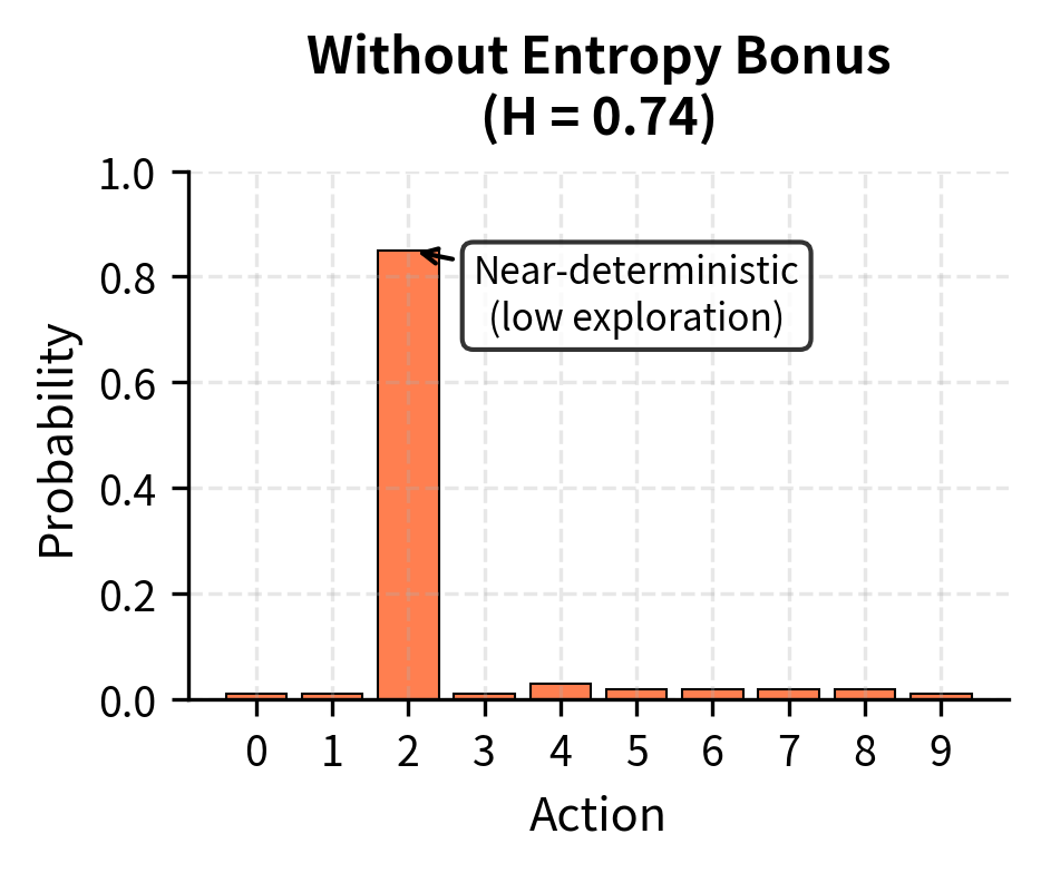
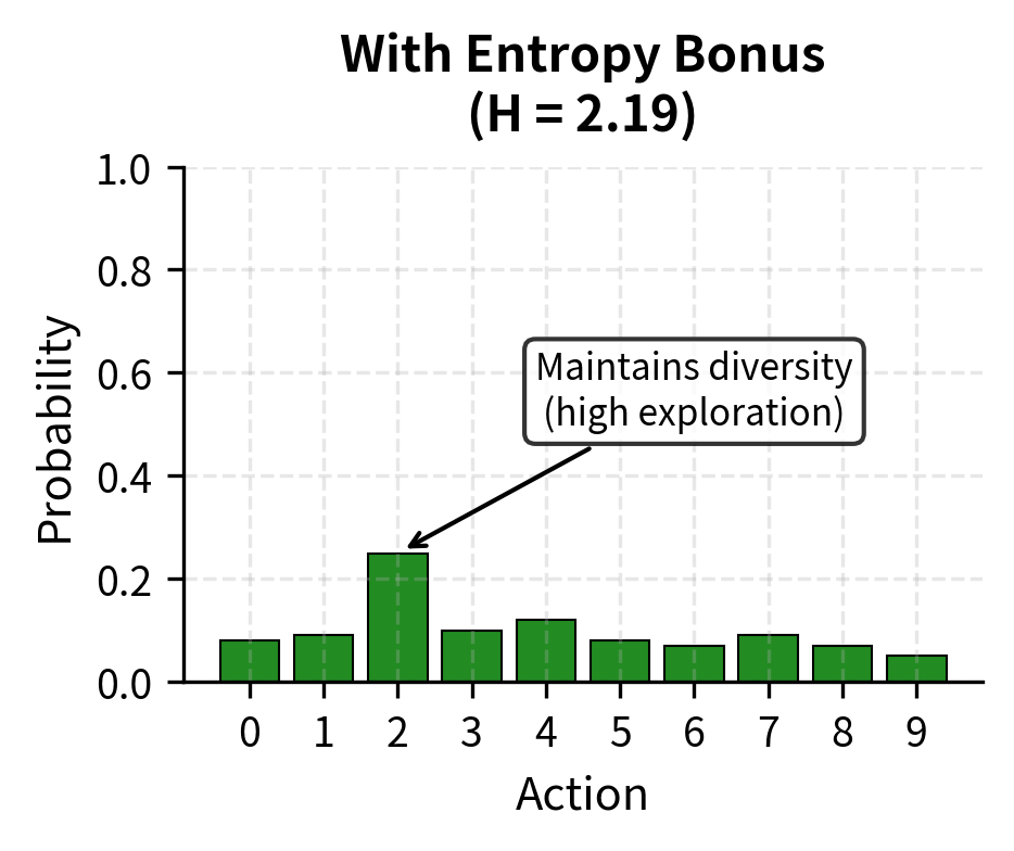
Entropy regularization adds a bonus for maintaining policy entropy, preventing premature convergence to deterministic behavior:
High entropy means the policy is exploring diverse actions; low entropy means it's becoming deterministic. The entropy bonus encourages continued exploration, which can help escape local optima.
Gradient clipping limits the magnitude of gradient updates:
As we discussed in Part VII, gradient clipping prevents individual updates from being too large, which is especially important given REINFORCE's high variance.
Limitations and Practical Challenges
REINFORCE, while theoretically elegant, has significant practical limitations that make it challenging for training large language models:
- Sample efficiency: REINFORCE requires many samples to get reliable gradient estimates. For large language models generating hundreds of tokens, each sample is expensive: it requires a full forward pass and potentially a reward model evaluation. Training can require millions of samples, which becomes prohibitively expensive with models that have billions of parameters.
- Credit assignment: The credit assignment problem is only partially solved. While the policy gradient attributes reward to all tokens equally, this isn't always appropriate. A response might be mostly good with one problematic sentence, yet every token receives the same reward signal. More sophisticated algorithms like actor-critic methods (which we'll see with PPO) attempt to provide finer-grained credit assignment.
- Update stability: REINFORCE provides no guarantees about the size of policy updates. A lucky high-reward sample can push the policy dramatically in one direction, only for the next batch to push it back. This oscillation wastes computation and can destabilize training. The PPO algorithm, covered in the next chapter, directly addresses this by constraining how much the policy can change per update.
Despite these limitations, REINFORCE remains important as the foundation for understanding more sophisticated algorithms. PPO, TRPO, and other policy gradient methods all build on the same core gradient estimator. Understanding REINFORCE's mechanics and failure modes helps explain why those algorithms make the design choices they do.
Summary
Policy gradient methods provide the mathematical foundation for optimizing language models using reward signals. The key insights from this chapter are:
- Language models are policies. The autoregressive generation process naturally maps to the RL framework: states are contexts, actions are tokens, and the policy is the model's token probability distribution.
- The policy gradient theorem enables optimization. By rewriting the gradient as , we transform an intractable sum into a Monte Carlo estimate that we can compute from samples.
- REINFORCE is simple but high-variance. The basic algorithm just samples sequences, computes their rewards, and updates parameters in proportion to . This works but requires many samples for stable estimates.
- Baselines reduce variance without introducing bias. Subtracting a baseline from rewards yields the same expected gradient but lower variance. The optimal baseline is the expected reward, leading to the advantage formulation .
- Additional techniques help in practice. Reward normalization, entropy regularization, and gradient clipping all contribute to more stable training.
The variance problem with REINFORCE motivates the development of more sophisticated algorithms. In the next chapter, we'll see how Proximal Policy Optimization (PPO) addresses these issues by constraining policy updates and using more careful gradient estimation, making RL-based alignment practical for production language models.
Quiz
Ready to test your understanding? Take this quick quiz to reinforce what you've learned about policy gradient methods and the REINFORCE algorithm.

Comments