PPO Algorithm: Proximal Policy Optimization for Stable RL

In the previous chapter, we explored policy gradient methods and saw how REINFORCE directly optimizes a policy by following the gradient of expected reward. While mathematically elegant, vanilla policy gradients have a critical practical limitation: they are notoriously unstable during training. A single large gradient update can catastrophically degrade policy performance, making recovery difficult. This instability motivates better algorithms. Proximal Policy Optimization (PPO), introduced by Schulman et al. in 2017, addresses this instability through a simple mechanism: it clips the objective function to prevent updates that change the policy too drastically.

PPO is the standard algorithm for reinforcement learning from human feedback in language models because of its stability, sample efficiency, and implementation simplicity. Understanding PPO's mechanics helps you fine-tune language models to follow human preferences.

Recall that the policy gradient takes the form:

To understand why this formula creates practical difficulties, examine what each component contributes:

• $\nabla_\theta J(\theta)$: the gradient of the expected cumulative reward with respect to policy parameters, showing the direction to adjust parameters to increase expected reward
• $\mathbb{E}_{\tau \sim \pi_\theta}$: expectation over trajectories sampled from the current policy $\pi_\theta$
• $\theta$: parameters of the policy network that we are optimizing
• $J(\theta)$: the expected cumulative reward under policy $\pi_\theta$
• $\tau$: a trajectory (sequence of states and actions) sampled from the current policy
• $\pi_\theta(a_t | s_t)$: the probability of taking action $a_t$ in state $s_t$ under the current policy
• $T$: the time horizon, the length of the episode
• $A_t$: the advantage function at time $t$, estimating how much better action $a_t$ is compared to the average action in state $s_t$
• $\nabla_\theta \log \pi_\theta(a_t | s_t)$: the gradient of the log probability with respect to policy parameters, indicating the direction to adjust parameters to make action $a_t$ more likely
• $\sum_{t=0}^{T}$: sum over all timesteps in the trajectory from 0 to T

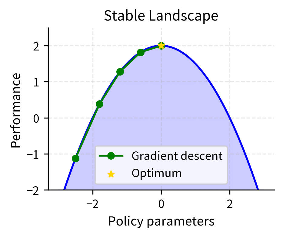
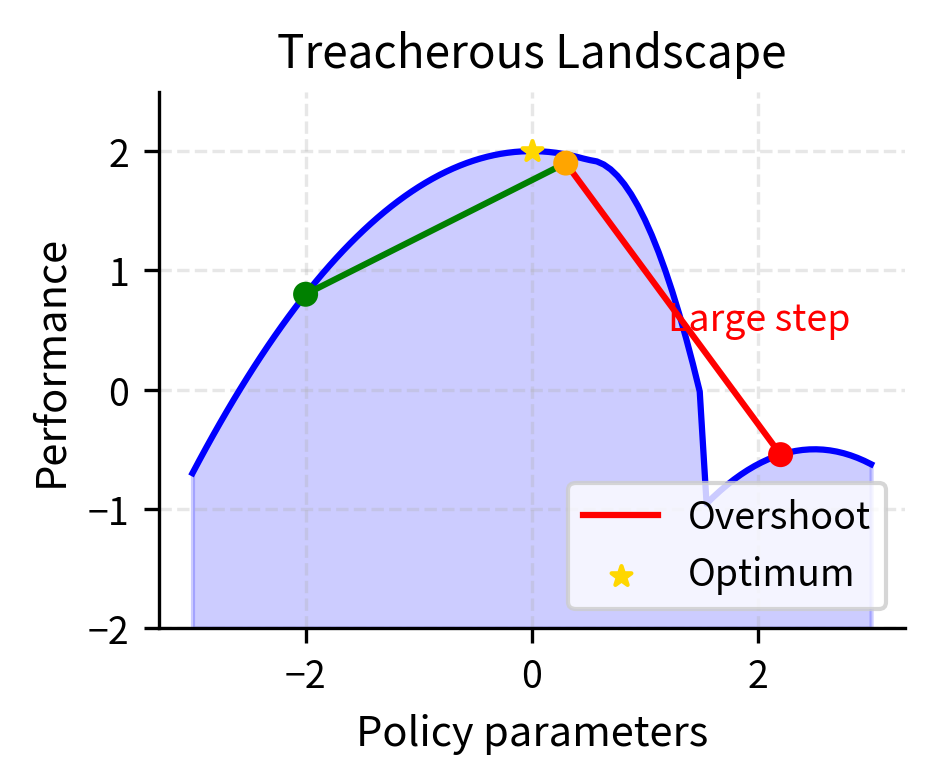
The fundamental issue with this formulation is that the gradient provides no guidance about step size. The policy gradient theorem tells us which direction to move parameters to increase expected reward, but it remains entirely silent about how far we should move in that direction. This is analogous to knowing that walking north takes you closer to your destination but not knowing whether to take one step or one hundred steps. A step in the gradient direction improves performance locally, within an infinitesimally small neighborhood around the current parameters. However, nothing in the mathematics prevents taking such a large step that you overshoot into a region where the policy performs terribly. The landscape of policy performance is not smooth—it contains cliffs, plateaus, and treacherous regions where a policy that seemed promising suddenly fails catastrophically.

This problem is especially acute because of three interconnected challenges:

• Non-stationary data distribution: The policy generates its own training data. When the policy changes significantly, the state distribution also changes, potentially invalidating previously learned value estimates.
• High variance: Policy gradient estimates are inherently noisy, making it difficult to distinguish signal from noise.
• Irreversibility: A bad update might move the policy to a region where it never encounters states that would help it recover.

Consider a language model learning from human feedback. If a single gradient update makes the model much more likely to generate certain patterns, the model might suddenly produce outputs that are completely off-distribution from its training, leading to reward model extrapolation errors and further degradation.

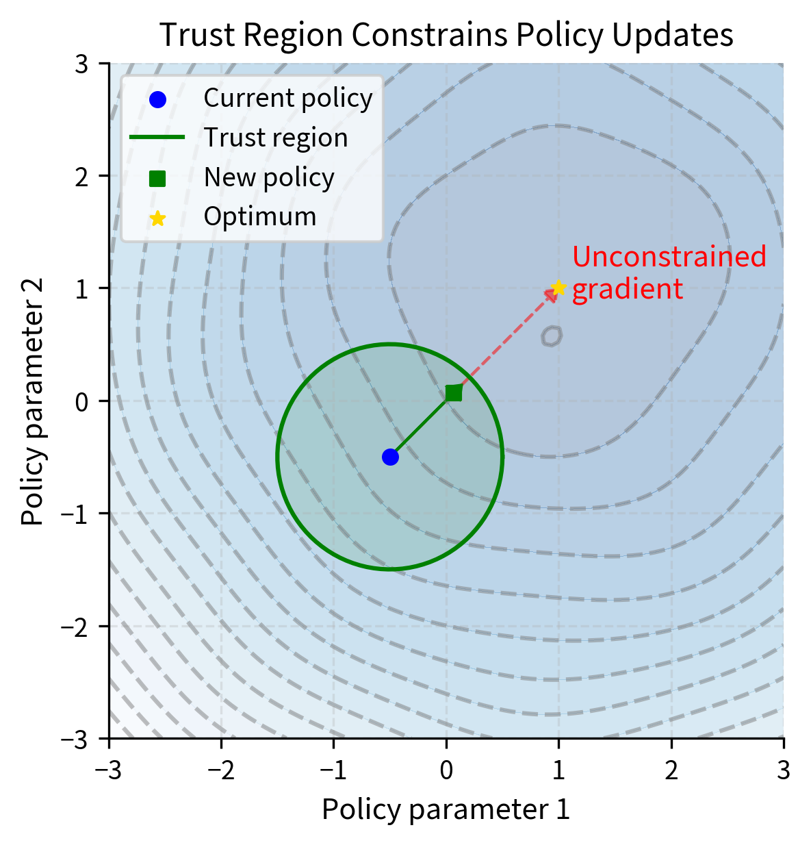
The insight behind trust region methods is to constrain how much the policy can change in each update. Rather than blindly following the gradient wherever it leads, we optimize the policy subject to a constraint. This constraint keeps the new policy "close" to the old one. This approach recognizes a fundamental tension in optimization: we want to improve the policy as quickly as possible. However, our confidence in the improvement direction decreases the further we move from where we collected our data.

A trust region formalizes an important limitation. Our confidence in gradient-based improvements decreases as we move away from where we collected data. Gradients computed from sampled trajectories indicate how to improve performance near observed states and actions. Moving far from the current policy means extrapolating beyond our data rather than interpolating, making gradient estimates less reliable. The trust region formalizes the boundary beyond which you should not venture without collecting new data.

Trust Region Policy Optimization (TRPO), PPO's predecessor, formalizes this using KL divergence as a constraint. The KL divergence measures how different two probability distributions are, making it a natural choice for measuring policy similarity. Policies that assign similar probabilities to actions have low KL divergence, while policies that behave very differently have high KL divergence.

The TRPO objective addresses the policy update problem by maximizing expected advantage while explicitly constraining how much the policy can change. It maximizes the expected advantage weighted by the importance sampling ratio, which allows us to use data from the old policy to evaluate the new policy, while constraining the KL divergence between old and new policies:

To understand how this constrained optimization problem balances improvement against stability, examine each component:

• $\theta$: parameters of the new policy being optimized
• $\theta_{\text{old}}$: parameters of the old policy from which data was collected
• $\mathbb{E}_{s, a \sim \pi_{\theta_{\text{old}}}}$: expectation over states and actions sampled from trajectories collected using the old policy
• $s$: a state sampled from the state distribution under the old policy
• $a$: an action sampled from the old policy in state $s$
• $\pi_\theta(a|s)$: probability of action $a$ in state $s$ under the new policy
• $\pi_{\theta_{\text{old}}}(a|s)$: probability of action $a$ in state $s$ under the old policy
• $\frac{\pi_\theta(a|s)}{\pi_{\theta_{\text{old}}}(a|s)}$: the importance sampling ratio, which reweights data from the old policy to evaluate the new policy
• $A^{\pi_{\theta_{\text{old}}}}(s, a)$: advantage function computed under the old policy, measuring how much better action $a$ is than average in state $s$
• $\mathbb{E}_s$: expectation over states from the state distribution under the old policy
• $D_{\text{KL}}(\pi_{\theta_{\text{old}}} \| \pi_\theta)$: Kullback-Leibler divergence measuring how much the new policy distribution differs from the old policy distribution
• $\delta$: maximum allowed KL divergence, the trust region radius

This constraint ensures the new policy $\pi_\theta$ doesn't diverge too far from the old policy $\pi_{\theta_{\text{old}}}$ in terms of the probability distributions over actions. The ratio $\frac{\pi_\theta(a|s)}{\pi_{\theta_{\text{old}}}(a|s)}$ is called the importance sampling ratio and allows us to evaluate the new policy using data collected from the old policy. This ratio acts as a correction factor: if the new policy is twice as likely to take an action as the old policy, we weight that action's contribution twice as heavily to account for the fact that it would occur more frequently under the new policy.

TRPO guarantees monotonic improvement under certain conditions, meaning the policy never gets worse than the previous version. This guarantee provides the stability that vanilla policy gradients lack. However, the mathematical machinery required to enforce this guarantee comes with significant computational costs: computing Fisher information matrices and solving linear systems.

Solving the constrained optimization problem requires computing second-order derivatives, specifically the Fisher information matrix, and performing conjugate gradient optimization to solve a system of linear equations. This makes TRPO computationally expensive and difficult to implement correctly. Computing the Fisher information matrix across multiple workers in distributed settings adds significant overhead.

PPO achieves similar stability guarantees with a first-order method by replacing the hard constraint with a penalty built directly into the objective function. Instead of solving a constrained optimization problem, PPO modifies the objective itself to discourage excessive policy changes. This transformation from constraint to penalty makes PPO dramatically simpler to implement while preserving the essential benefits of trust region methods.

The probability ratio is central to PPO. It quantifies how much the new policy's probability for an action differs from the old policy's probability. By examining this ratio across all observed state-action pairs, you can assess whether the policy is changing appropriately or excessively. Define:

Understanding what each symbol represents helps illuminate why this ratio captures policy change so effectively:

• $r_t(\theta)$: the importance sampling ratio at timestep $t$
• $\pi_\theta(a_t|s_t)$: probability of action $a_t$ in state $s_t$ under the new policy with parameters $\theta$
• $\pi_{\theta_{\text{old}}}(a_t|s_t)$: probability of the same action in the same state under the old policy
• $a_t$: the action taken at timestep $t$
• $s_t$: the state at timestep $t$
• $\theta$: parameters of the new policy
• $\theta_{\text{old}}$: parameters of the old policy

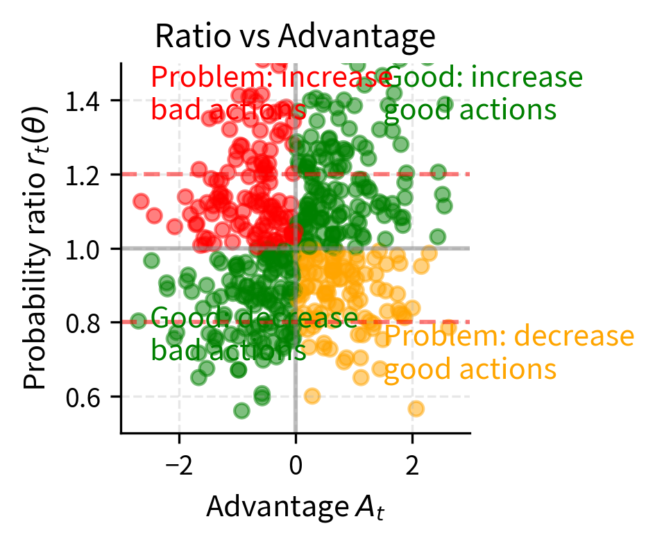
This ratio captures how much more or less likely action $a_t$ becomes under the new policy compared to the old one. The interpretation is intuitive and direct:

• $r_t(\theta) = 1$: the new policy assigns the same probability to this action; no change from the old policy
• $r_t(\theta) > 1$: the new policy makes this action more likely (for example, $r_t = 2$ means the new policy is twice as likely to take this action)
• $r_t(\theta) < 1$: the new policy makes this action less likely (for example, $r_t = 0.5$ means the new policy is half as likely to take this action)

This ratio directly measures behavioral change. A ratio of 1 everywhere indicates identical policies, while very large or very small ratios indicate dramatic behavioral shifts. This makes the ratio ideal for clipping to constrain policy changes.

The standard policy gradient objective can be rewritten using this ratio, revealing its fundamental role in policy optimization:

To understand how the ratio enables policy improvement, examine what each term contributes:

• $L^{\text{PG}}(\theta)$: the policy gradient objective function we want to maximize
• $\mathbb{E}_t$: expectation over timesteps in collected trajectories
• $r_t(\theta)$: the probability ratio at timestep $t$, equal to $\frac{\pi_\theta(a_t|s_t)}{\pi_{\theta_{\text{old}}}(a_t|s_t)}$
• $A_t$: the advantage estimate at timestep $t$, measuring how much better the action taken was compared to the average action
• $\theta$: parameters of the policy being optimized

When $\theta = \theta_{\text{old}}$, we have $r_t(\theta) = 1$ everywhere, and the objective reduces to the simple advantage-weighted sum. The gradient of this objective at $\theta = \theta_{\text{old}}$ equals the standard policy gradient, confirming that this formulation is equivalent to what we derived earlier.

The problem becomes clear when we consider what happens as we optimize this objective. As the optimizer works to maximize the expected reward, the ratio can become arbitrarily large or small. If an action had positive advantage, indicating it was better than expected, unconstrained optimization would keep increasing its probability without bound. The gradient always points toward making good actions more likely and bad actions less likely, but nothing in this formulation limits how far the policy can shift. This is precisely the instability problem that TRPO addressed with its KL constraint, and that PPO addresses with clipping.

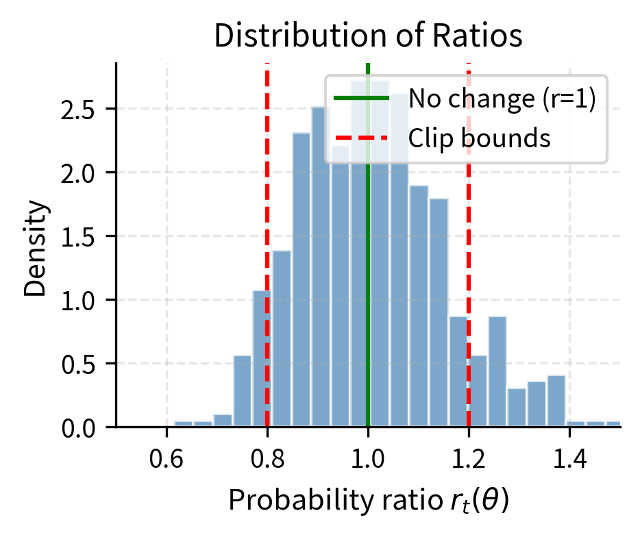
PPO's key innovation is straightforward: clip the probability ratio to remove incentives for excessive policy changes. Rather than imposing a hard constraint requiring complex optimization machinery, PPO modifies the objective function itself, so large policy changes provide no additional benefit. The clipped surrogate objective is:

where $\epsilon$ is a hyperparameter, typically set between 0.1 and 0.2, that defines the trust region width. This single parameter controls how much the policy can change in each update.

To understand precisely how clipping constrains the ratio, you need to examine the clip function itself. The clip function constrains the probability ratio to remain within the interval $[1-\epsilon, 1+\epsilon]$, defined as:

Each component of this piecewise function serves a specific purpose:

• $r$: the input value to be clipped; in PPO, this is $r_t(\theta)$, the probability ratio
• $1-\epsilon$: the lower bound of the allowed range
• $1+\epsilon$: the upper bound of the allowed range
• The function returns $r$ unchanged if it's within the bounds, otherwise returns the nearest bound

The key intuition is that this clipping removes the gradient signal when the ratio moves outside the trust region. Consider what happens during optimization: you want the optimizer to adjust parameters to increase the objective. If the new policy is already making an action much more likely, with a ratio greater than $1+\epsilon$, or much less likely, with a ratio less than $1-\epsilon$, than the old policy, clipping prevents the optimizer from pushing it even further in that direction. The clipped term becomes constant with respect to the parameters, meaning its gradient is zero, so there is no signal encouraging further movement in that direction.

This clipped ratio is then used in computing the clipped surrogate objective. Returning to the full $L^{\text{CLIP}}(\theta)$ formula and examining it in detail:

Each component plays a specific role in creating stable policy updates:

• $L^{\text{CLIP}}(\theta)$: the clipped surrogate objective that PPO maximizes
• $\mathbb{E}_t$: expectation over all timesteps in the collected batch
• $\min(\cdot, \cdot)$: takes the smaller of the two arguments (the pessimistic bound)
• $r_t(\theta)$: the probability ratio $\frac{\pi_\theta(a_t|s_t)}{\pi_{\theta_{\text{old}}}(a_t|s_t)}$
• $A_t$: the advantage estimate at timestep $t$
• $\epsilon$: the clipping parameter, typically 0.1 to 0.2, that defines the trust region
• $\text{clip}(r_t(\theta), 1-\epsilon, 1+\epsilon)$: constrains the ratio to the interval $[1-\epsilon, 1+\epsilon]$

The $\min$ operation is crucial. It selects the smaller of the unclipped and clipped objectives, ensuring a pessimistic (conservative) bound on the improvement. By always choosing the lower value, we prevent the optimizer from being overly optimistic about improvements that would require large policy changes. We'll analyze both cases based on the sign of the advantage:

Case 1: Positive Advantage ($A_t > 0$)

When an action is better than expected (positive advantage), we want to increase its probability. The unclipped objective's gradient pushes the policy to make this action more likely, but PPO limits the extent.

• If $r_t(\theta) > 1 + \epsilon$: The clipped term $(1+\epsilon) A_t$ is smaller than $r_t(\theta) A_t$, since $A_t > 0$ and $1+\epsilon < r_t(\theta)$. The $\min$ selects the clipped term $(1+\epsilon) A_t$, which is constant with respect to $\theta$, so the gradient is zero and provides no incentive for us to increase the ratio further.
• If $r_t(\theta) \leq 1 + \epsilon$: Both terms are equal or the unclipped term is smaller, so normal optimization proceeds.

This means that once the probability ratio exceeds $1+\epsilon$, the optimizer receives no additional reward for increasing it further. The policy has already been sufficiently encouraged to take this good action.

Case 2: Negative Advantage ($A_t < 0$)

When an action is worse than expected (negative advantage), we want to decrease its probability. The unclipped objective's gradient encourages this, but PPO limits the extent:

• If $r_t(\theta) < 1 - \epsilon$: Since $A_t < 0$, multiplying by smaller values makes the product more negative. The clipped term $(1-\epsilon) A_t$ is larger (less negative) than the unclipped term $r_t(\theta) A_t$ because $r_t(\theta) < 1-\epsilon$. The $\min$ selects the more negative unclipped term. Since the clipped term $(1-\epsilon) A_t$ is constant, its gradient is zero and the objective becomes flat once $r_t(\theta)$ drops below $1-\epsilon$, preventing the policy from decreasing the probability further.
• If $r_t(\theta) \geq 1 - \epsilon$: Normal optimization proceeds.

This prevents the policy from becoming too averse to actions that happened to have negative advantage. Such actions might still be valuable in other states, and excessively penalizing them could harm overall performance.

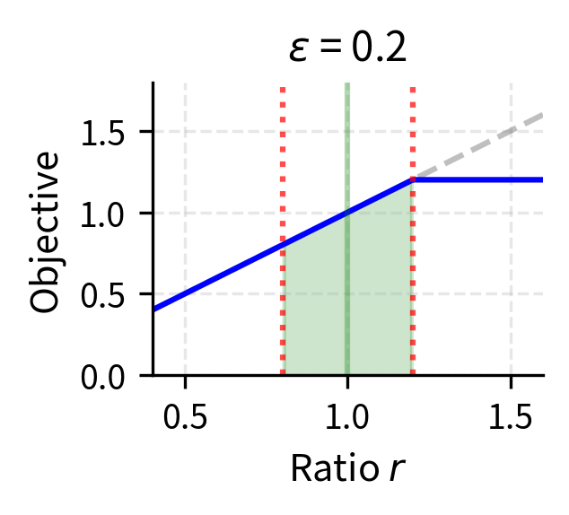
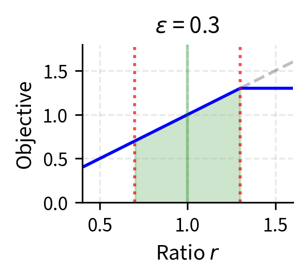
The following figure illustrates this behavior:

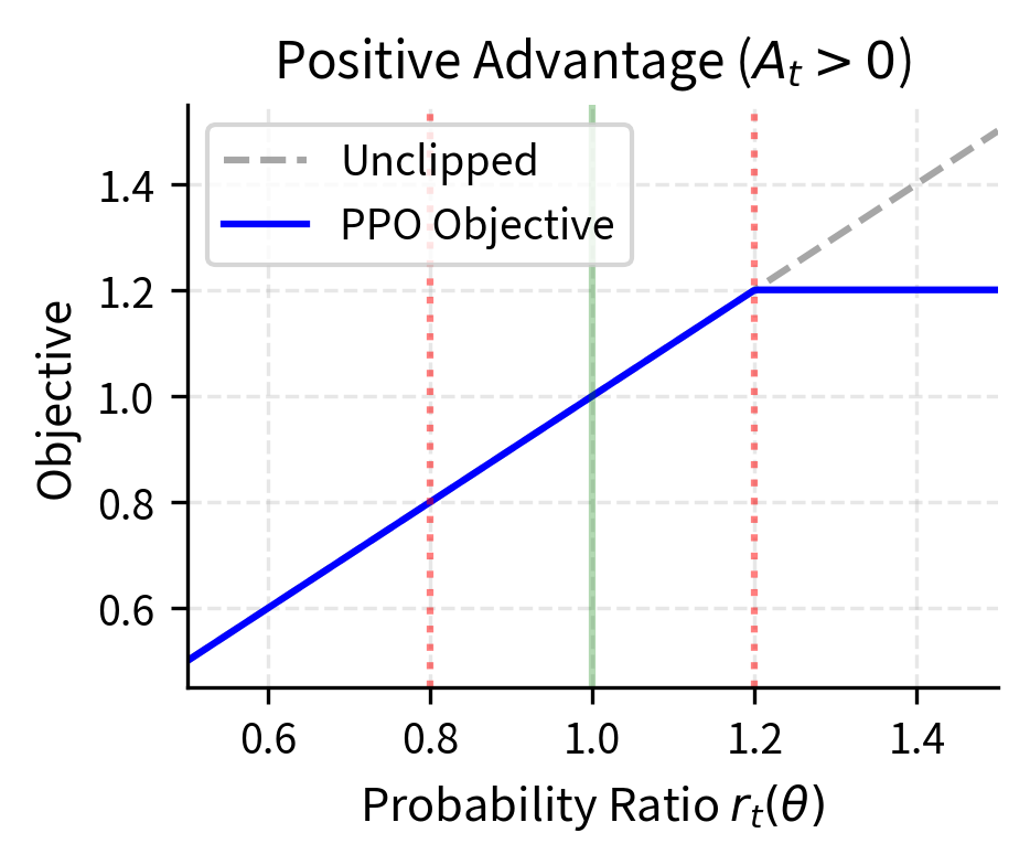
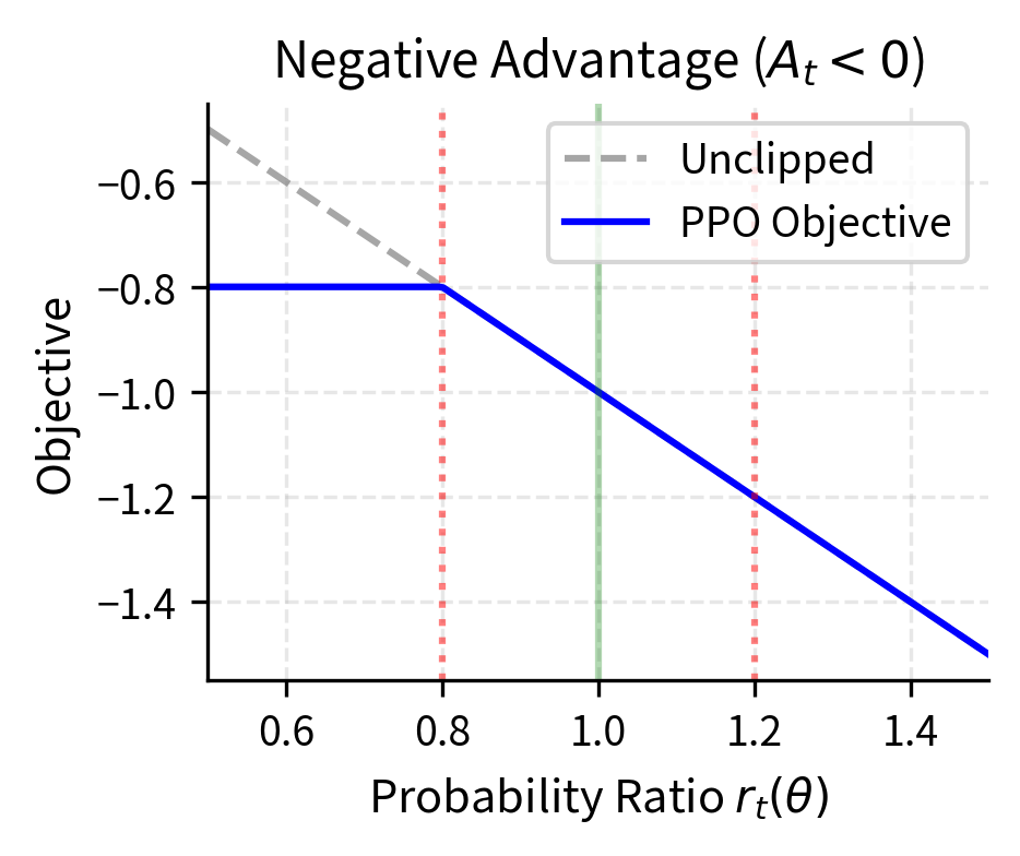
The key insight from examining these plots is that clipping creates a "pessimistic bound" on the objective. When the policy tries to change too much, the objective flattens and provides no gradient signal to continue. This self-limiting behavior makes PPO stable without requiring the complex second-order optimization of TRPO.

PPO typically uses Generalized Advantage Estimation (GAE) to compute advantages with a controllable bias-variance tradeoff. The advantage function measures how much better an action is than average. True advantages depend on full trajectory information unavailable during learning, so you must estimate them from observed rewards. Different estimation approaches trade off bias against variance in different ways.

A one-step estimate uses only the immediate reward and next state value, providing low variance, since it depends on fewer random variables, but high bias, since it relies heavily on the accuracy of the value function. A Monte Carlo estimate uses all future rewards until episode end, providing low bias, since it uses actual observed returns, but high variance, since it incorporates the randomness of many future actions and transitions.

GAE solves this estimation problem by taking an exponentially weighted average of temporal difference errors at different time horizons. The parameter $\lambda$ controls how quickly the weights decay as we look further into the future. This approach combines the benefits of using both short-term (low variance but high bias) and long-term (high variance but low bias) estimates. By tuning $\lambda$, we can find the sweet spot for our particular problem.

GAE is defined as:

Each component of this formula contributes to the bias-variance tradeoff:

• $\hat{A}_t^{\text{GAE}(\gamma, \lambda)}$: the GAE advantage estimate at timestep $t$
• $\sum_{l=0}^{\infty}$: sum over all future timesteps from the current timestep forward (in practice, truncated at episode end)
• $l$: the lookahead index, indicating how many steps into the future we're considering
• $\gamma$: the discount factor, typically 0.99, which determines how much we value future rewards
• $\lambda$: the GAE parameter, typically 0.95, which controls the bias-variance tradeoff
• $(\gamma \lambda)^l$: the exponentially decaying weight for the $l$-step temporal difference error
• $\delta_{t+l}$: the temporal difference (TD) error at timestep $t+l$
• $t$: the current timestep

The temporal difference error, which serves as the building block for GAE, measures the discrepancy between what we expected and what we observed, and is defined as:

Understanding each term clarifies why TD errors are useful for advantage estimation:

• $\delta_t$: the temporal difference error at timestep $t$, measuring the difference between the observed reward plus next state value versus the current state value
• $r_t$: the immediate reward received at timestep $t$
• $\gamma$: the discount factor
• $V(s_t)$: the value function estimate for state $s_t$ (the predicted cumulative future reward)
• $V(s_{t+1})$: the value function estimate for the next state
• $\gamma V(s_{t+1})$: the discounted value of the next state
• $s_t$: the state at timestep $t$
• $s_{t+1}$: the next state at timestep $t+1$

The TD error intuition is clear: if our value function were perfect, the expected TD error would be zero. The value of the current state should equal the immediate reward plus the discounted value of the next state. A positive TD error indicates we received more reward than expected, suggesting the action was good. A negative TD error indicates we received less than expected.

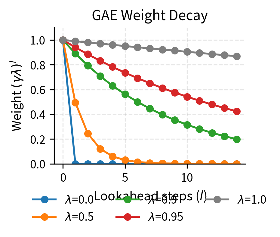
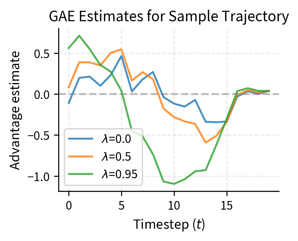
The tradeoff controlled by $\lambda$ determines how we combine information across time horizons:

• $\lambda = 0$ uses only one-step TD error (low variance, high bias)
• $\lambda = 1$ uses full Monte Carlo returns (high variance, low bias)

In practice, $\lambda = 0.95$ provides a good balance for most problems, weighting nearby TD errors heavily while still incorporating longer-term information with diminishing weight.

The recursive formulation for efficient computation eliminates the need to store and sum all future TD errors explicitly:

Each component of this recursive formula has a clear interpretation:

• $\hat{A}_t$: the advantage estimate at timestep $t$, computed recursively
• $\delta_t$: the temporal difference error at timestep $t$, equal to $r_t + \gamma V(s_{t+1}) - V(s_t)$
• $\gamma$: discount factor
• $\lambda$: GAE parameter
• $\hat{A}_{t+1}$: the advantage estimate for the next timestep, computed first in backward iteration
• $t$: the current timestep

The boundary condition is $\hat{A}_T = 0$ at the terminal timestep, since there are no future advantages after the episode ends. This recursive formulation is computationally efficient because we can compute all advantages in a single backward pass through the trajectory, starting from the end and working toward the beginning. Each computation reuses the result from the next timestep, avoiding redundant calculations.

The full PPO objective combines three terms: policy improvement, value function training, and exploration. These components work together synergistically. Accurate value estimates enable meaningful advantages, while exploration discovers strategies that improve both the policy and value function. The complete objective is:

Each component serves a distinct purpose in training a capable agent:

• $L^{\text{PPO}}(\theta)$: the complete PPO objective function, to be maximized
• $\mathbb{E}_t$: expectation over timesteps in the batch
• $L^{\text{CLIP}}(\theta)$: the clipped surrogate objective for policy improvement, defined earlier
• $c_1$: coefficient for the value function loss, typically 0.5
• $L^{\text{VF}}(\theta)$: the value function loss, which encourages accurate value estimates
• $c_2$: coefficient for the entropy bonus, typically 0.01
• $S[\pi_\theta](s_t)$: the entropy of the policy distribution at state $s_t$, which encourages exploration
• $\theta$: parameters of both the policy and value networks, when they share parameters
• $s_t$: the state at timestep $t$

The value function loss has a negative sign because we minimize loss while maximizing the overall objective. This sign convention means that minimizing value function error increases the overall objective, aligning all components toward the same optimization direction.

The three terms work together synergistically. The clipped surrogate loss $L^{\text{CLIP}}$ improves the policy by increasing probabilities of high-advantage actions while respecting the trust region constraint. The value function loss $L^{\text{VF}}$ trains the value function to make accurate predictions. These predictions are essential for computing meaningful advantages in future updates. The entropy term $S$ encourages exploration by penalizing overly deterministic policies. This prevents premature convergence and helps the agent discover better strategies.

The value function $V_\phi(s)$ predicts expected cumulative returns and is trained alongside the policy. Accurate value estimates are essential because the value function serves as the baseline in advantage computation. Without accuracy, advantages become noisy and unreliable, leading to high-variance policy gradients that destabilize training.

The value function predicts expected cumulative future rewards starting from each state under the current policy. You train the value function by minimizing the mean squared error between its predictions and target values, computed as:

Understanding each component reveals the standard regression structure of value function training:

• $L^{\text{VF}}(\phi)$: the value function loss, the mean squared error
• $\mathbb{E}_t$: expectation over timesteps in the batch
• $\phi$: parameters of the value function network
• $V_\phi(s_t)$: the value function's prediction for state $s_t$ under current parameters
• $V_t^{\text{target}}$: the target value we want the value function to predict
• $s_t$: the state at timestep $t$
• $(V_\phi(s_t) - V_t^{\text{target}})^2$: the squared difference between prediction and target

The target value is computed as:

Each term in this target construction serves a specific purpose:

• $V_t^{\text{target}}$: the target value for the value function to predict at timestep $t$
• $\hat{A}_t$: the advantage estimate at timestep $t$, computed using GAE
• $V_{\phi_{\text{old}}}(s_t)$: the value prediction from the old value function, before this update
• $\phi_{\text{old}}$: parameters of the value function from the previous update
• $s_t$: the state at timestep $t$

This target construction guides the value function to predict returns accurately using computed advantages. The advantage $\hat{A}_t$ represents how much better actual returns were than expected, or equivalently, the residual between actual returns and predicted returns. Adding this residual to the old value estimate $V_{\phi_{\text{old}}}(s_t)$ yields an improved return estimate.

This bootstrapping approach allows the value function to learn from its own predictions while incorporating new information from observed rewards. The process is iterative. Better value estimates lead to better advantage estimates, which lead to better policy updates, which generate better training data for the value function. Some implementations also clip the value function loss similarly to the policy loss, preventing large changes to the value function that might destabilize this iterative process.

Entropy measures randomness in the policy's action distribution. High entropy spreads probability across multiple actions instead of concentrating on one choice. Encouraging higher entropy prevents the policy from becoming deterministic too early, which keeps exploration alive and enables discovery of better strategies.

For a policy distribution at state $s_t$, entropy is defined as:

Each component of this formula connects to information-theoretic concepts:

• $S[\pi_\theta](s_t)$: the entropy of the policy distribution at state $s_t$
• $\sum_a$: sum over all possible actions in the action space
• $a$: an action from the action space
• $\pi_\theta(a|s_t)$: the probability of action $a$ in state $s_t$ under the current policy
• $\log \pi_\theta(a|s_t)$: the log probability of action $a$
• $\theta$: parameters of the policy network
• $s_t$: the state at timestep $t$

This entropy term encourages exploration by rewarding policies that maintain uncertainty over actions. The formula measures the expected information content, or surprise, in the policy's action distribution. Mathematically, when action probabilities are uniform, meaning all actions are equally likely, the sum of $\pi_\theta(a|s_t) \log \pi_\theta(a|s_t)$ terms is maximized in magnitude, giving high entropy.

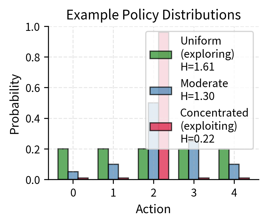
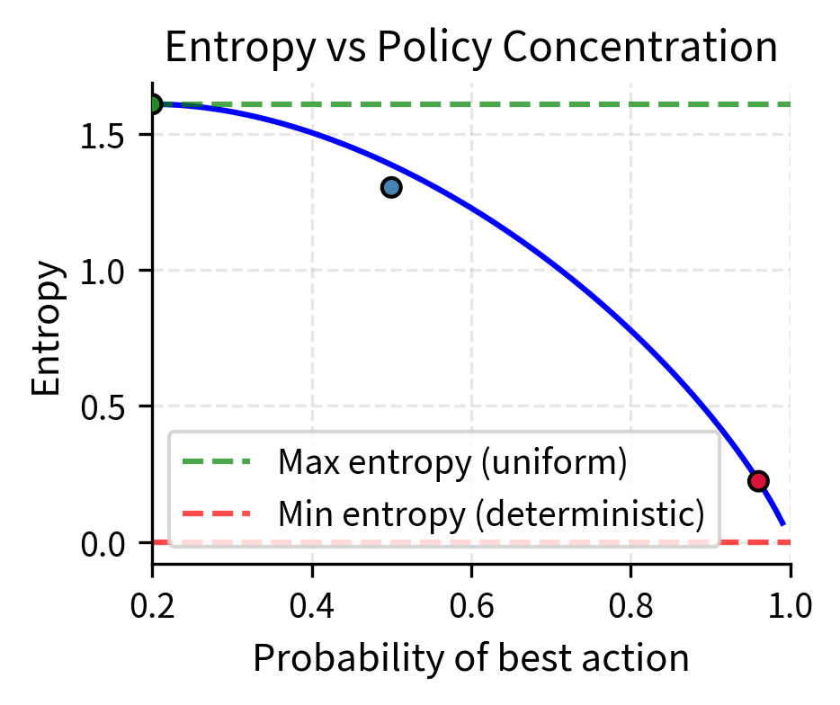
When all actions have similar probabilities, indicating high uncertainty, entropy is maximized. This reflects the fact that an observer would be maximally uncertain about which action the policy will choose. When the policy becomes deterministic, meaning one action has probability near 1 and all others near 0, entropy approaches zero. The policy reveals little information because its behavior is predictable. While deterministic policies can be desirable in final deployment, during training we need exploration to discover better strategies.

The coefficient $c_2$ (typically 0.01) controls the exploration-exploitation tradeoff. Higher values encourage exploration but may slow convergence to optimal behavior. Lower values enable faster convergence but risk getting stuck in suboptimal local minima.

The typical coefficient values are:

• $c_1 = 0.5$: weight for value function loss
• $c_2 = 0.01$: weight for entropy bonus
• $\epsilon = 0.2$: clipping parameter

Sharing parameters between policy and value networks, which is common in practice, combines all three losses for joint optimization. This parameter sharing encourages the network to learn representations useful for both predicting values and selecting actions. It often improves sample efficiency compared to separate networks.

We'll implement PPO for continuous control using a simple environment. This lets you focus on the algorithm rather than domain-specific complexity.

You'll implement an actor-critic architecture where the policy (actor) and value function (critic) share some layers:

This architecture implements the actor-critic pattern for continuous control. The shared feature extractor (two 64-unit hidden layers) learns representations useful for both policy and value prediction. The actor head outputs Gaussian parameters (mean and learnable log standard deviation), enabling sampling of continuous actions with exploration noise. The critic head predicts state values for advantage computation. The get_action method samples actions during rollout collection. The evaluate_actions method computes log probabilities and entropy during policy updates.

We collect experience in rollout buffers and compute advantages before each update:

The RolloutBuffer manages experience collection and advantage computation. The add method stores each transition (state, action, reward, value estimate, log probability, done flag) during rollout. The compute_returns_and_advantages method implements GAE by iterating backwards through the trajectory, computing temporal difference errors and accumulating them with exponential decay controlled by gamma and lambda. This backward pass efficiently computes advantages for all timesteps in a single sweep. The get_batches method shuffles the data and yields minibatches for multiple optimization epochs, improving sample efficiency.

The core PPO update computes the clipped objective and performs multiple epochs of minibatch updates:

Notice several important details:

• Advantage normalization (zero mean, unit variance) stabilizes training
• Probability ratios are computed in log space for numerical stability: $r = \exp(\log \pi_{\theta}(a|s) - \log \pi_{\theta_{\text{old}}}(a|s))$ (avoids underflow)
• Gradient clipping prevents exploding gradients
• Gradient clipping prevents exploding gradients
• Multiple epochs of updates reuse collected data, improving sample efficiency

Now let's put everything together in a training loop:

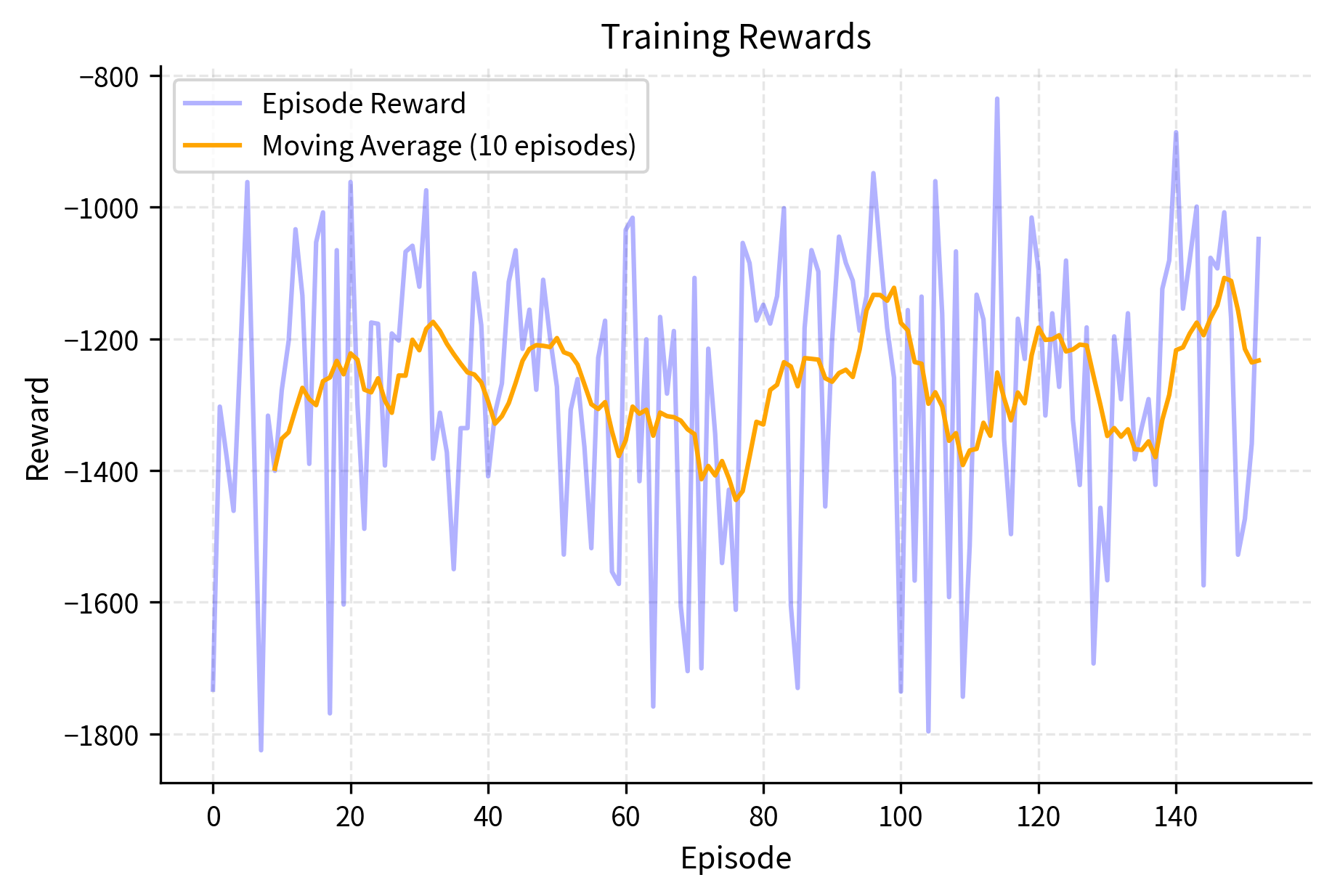
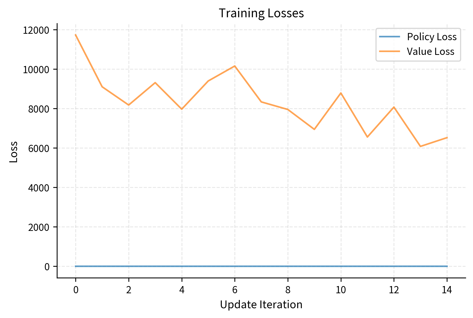
The training loop orchestrates PPO by repeating the following cycle: collect rollouts from executing the current policy, compute advantages using GAE with bootstrapped final values, perform multiple minibatch update epochs with the clipped objective, and track metrics. The loop continues until reaching the total timestep budget. Episodes can terminate from either environment termination or truncation.

The training results demonstrate successful learning. The total episode count shows how many complete episodes occurred during the 30,000 timestep budget. The final average reward, computed over the last 10 episodes, indicates current policy performance, while the best average reward shows peak performance achieved during training. These metrics confirm PPO successfully learned to balance the pendulum, with steady performance improvement as the algorithm optimized both policy and value networks.

We can visualize the training progress by plotting episode rewards and losses over time:

PPO's performance depends on several key hyperparameters:

• Clip parameter ($\epsilon$): Controls policy change by defining the trust region as $[1-\epsilon, 1+\epsilon]$ for the probability ratio. Values of 0.1 to 0.3 are typical. Smaller values (e.g., 0.05) constrain updates too tightly and slow learning. Larger values (e.g., 0.5) provide insufficient constraint and risk instability.
• GAE lambda ($\lambda$): Bias-variance tradeoff for advantage estimation. Values of 0.95 to 0.99 are typical.
• Number of epochs: Number of passes through collected data. Using 3 to 10 epochs balances sample efficiency against overfitting to old data.
• Minibatch size: Larger batches provide more stable gradients but may overfit. Sizes of 32 to 256 are common.
• Rollout length: How much data to collect before updating. Longer rollouts provide better advantage estimates but slower iteration.
• Learning rate: Values of 1e-4 to 3e-4 are typical for PPO. You can use learning rate scheduling to improve convergence.

Language model implementations often require adjusted values. The next chapter explores LLM-specific considerations.

The key parameters for PPO are:

• clip_epsilon: The clipping parameter that defines the trust region width (typically 0.1 to 0.3). Smaller values provide tighter constraints on policy updates, while larger values allow more aggressive changes.
• gae_lambda: Controls bias-variance tradeoff in advantage estimation (typically 0.95 to 0.99). Higher values use longer horizons for advantage computation.
• n_epochs: Number of optimization epochs per rollout (typically 3 to 10). More epochs extract more learning from each batch but risk overfitting to old data.
• batch_size: Minibatch size for gradient updates (typically 32 to 256). Larger batches provide more stable gradients.
• rollout_length: Number of timesteps to collect before updating (typically 2048 for simple tasks). Longer rollouts provide better advantage estimates.
• value_coef: Coefficient for value function loss in total objective (typically 0.5). Controls how much weight to give value function training relative to policy training.
• entropy_coef: Coefficient for entropy bonus (typically 0.01). Higher values encourage more exploration.

PPO revolutionized practical reinforcement learning and became the foundation for aligning large language models. Its impact comes from achieving trust region stability without the computational complexity of TRPO. Before PPO, reliable RL training required extensive expertise and environment-specific tuning. PPO made RL accessible to new domains.

PPO has important limitations. The clipping mechanism provides only approximate trust region enforcement, so the policy can still drift significantly over many updates, especially with high learning rates or many epochs. This drift becomes problematic in RLHF settings where maintaining proximity to the supervised fine-tuned base model is essential for response quality.

Sample efficiency is a concern. PPO requires substantial environment or reward model interaction to learn effectively. Data becomes stale after a few update epochs, requiring fresh collection. For language models, reward model queries are expensive, motivating direct alignment methods like DPO.

PPO inherits challenges from actor-critic methods. The value function must accurately estimate expected returns for meaningful advantages. In high-dimensional state spaces like language, value estimation becomes noisy, producing high-variance gradients despite advantage normalization.

PPO also optimizes for the provided reward signal without accounting for reward model uncertainty. This can lead to reward hacking, where the policy exploits reward model quirks rather than genuinely improving. The next chapter discusses how KL divergence penalties and reference model constraints mitigate this problem in RLHF.

PPO addresses vanilla policy gradient instability through a clipped surrogate objective that constrains policy changes in each update. Key insights include:

• Trust regions matter: Constraining policy updates prevents severe performance degradation.
• Clipping approximates constraints: Rather than solving a constrained optimization problem, PPO clips the objective to remove incentives for excessive changes.
• Pessimistic bounds ensure stability: The min operation between clipped and unclipped objectives prevents overestimating improvement.
• Multiple epochs improve efficiency: Multiple epochs of updates reuse collected data, improving sample efficiency.

The full PPO objective combines the clipped policy loss with a value function loss for training the critic and an entropy bonus for exploration. Generalized Advantage Estimation provides a controllable bias-variance tradeoff for computing advantages.

PPO's stability, simplicity, and sample efficiency made it the standard algorithm for RLHF in language models. The next chapter explores adapting PPO for language model alignment by covering reference model constraints and generation-specific considerations.

Ready to test your understanding? Take this quick quiz to reinforce what you've learned about Proximal Policy Optimization.