PPO for Language Models: Adapting RL to Text Generation

In the previous chapter, we explored the PPO algorithm as a general-purpose policy gradient method with clipped objectives and value function estimation. Now we face a crucial question: how do we apply these ideas to language models? The translation is difficult because traditional reinforcement learning and text generation have fundamental differences. Language models were designed as next-token predictors, not as agents acting in environments. They were trained to model the statistical patterns of human language, not to maximize cumulative rewards over time. Yet with some careful reframing, we can view text generation through the lens of sequential decision-making and apply PPO to steer models toward human-preferred outputs.

This chapter connects reinforcement learning to the structure of language generation. We will see how an LLM naturally serves as a stochastic policy, why the vocabulary forms a massive discrete action space, and how rewards propagate through generated sequences. Most importantly, we will understand why constraining the policy to stay close to its original behavior is essential for stable training. Each of these concepts builds on the last, forming a complete picture of how PPO transforms language model behavior.

In reinforcement learning, a policy maps states to action probabilities. Given a state $s$, the policy $\pi(a|s)$ tells us the probability of taking action $a$. This definition describes decision-making: the agent observes its state, checks its policy, and chooses an action. Language models do the same: given a context, the model outputs a probability distribution over the next token. The parallel is exact.

To see this clearly, consider what happens when you type a prompt. The model processes your input, builds internal representations through its transformer layers, and produces a probability distribution over its vocabulary. This distribution assigns higher probabilities to tokens that would naturally continue the text and lower probabilities to tokens that would seem out of place. When the model generates a response, it samples from this distribution (or selects greedily), appends the chosen token to the context, and repeats the process. Each step involves observing a state and selecting an action according to a probability distribution, which is exactly what a policy does.

Let $x = (x_1, x_2, \ldots, x_n)$ denote the input prompt and $y = (y_1, y_2, \ldots, y_T)$ the generated response. At each generation step $t$, the language model computes:

where:

• $\pi_\theta$: the policy defined by model parameters $\theta$
• $y_t$: the token generated at the current step $t$
• $x$: the input prompt sequence
• $y_{<t}$: the sequence of tokens generated prior to step $t$, $(y_1, \ldots, y_{t-1})$

This represents the probability of generating token $y_t$ given the full context of the prompt and previous tokens. The notation emphasizes that the policy depends on everything that came before: the original prompt establishes the task, and each previously generated token shapes what should come next. The model's parameters $\theta$ encode the learned patterns that determine how context maps to token probabilities.

Comparing language models to standard RL shows:

• State $s_t$: The concatenation of the prompt and all tokens generated so far, $(x, y_1, \ldots, y_{t-1})$
• Action $a_t$: The next token to generate, $y_t$
• Policy $\pi_\theta(a_t|s_t)$: The LLM's softmax output distribution over the vocabulary
• Trajectory $\tau$: The complete prompt-response pair $(x, y)$

The autoregressive generation process that produces a response is exactly a policy rollout. Starting from the initial state $s_1 = x$, we sample actions according to the policy, each action extends the state, and we continue until generating a stop token. This equivalence is not just a useful metaphor; it is a precise mathematical correspondence that allows us to apply policy gradient methods to language generation. Policy optimization theorems and techniques apply to steering language models toward desired behaviors.

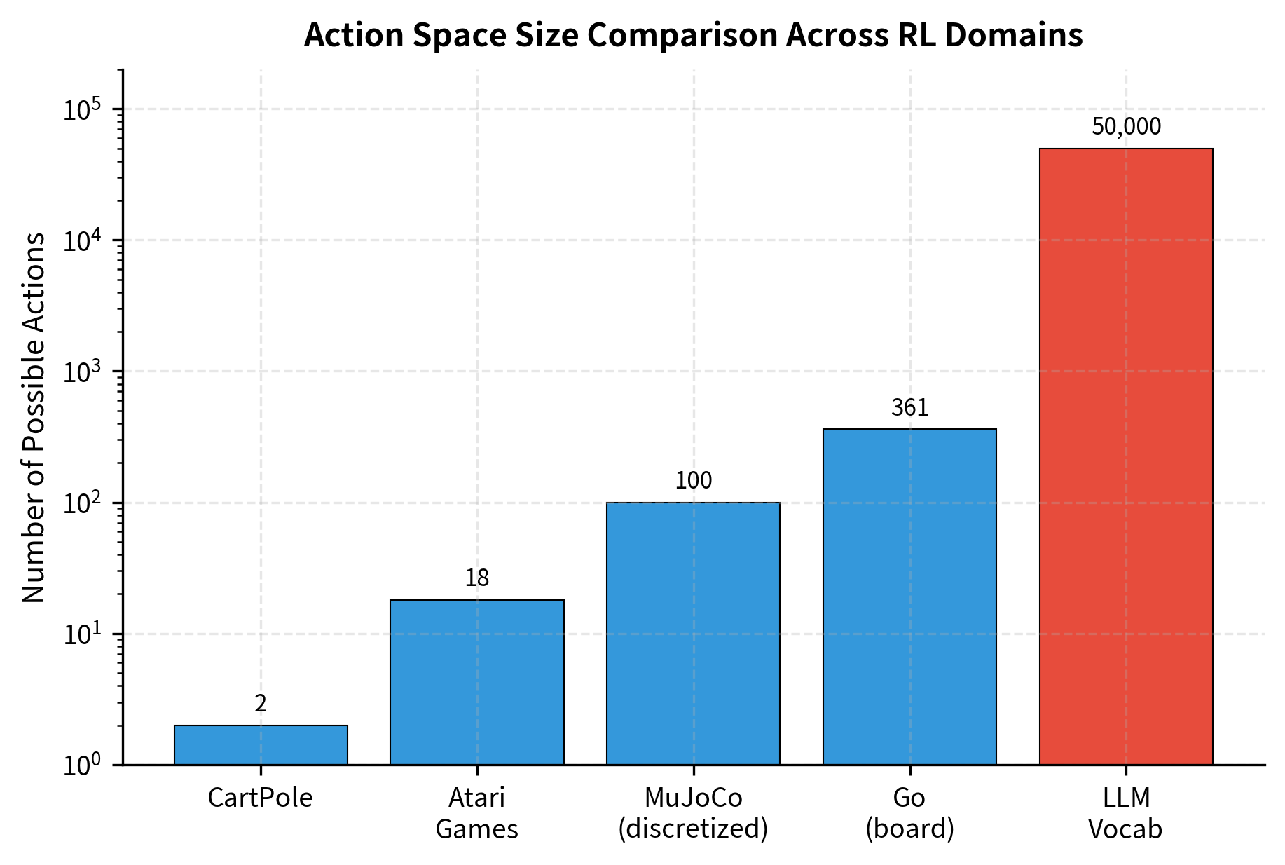
The action space in language generation is the model's vocabulary. This discrete set of tokens defines every possible action the policy can take at each step. Unlike continuous control problems where actions might be forces or velocities, or even discrete games where actions represent button presses, the language model's action space consists of linguistic units. These might be complete words, word fragments, punctuation marks, or special tokens that signal the end of generation.

For modern language models, this vocabulary typically contains between 30,000 and 100,000 tokens. The exact size depends on the tokenization algorithm used during pretraining. Byte-pair encoding, the most common approach, creates vocabularies that balance coverage of common words with the ability to represent rare words through subword decomposition. The vocabulary must be large enough to efficiently represent common text patterns while remaining small enough for the softmax computation to be tractable.

This scale is much larger than traditional RL domains. In classic control, action spaces are small. For example, a robot arm might have six joints. In Atari games, agents choose among roughly 18 discrete actions representing joystick directions and button combinations. Language models must select from tens of thousands of possible tokens at every single step. This represents an increase of three to four orders of magnitude in the number of discrete choices.

This has significant implications:

• Exploration is implicit: With such a large action space, the model cannot systematically try all options. There is no way to enumerate the consequences of every possible token choice. Instead, exploration emerges from the inherent stochasticity of sampling from high-entropy distributions during generation. When the model is uncertain, it assigns probability mass to many tokens, and sampling naturally explores these alternatives.
• Credit assignment is diffuse: When a response receives a reward, determining which specific token choices contributed to that reward is challenging. Did the response succeed because of word choice in the third sentence, or the overall argument structure? The signal must somehow propagate back through dozens or hundreds of individual decisions.
• Probability mass spreads thin: Even well-trained models may assign relatively small probabilities to any single token, making log probability computations numerically sensitive. When probabilities are small, their logarithms become large negative numbers, requiring careful numerical handling.

Despite these challenges, the discrete nature of the action space simplifies some aspects of PPO. We can compute exact action probabilities rather than approximating them, as we would need to do in continuous action spaces. We can directly enumerate the KL divergence between policies by summing over vocabulary positions. The softmax function gives us a proper probability distribution that sums to one, avoiding the density estimation challenges that arise with continuous distributions.

Each position in the generated sequence requires selecting from this massive action space. A 100-token response involves 100 sequential decisions, each choosing among 32,000 options. Even a short response spans a massive search space. This is why language generation uses learned policies to find good text efficiently.

The state in language generation grows with each action. Unlike a game where the agent might return to previously visited states, or a robot navigation task where the agent can revisit locations, language generation always moves forward. Each generated token permanently extends the context. The state at step $t+1$ contains everything from state $t$ plus the newly generated token.

Formally, the state at step $t$ is:

where:

• $s_t$: the state at timestep $t$
• $x_i$: the $i$-th token of the prompt
• $n$: the number of tokens in the prompt
• $y_j$: the $j$-th generated token

This formulation captures the essential nature of autoregressive generation. The state is not a compact summary of the situation; it is the complete history of what has been written. The model must condition on all of this information to decide what should come next. A word that appeared ten sentences ago might be crucial for maintaining coherence, while a word from three tokens ago might determine grammatical constraints on the current position.

This means the state space is infinite and largely unique to each trajectory. Two different prompts lead to entirely different state spaces, and even the same prompt with different generation paths explores different states. Unlike board games where states might repeat (the same chess position can arise from different move orders) or continuous control where the system might return to similar configurations, language generation creates fresh territory with every token. Each state is a unique point in the space of possible text prefixes.

The growing state affects implementation. The model must process longer sequences as it generates tokens. Each new token requires attending to all previous tokens, which increases computation quadratically. This is where techniques like KV caching, which we will cover in Part XXVIII, become essential for efficient inference and training. By storing key and value projections, the model avoids recomputing them. This changes complexity from quadratic to linear.

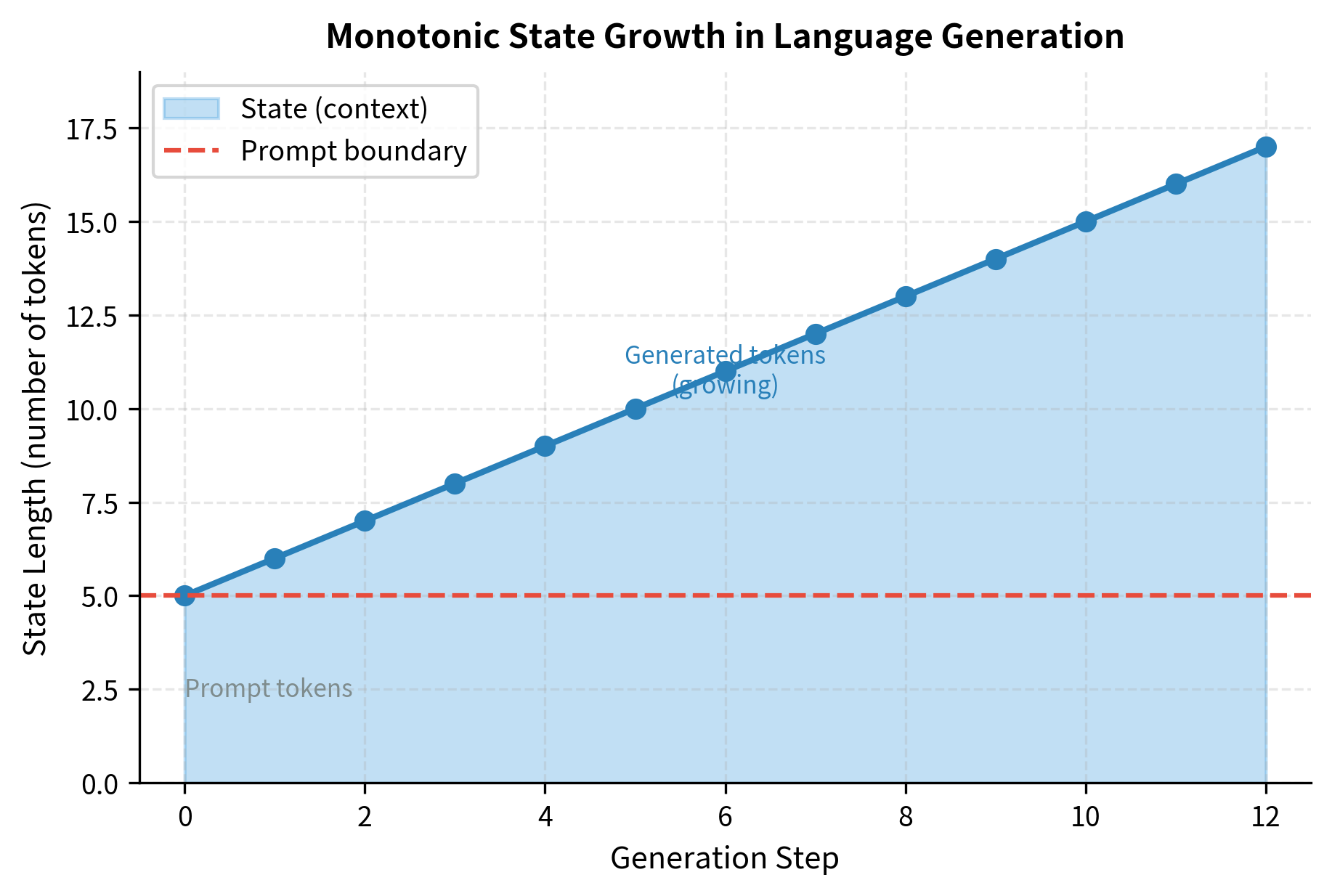
The generated trajectory illustrates how the context (state) expands with each step. Even a short response creates a sequence of unique states, as the growing history fundamentally changes the input to the policy at every decision point. At step 0, the policy sees only the prompt. At step 1, it sees the prompt plus one generated token. By the final step, it sees the entire conversation history. This expansion means that the policy faces a different decision problem at every timestep, even though the underlying question remains the same.

Reward models and RL algorithms use rewards differently, which creates challenges for PPO. The reward model, as we discussed in the chapter on Reward Modeling, takes a complete prompt-response pair and outputs a single scalar score. It evaluates the response as a whole, considering factors like helpfulness, coherence, accuracy, and safety. But PPO operates on trajectories with per-timestep rewards. The algorithm expects to receive a reward signal at each step, allowing it to compute advantages and update the policy accordingly.

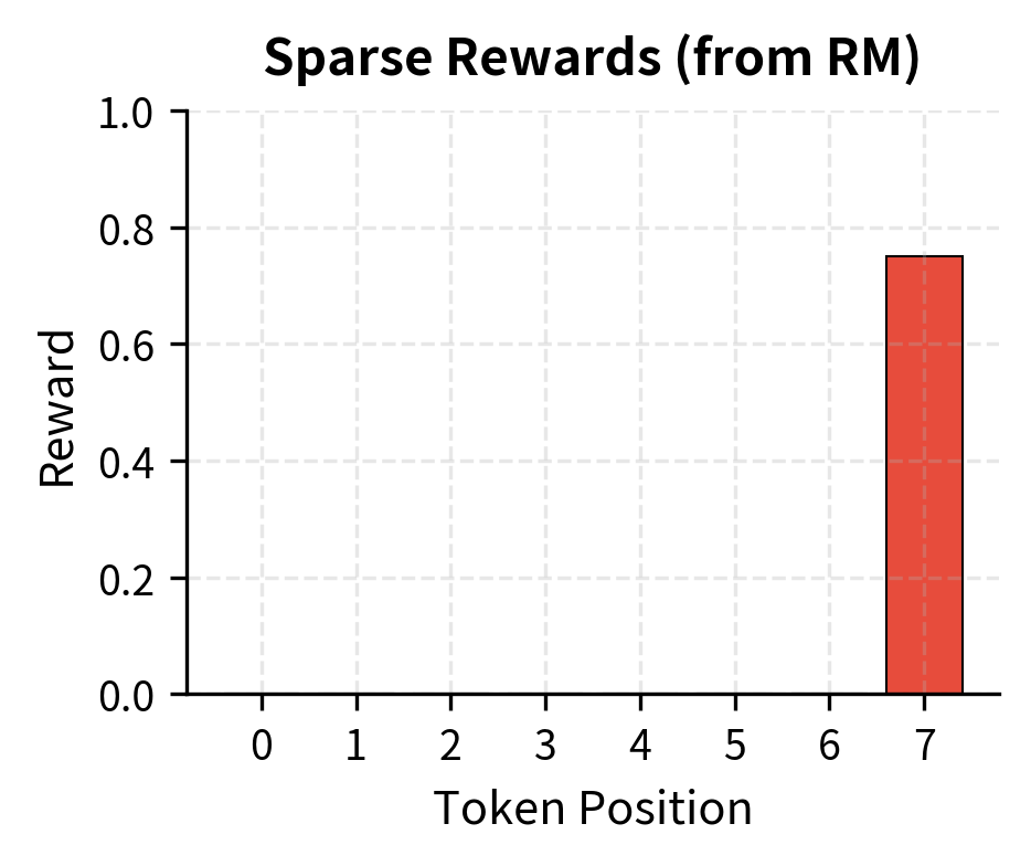
The standard approach assigns the reward to the final token:

where:

• $r_t$: the reward assigned at step $t$
• $R(x, y)$: the scalar score from the reward model for the complete response
• $T$: the length of the generated sequence (final step)
• $x$: the input prompt
• $y$: the complete generated response

This approach reflects that we only know how good a response is once it is complete. We usually cannot evaluate a partial response because quality depends on the full response and the final answer. So we wait until generation finishes, compute the reward, and assign it to the final step.

Sparse rewards make credit assignment difficult. The policy must learn which of its many token choices contributed to the final reward. PPO addresses this through its advantage estimation, but the challenge remains significant. A response might receive a low reward because of a single poor word choice, but that signal must propagate back through dozens of preceding tokens. The value function must learn to predict, from any intermediate state, what the expected final reward will be. This prediction is what allows advantages to differentiate between tokens: some tokens lead to states with high expected rewards, others to states with lower expectations.

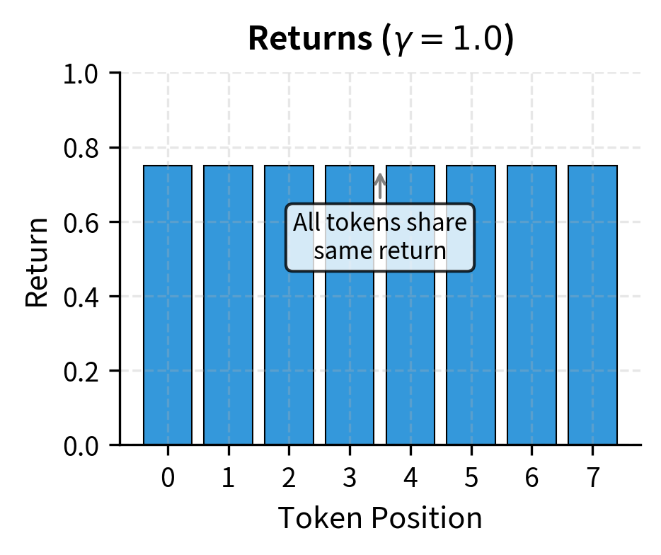
With a discount factor of $\gamma = 1.0$, which is standard in RLHF, every token in the sequence receives the same return, equal to the final reward. This uniform signal might seem uninformative at first glance. If every token gets the same return, how can the algorithm distinguish good tokens from bad ones? The answer lies in the advantage function, which compares the actual return to the expected return under the value function. A token that leads to a higher-than-expected return receives a positive advantage, while a token that leads to a lower-than-expected return receives a negative advantage. This differential signal, created by the value function's predictions, is what enables learning even with sparse rewards.

The most important adaptation for language model PPO is the KL divergence penalty. This constraint measures how far the policy drifts from its starting point and serves several purposes. Without this constraint, the optimized policy can diverge dramatically from the original model, often finding degenerate solutions that maximize reward without producing genuinely useful responses.

Without the KL penalty, the policy often finds degenerate solutions. The policy is free to move anywhere in the space of possible token distributions. If the reward model has any exploitable patterns, any shortcuts that yield high scores without genuine quality, the unconstrained policy will find them. It might learn to generate repetitive phrases that the reward model scores highly. It might produce outputs that superficially resemble good responses while lacking substance. It might drift so far from natural language that it generates text no human would write. The KL penalty prevents these failure modes by keeping the policy anchored to the reference distribution.

The KL penalty modifies the reward at each timestep:

where:

• $\tilde{r}_t$: the shaped reward at step $t$ used for PPO training
• $r_t$: the original sparse reward
• $\beta$: the KL penalty coefficient
• $\text{KL}_t$: the KL divergence contribution at this step

The KL term is defined as the log-ratio between the current policy and a reference policy:

where:

• $\pi_\theta(y_t | s_t)$: the probability of the chosen token under the current policy
• $\pi_{\text{ref}}(y_t | s_t)$: the probability of the chosen token under the reference policy
• $y_t$: the token generated at step $t$
• $s_t$: the context (state) at step $t$

This formula is easy to interpret. When the current policy assigns higher probability to a token than the reference did, the log ratio is positive, and the policy is penalized. When the current policy assigns lower probability, the log ratio is negative, and the policy receives a bonus. The net effect is that the policy is discouraged from making dramatic probability changes in either direction. It can shift probabilities to improve reward, but only within bounds.

The reference policy $\pi_{\text{ref}}$ is typically the model after supervised fine-tuning (SFT) but before any RL training. This anchor prevents the policy from drifting into regions of token space that the original model considered highly unlikely. The SFT model represents our best current understanding of how to generate helpful, coherent text. By constraining the RL policy to stay near this baseline, we ensure that the optimized model retains the linguistic competence learned during pretraining and SFT.

The coefficient $\beta$ controls the strength of this constraint. Higher values keep the policy closer to the reference but limit learning; the policy cannot deviate much even when doing so would improve reward. Lower values allow more exploration but risk instability and reward hacking; the policy might find degenerate solutions that maximize reward while producing poor text. Success in RLHF depends on finding the right balance. We will explore the mathematical properties and tuning of this penalty in detail in the upcoming chapter on KL Divergence Penalty.

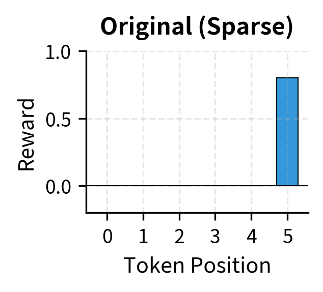
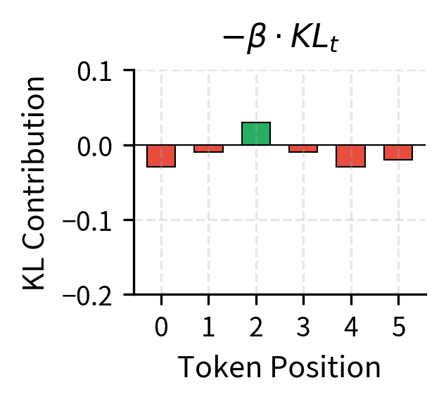
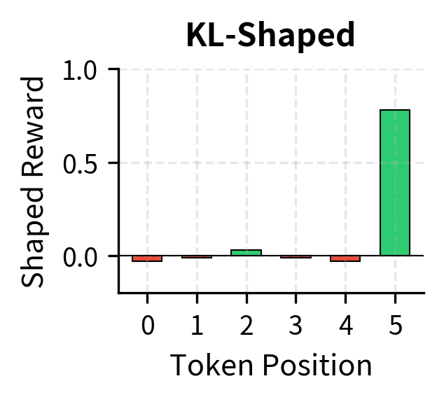
Notice how the KL penalty transforms the reward signal. The original sparse reward only provides signal at the final token; all intermediate tokens receive zero reward. After KL shaping, every token receives a reward component based on how much the policy diverges from the reference. Tokens where the policy assigns higher probability than the reference receive penalties (the KL term is positive, so it subtracts from the reward). Tokens where the policy assigns lower probability than the reference receive bonuses (the KL term is negative, so subtracting it adds to the reward). This transformation converts the sparse terminal reward into a dense per-token signal that guides the policy at every step.

Combining all these elements, the PPO objective for language models takes the following form. The PPO objective maximizes the expected advantage while keeping the policy close to its starting behavior. The clipping mechanism prevents destructively large updates that could destabilize training. For a batch of prompt-response pairs, we compute:

where:

• $\theta$: the parameters of the language model being optimized
• $\mathbb{E}_{(x,y) \sim \pi_{\theta_{\text{old}}}}$: the expectation over trajectories generated by the policy that collected the data
• $\rho_t(\theta)$: the probability ratio between the current and old policies at step $t$
• $\hat{A}_t$: the estimated advantage at step $t$, indicating how much better the chosen action was compared to the average
• $T$: the length of the generated sequence
• $\epsilon$: the clipping parameter (typically 0.1 or 0.2) that defines the trust region

The min operator serves a crucial purpose in this objective. It takes the conservative lower bound between the unclipped and clipped objectives, ensuring that updates cannot be too aggressive. If the advantage is positive, indicating that the chosen action was better than expected, clipping limits how much we increase the probability of the action. If the advantage is negative, indicating the action was worse than expected, clipping limits how much we decrease the probability. This prevents large updates that could collapse the policy.

The probability ratio $\rho_t(\theta)$ is defined as:

where:

• $\pi_\theta(y_t | x, y_{<t})$: the probability of the token $y_t$ under the current policy (being updated)
• $\pi_{\theta_{\text{old}}}(y_t | x, y_{<t})$: the probability of the same token under the policy that collected the data (frozen for this update step)
• $y_t$: the token generated at step $t$
• $x$: the input prompt
• $y_{<t}$: the sequence of tokens generated prior to step $t$

This ratio measures how the policy has changed since the data was collected. A ratio of 1.0 means the policy assigns exactly the same probability as before. A ratio greater than 1 means the policy now assigns higher probability to this token. A ratio less than 1 means the probability has decreased. By basing updates on this ratio rather than directly on log probabilities, PPO can perform multiple gradient steps on the same batch of data without the policy drifting too far from the data-collection policy.

The advantage $\hat{A}_t$ is estimated using GAE (Generalized Advantage Estimation) applied to the KL-shaped rewards:

where:

• $\gamma$: the discount factor (usually near 1.0 for RLHF)
• $\lambda$: the GAE smoothing parameter (typically 0.95)
• $T$: the length of the generated sequence
• $\delta_{t+l}$: the temporal difference (TD) error at step $t+l$

This summation calculates an exponentially weighted average of future TD errors. The parameter $\lambda$ controls the bias-variance trade-off: higher values rely more on observed returns (reducing bias but increasing variance), while lower values rely more on value estimates (reducing variance but potentially introducing bias from imperfect value predictions). Setting $\lambda = 1$ recovers Monte Carlo returns, while $\lambda = 0$ gives pure one-step TD learning. The typical value of 0.95 balances these considerations.

The TD error $\delta_t$ measures the surprise at each step: the difference between the observed reward plus the estimated value of the next state, and the estimated value of the current state:

where:

• $\tilde{r}_t$: the KL-shaped reward at step $t$
• $\gamma$: the discount factor
• $V(s_t)$: the value function estimate for state $s_t$
• $V(s_{t+1})$: the value function estimate for the next state (defined as 0 if $t=T$)

The TD error captures whether the transition was better or worse than expected. If the reward plus next-state value exceeds the current-state value, the transition was unexpectedly good, and the TD error is positive. If the sum falls short, the transition was unexpectedly bad, and the TD error is negative. These signals, accumulated through GAE, produce advantage estimates that indicate which actions led to better outcomes than the value function predicted.

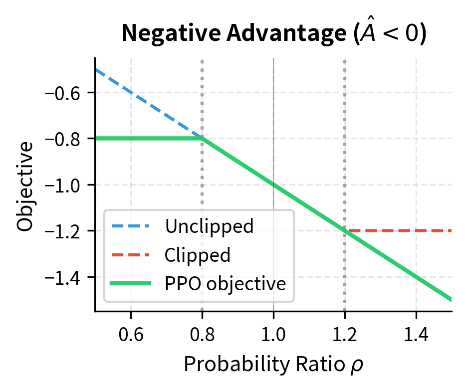
The positive advantage at the final step reflects the high reward, while negative values indicate steps that yielded lower-than-expected value. The probability ratios stay within the trust region defined by the clipping parameter, demonstrating how PPO maintains stability. When a ratio exceeds 1 + $\epsilon$ or falls below 1 - $\epsilon$, the clipped ratio takes over, preventing the gradient from pushing the policy further in that direction.

Let's now assemble a more complete implementation showing how these pieces fit together in a training step. This simplified version captures the essential structure while omitting some production details like distributed training, gradient accumulation, and advanced memory management. This example shows the flow of data and computation.

These hyperparameters define the constraints for the optimization. The clipping epsilon and KL coefficient are particularly critical for preventing the model from collapsing or drifting too far from its original capabilities. The value coefficient balances the policy and value function losses, and the GAE lambda controls the bias-variance trade-off in advantage estimation.

The following example demonstrates how PPO training proceeds at a high level. We use mock components to illustrate the data flow without requiring actual large models. This demonstration shows the essential rhythm of PPO training: generate responses, score them, compute advantages, and update the policy.

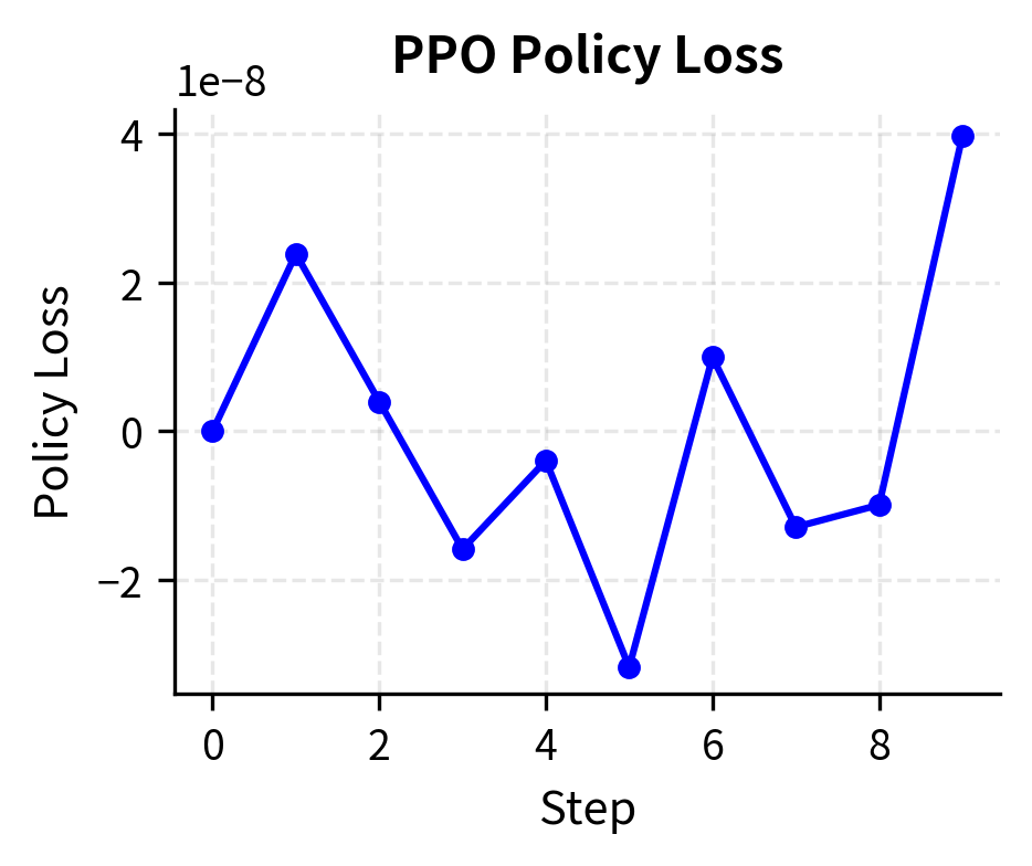
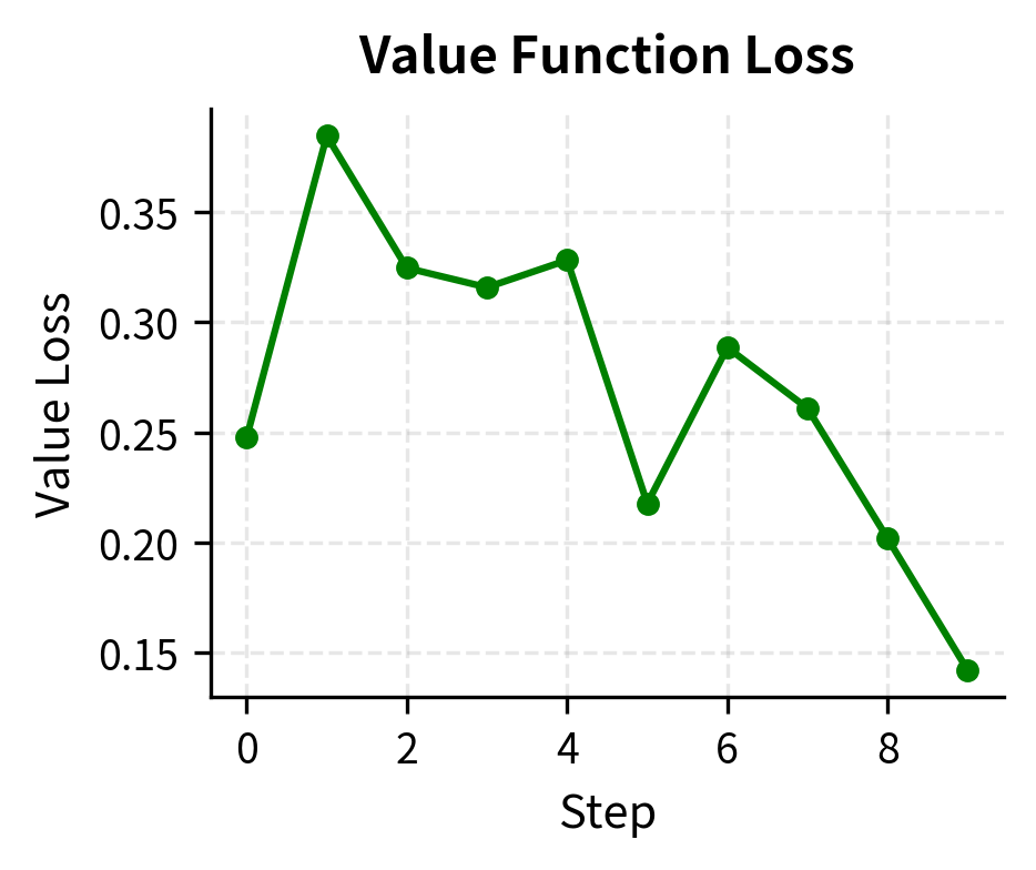
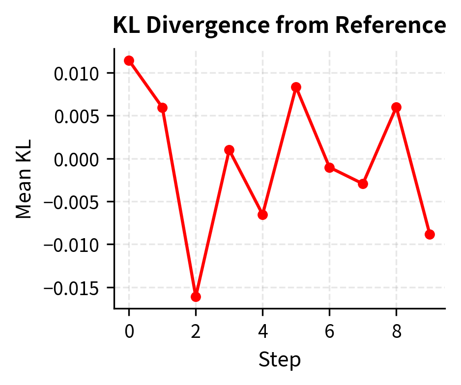
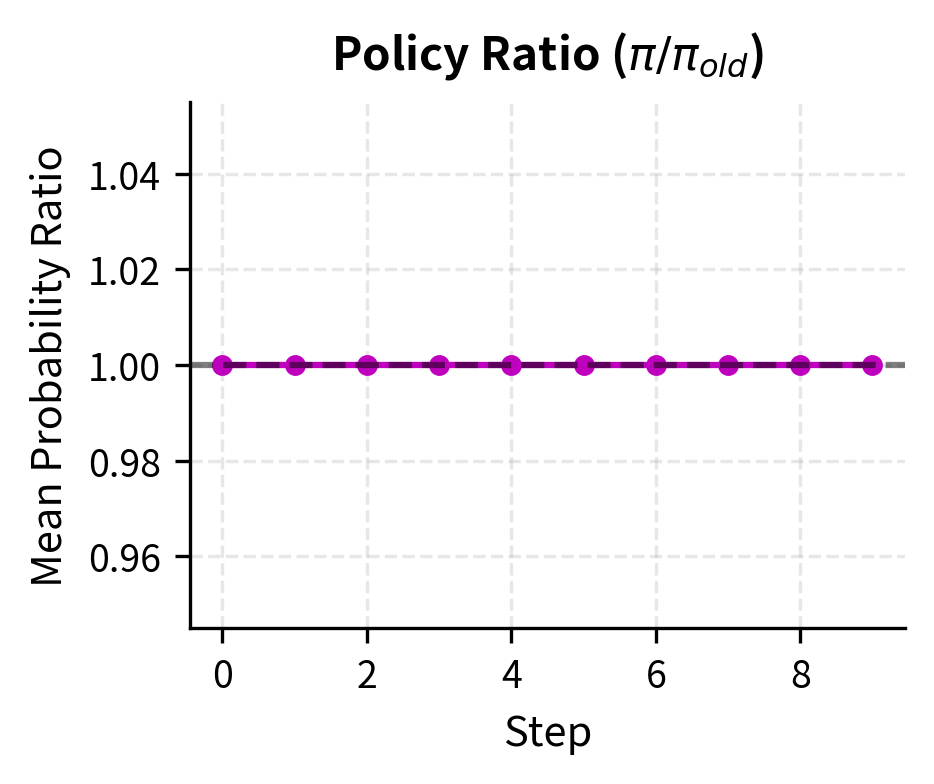
The training metrics reveal several important dynamics that you should monitor during real RLHF runs. The policy loss oscillates as the model learns to balance reward maximization against the clipping constraint. The KL divergence tracks how far the policy drifts from the reference, a key quantity we want to keep bounded. If KL grows too large, the policy is moving into territory where the reward model may not be reliable. The probability ratio stays near 1.0 because the clipping mechanism prevents extreme updates, demonstrating that the trust region constraint is functioning as intended.

The key parameters for PPO training are:

• clip_epsilon: The clipping threshold (typically 0.1 or 0.2) that constrains the policy update. Smaller values produce more conservative updates.
• kl_coef: Coefficient for the KL penalty term, controlling how closely the policy must stay to the reference model. This is perhaps the most important hyperparameter for preventing reward hacking.
• value_coef: Weight for the value function loss in the total optimization objective. Balancing this against the policy loss affects how quickly the value function adapts.
• gamma: Discount factor for future rewards. In RLHF, this is typically set to 1.0 since we care equally about all tokens in the response.
• lam: The GAE smoothing parameter that balances bias and variance in advantage estimation. Values around 0.95 are standard.

Implementing PPO for large language models involves several practical challenges beyond the algorithmic core. These engineering concerns often dominate the difficulty of real-world deployments and require careful attention.

Memory management is paramount. During training, you must store activations for the policy model, reference model, and value model simultaneously. The reference model can be loaded in half precision or quantized to reduce memory footprint. Some implementations share the backbone between policy and value models, adding only a small value head. This sharing reduces memory requirements but couples the representations, which may affect optimization dynamics.

Batch construction requires careful thought. Unlike supervised learning where examples are independent, PPO batches consist of complete generation trajectories. Generation is inherently sequential, making large-batch collection time-consuming. Implementations typically generate multiple responses in parallel across many prompts, using efficient batched inference to maximize throughput. The batch must contain enough diversity to provide a stable estimate of the gradient.

Response generation during training uses sampling rather than greedy decoding. This exploration is essential for PPO to discover high-reward responses that might differ from the reference policy's preferred outputs. Temperature and other sampling parameters become training hyperparameters that affect the exploration-exploitation balance. Too low a temperature leads to insufficient exploration; too high a temperature produces incoherent responses that receive low rewards.

Advantage normalization stabilizes training significantly. Normalizing advantages to have zero mean and unit variance across each batch prevents any single trajectory from dominating the gradient. Without normalization, a few outlier responses with extreme advantages could destabilize training by producing large gradient updates.

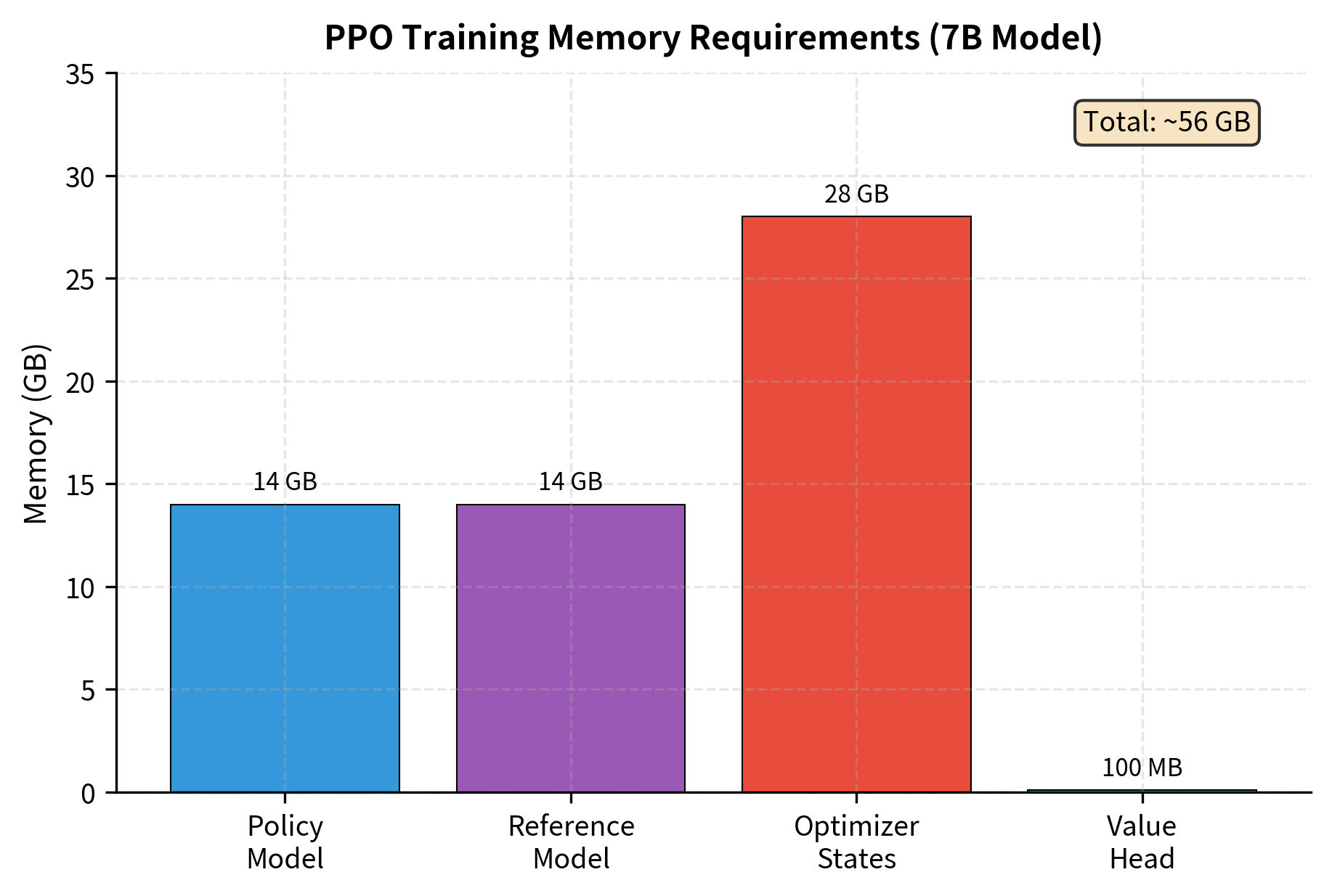
Optimization strategies:

• Load reference in 8-bit: saves ~7 GB
• Gradient checkpointing: reduces activation memory
• LoRA on policy: reduces optimizer state memory

Applying PPO to language models, while effective, comes with significant challenges that you must navigate. Understanding these limitations helps us find better methods.

Sparse rewards make credit assignment difficult. When a complete response receives a reward, determining which tokens contributed positively and which detracted is imprecise at best. The advantage function provides some differentiation through the value function's predictions, but it operates through imperfect estimates. The value function can only learn what patterns in intermediate states correlate with final rewards; it cannot directly observe the causal relationships. This imprecision can lead to slow learning, especially when the reward depends on subtle properties of the text that emerge from specific word choices or phrasings.

High computational cost is another barrier. PPO requires generating complete responses during training, which is much slower than the teacher-forcing paradigm used in supervised learning. Each training step involves running the policy model to generate text, running it again to compute log probabilities, running the reference model for KL computation, running the value model for advantage estimation, and running the reward model for scoring. Because of the computational and memory requirements, PPO is much more expensive than supervised fine-tuning. A single PPO training run can cost 10 to 100 times more than the equivalent SFT training.

The sensitivity to hyperparameters creates reproducibility challenges. The clipping parameter, KL coefficient, learning rate, and GAE parameters all interact in complex ways. Settings that work well for one model or task may fail on another. Small changes to any hyperparameter can lead to training instability or suboptimal results. This sensitivity motivates the development of alternative approaches, which we will explore in upcoming chapters on DPO and its variants.

Finally, the reliance on a learned reward model introduces all the challenges we discussed in the Reward Hacking chapter. The reward model is a proxy for human preferences, and optimizing it too aggressively can lead to responses that score highly according to the model while being less useful or even harmful. The KL penalty mitigates but does not eliminate this risk. Balancing reward optimization and constraints is an active research area.

This chapter translated the PPO algorithm from its general reinforcement learning formulation to the specific setting of language model alignment. The key conceptual mappings are:

• A language model serves as a stochastic policy, with states being the growing context and actions being vocabulary tokens
• The action space is the vocabulary, typically containing 30,000 to 100,000 discrete options
• Rewards are assigned sparsely, with the reward model's score appearing only at the final token
• The KL divergence penalty transforms sparse rewards into dense signal while preventing policy collapse

The PPO objective for language models combines the clipped surrogate loss with KL-shaped rewards, creating a training signal that balances reward maximization against staying close to the reference distribution. This balance is crucial for stable training and for avoiding reward hacking.

In the next chapter on the RLHF Pipeline, we will see how PPO fits into the complete workflow that transforms a pretrained language model into an aligned assistant, including the data collection, reward model training, and iterative refinement stages that surround the PPO optimization we have studied here.

Ready to test your understanding? Take this quick quiz to reinforce what you've learned about applying PPO to language models.