

Master iterative alignment for LLMs with online DPO, rolling references, Constitutional AI, and SPIN. Build self-improving models beyond single-shot training.

This article is part of the free-to-read Language AI Handbook
Choose your expertise level to adjust how many terms are explained. Beginners see more tooltips, experts see fewer to maintain reading flow. Hover over underlined terms for instant definitions.
Iterative Alignment
The alignment methods we've explored so far, such as RLHF, DPO, and their variants, typically treat alignment as a one-shot process. You collect preferences, train once, and deploy the model. But alignment is an ongoing challenge, not a single event. Models that seem well-aligned can drift as they encounter new situations, and static preference datasets quickly become outdated as the model's behavior evolves. This chapter explores iterative approaches to alignment, where models undergo multiple rounds of training with fresh preference data, sometimes generating that data themselves.
Iterative alignment is necessary because training a model on preference data changes its distribution. Its outputs no longer match the distribution that generated the original training examples. This creates a distribution mismatch that can degrade alignment quality over time. By iteratively collecting new preferences on the model's current outputs and retraining, we can maintain tighter alignment and even enable models to improve beyond what any single training run could achieve.
The Case for Iteration
Consider what happens in standard DPO training. You start with a reference model , collect human preferences comparing pairs of responses, and train the model to prefer the winning responses. After training, you have a new model that behaves differently from . But your training data was generated from , so it reflects the kinds of responses that model produced and the relative quality judgments between them.
To understand why this matters, imagine teaching someone to write by showing them examples of mediocre essays and asking them to identify which is slightly better. They might learn to avoid the worst mistakes, but they never see what excellent writing actually looks like. The training signal is fundamentally limited by the quality of the examples being compared. When your model improves beyond the capability level present in the training data, the preference comparisons become less informative because they no longer represent the kinds of decisions the improved model needs to make.
This creates several problems:
- Distribution mismatch: The preference comparisons were between responses from , but the model now generates different responses. The training signal becomes less relevant.
- Ceiling effects: If both responses in a preference pair are poor, learning to prefer the "less bad" option doesn't teach the model what a truly good response looks like.
- Static feedback: Human values and expectations evolve. A dataset collected once becomes stale.
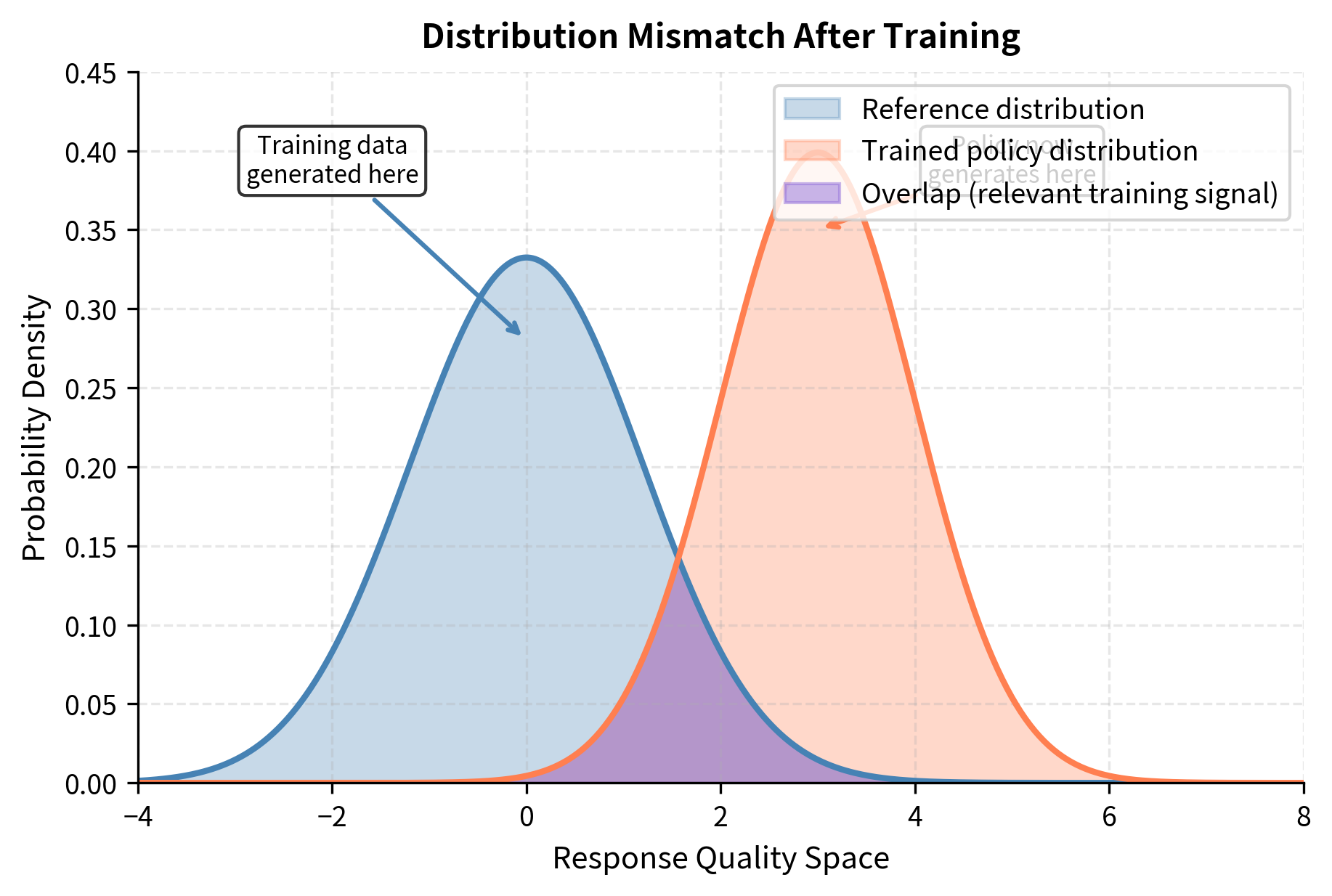
Distribution mismatch is the primary reason why iteration matters. When you train a model to prefer response A over response B, you are implicitly teaching it something about the boundary between good and bad responses in that region of output space. But after training, the model no longer generates responses in that same region. It has moved to a different part of the output distribution, where the old preference comparisons may not provide useful guidance. The model might now be generating responses that are uniformly better than anything in the original training set, or it might be making new types of errors that the original comparisons never addressed.
Iterative alignment addresses these issues by making alignment a continuous process. After each training round, we generate new responses from the updated model, collect fresh preferences, and train again. This keeps the training distribution matched to the current policy and allows the model to learn from increasingly sophisticated comparisons. Each iteration provides feedback on the model's actual current behavior, creating a feedback loop that can continuously refine alignment quality.
Iterative DPO
As we discussed in the DPO chapters, Direct Preference Optimization implicitly defines a reward function through the log-probability ratio between the policy and reference model. This mathematical relationship makes the reference model central to what DPO learns. The reference model serves as an anchor point that defines the baseline against which improvements are measured. When we iterate DPO, we have a choice: keep the original reference model fixed, or update it at each iteration. This choice significantly affects training dynamics and the final model's behavior.
Fixed Reference Iteration
The simplest form of iterative DPO keeps the original reference model fixed across all iterations. At each round , we generate responses from the current policy , collect preferences, and train to get . This approach maintains a consistent anchor point throughout the entire iterative process, always measuring progress relative to where the model started.
The loss at iteration becomes:
Unpacking the formula components clarifies how they guide iterative training:
- : the loss function minimized at iteration
- : the expectation operator averaging over all preference pairs in the dataset
- : the dataset of preferences collected from responses generated by the current policy
- : the policy model currently being trained (parameterized by )
- : the fixed reference model (usually the initial policy)
- : the input prompt
- : the winning and losing responses, respectively, for prompt
- : the logistic sigmoid function
- : the temperature parameter controlling the strength of the KL penalty
- : the implicit reward term (higher values indicate the policy is more likely to generate than the reference)
The key change from standard DPO is that contains preferences over responses generated by , not the original reference model. This subtle but crucial difference ensures the model learns from comparisons that reflect its current capabilities rather than from stale comparisons between outputs it no longer produces. The model receives feedback on the kinds of responses it actually generates now, making the training signal directly relevant to improving current behavior.
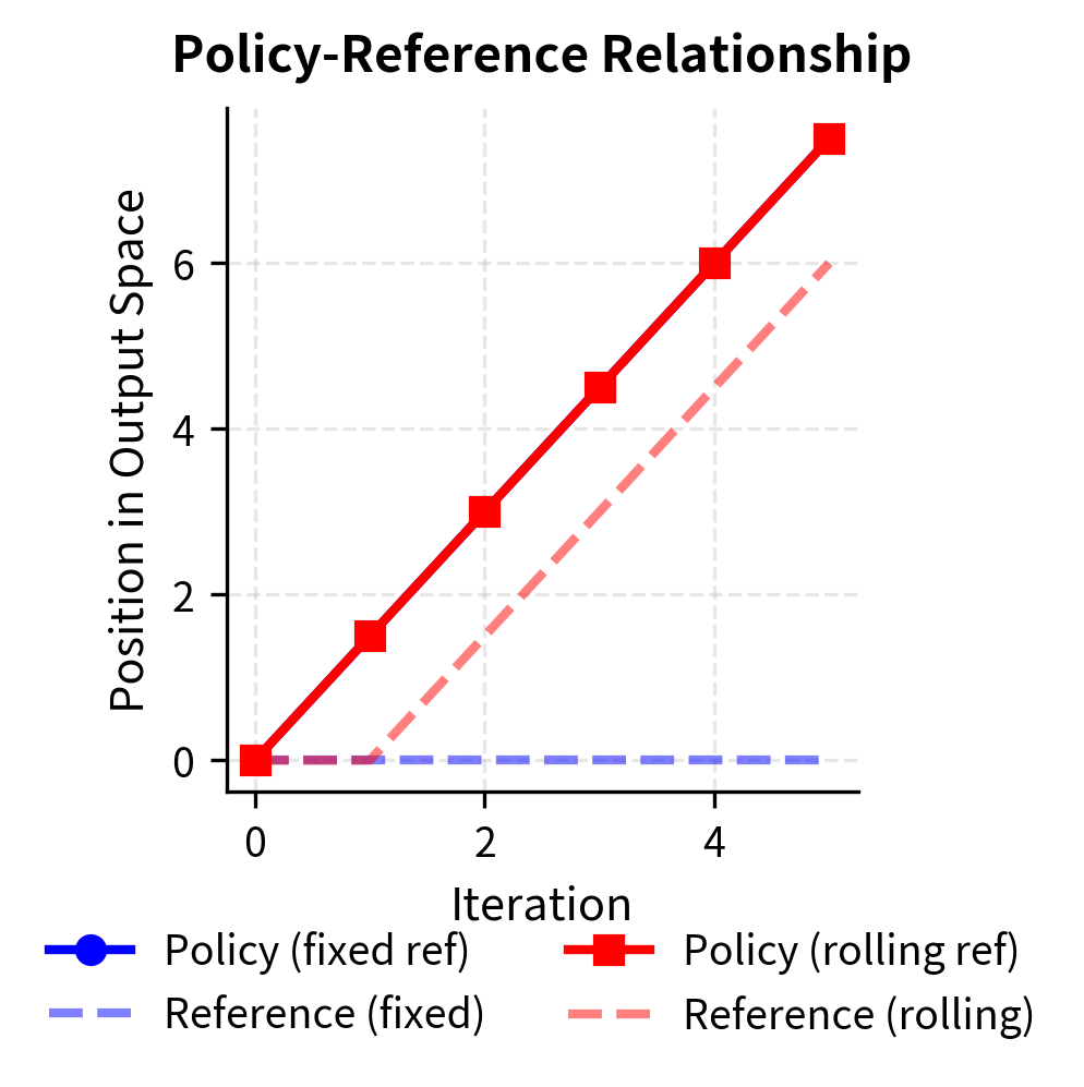
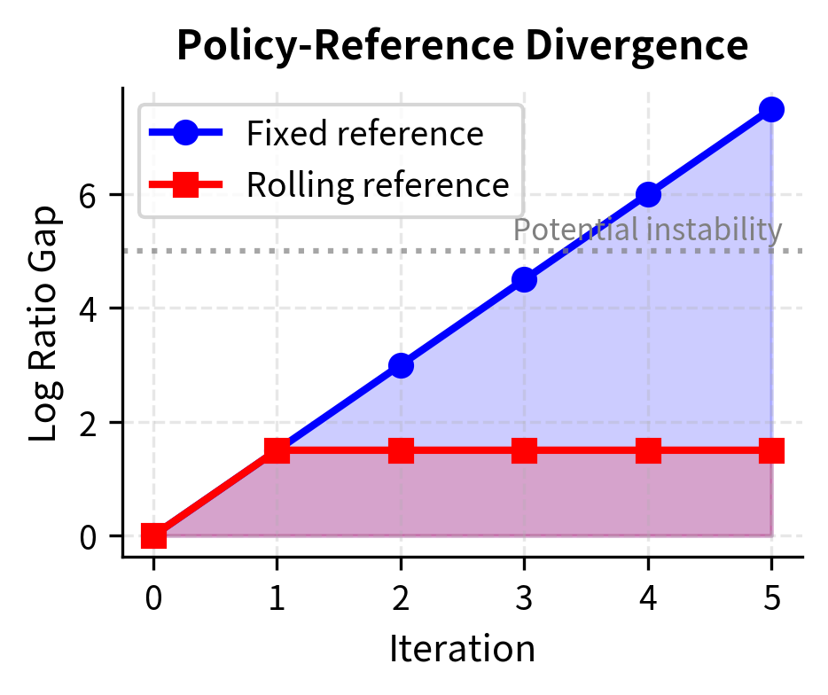
However, keeping a fixed reference creates a growing gap between the reference and policy distributions. As the policy improves over iterations, it diverges further from . The implicit reward function now compares very different distributions. When the policy assigns high probability to a response that the reference considers extremely unlikely, the log ratio becomes very large. Conversely, when the policy considers a response unlikely but the reference assigns moderate probability, the log ratio becomes very negative. These extreme values can destabilize training by creating large gradients that push the model erratically.
Rolling Reference Iteration
A more common approach updates the reference model at each iteration. After training round , we set before starting round . This keeps the reference close to the current policy, maintaining stable gradients and ensuring that the log probability ratios remain in a reasonable range throughout training.
The rolling reference focuses on incremental improvements instead of measuring progress against the initial model. By using the previous iteration's policy as the reference, we are essentially asking: "Given where we are now, which responses represent improvements?" This framing naturally prevents the extreme probability ratios that arise when comparing against a very different reference distribution.
The iterative procedure becomes:
- Initialize with a supervised fine-tuned model
- Set
- For each iteration :
- Generate responses from on a set of prompts
- Collect preferences over response pairs
- Train using DPO with reference
- Update
This rolling reference approach is sometimes called online DPO because the training data comes from the current policy rather than a static offline dataset. The term "online" here refers to the fact that data generation is interleaved with training, creating a dynamic feedback loop between model behavior and the training signal.
Rolling reference training starts from a neutral position. The policy and reference are identical at the beginning of each round, so the log probability ratios start at zero for all responses. This means the training signal comes entirely from the preference comparisons in the current iteration's dataset, without any accumulated bias from previous iterations. The model learns to improve relative to its immediate predecessor, and the cumulative effect of many such improvements can be substantial.
IPO for Iterative Training
Recall from our discussion of DPO variants that Identity Preference Optimization (IPO) avoids the length exploitation issues that can plague DPO over multiple iterations. The problem with standard DPO becomes particularly acute in iterative settings: if the model learns that slightly longer responses tend to win preference comparisons, it will generate longer responses, which will then be compared against each other, and the longest will again tend to win. This feedback loop can drive response length to extreme values over many iterations.
IPO addresses this concern through a fundamentally different objective formulation. Rather than using the sigmoid function to bound the preference probability, IPO directly targets a specific margin between the preferred and dispreferred log probability ratios. The IPO objective is:
The components of the IPO formula prevent the runaway behavior seen in DPO:
- : the Identity Preference Optimization loss
- : the expectation operator averaging over the dataset
- : the policy model being trained
- : the reference model
- : the input prompt
- : the preferred and dispreferred responses for prompt
- : the hyperparameter derived from the KL regularization strength
This objective minimizes the squared error between the log-likelihood ratio gap and a finite target margin of . The key insight is that IPO does not simply try to make the preferred response more likely than the dispreferred one; it tries to make the gap between them equal to a specific target value. Once the model achieves this target margin, further increasing the gap actually increases the loss. This built-in saturation prevents the model from pushing probability ratios to extreme values.
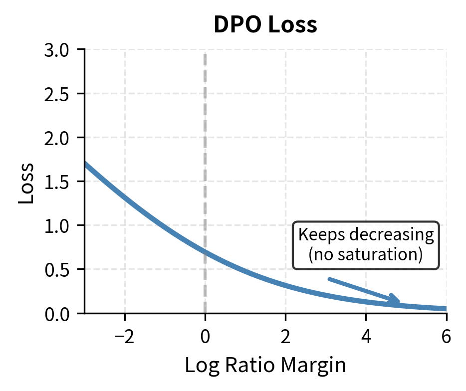
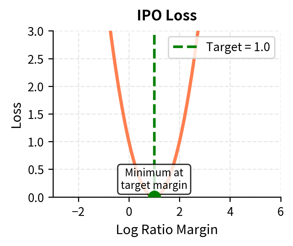
Unlike DPO, which tries to maximize the gap (bounded only by the asymptotic behavior of the sigmoid), IPO targets this specific margin, preventing the model from pushing probability ratios to extreme values. The squared error formulation means that overshooting the target margin is penalized just as much as undershooting it. This symmetric penalty structure provides natural regularization that becomes increasingly important over multiple iterations where small biases otherwise compound into significant distortions.
Online Preference Learning
The distinction between online and offline preference learning parallels the classic reinforcement learning distinction between on-policy and off-policy methods. This parallel is not merely superficial; the same fundamental trade-offs apply in both contexts, and understanding these trade-offs helps clarify when each approach is appropriate.
Offline methods use a fixed dataset of preferences collected once, typically from a different model or earlier version. Online methods generate fresh responses from the current policy and collect preferences on those responses during training.
In offline reinforcement learning, an agent learns from a fixed dataset of experiences collected by a different policy, perhaps a human expert or an earlier version of the agent. The challenge is that the agent cannot explore: it must learn entirely from the experiences provided. In offline preference learning, the situation is analogous. The model learns from preference comparisons between responses that were generated by some other model, and it cannot generate new responses to get feedback on during training.
Advantages of Online Learning
Online preference learning offers several benefits over offline approaches:
- Distribution matching: Training data always reflects the current policy's behavior
- Progressive difficulty: As the model improves, comparisons become more nuanced
- Adaptive exploration: The model can explore regions of response space that earlier versions couldn't reach
- Reduced overfitting: Fresh data prevents memorizing fixed preference patterns
Distribution matching directly addresses the motivation for iterative alignment. When training data comes from the current policy, every preference comparison provides information about choices the model is actually making. There is no disconnect between what the model generates and what the training signal evaluates. This tight coupling ensures that the training signal remains relevant throughout the optimization process.
Progressive difficulty emerges naturally from online learning. In early iterations, the model might generate responses with obvious quality differences, making preference judgments easy. As the model improves, the differences between its responses become more subtle, requiring more careful evaluation. This natural curriculum exposes the model to increasingly sophisticated distinctions, pushing it toward finer-grained improvements that offline data might not capture.
The major drawback is cost. Online learning requires generating new responses and obtaining preferences continuously, which can be expensive when using human annotators. Each iteration requires not just training time but also the time and resources needed to generate candidate responses and evaluate them. For organizations with limited annotation budgets, this ongoing cost can be prohibitive.
On-Policy Sampling Strategies
When generating responses for online preference learning, several sampling strategies exist, each with different trade-offs between sample efficiency, coverage, and computational cost:
Best-of-N sampling: Generate responses per prompt, use a reward model to select the best and worst, then train on this pair. This is sample-efficient but requires a reward model. The approach maximizes the information content of each preference pair by ensuring a substantial quality gap between the compared responses. However, it relies on the reward model's accuracy, and any systematic biases in the reward model will be amplified through this selection process.
Diverse sampling: Use different temperatures or sampling strategies to generate varied responses, ensuring the preference pairs cover diverse regions of response space. Higher temperatures produce more varied outputs, potentially exposing the model to a broader range of quality levels. This approach reduces the risk of overfitting to a narrow slice of the output distribution but may produce many comparisons between clearly bad responses, which provide limited learning signal.
Targeted sampling: Focus on prompts where the model's current responses are uncertain or low-quality, similar to active learning approaches. By directing annotation effort toward the most informative examples, this strategy can achieve better sample efficiency than random sampling. The challenge lies in identifying which prompts will yield the most useful preference comparisons without actually collecting those comparisons first.
Converting RLHF to Online DPO
The RLHF pipeline we covered earlier is inherently online: PPO samples from the current policy and updates based on reward model scores. We can convert this to online DPO by:
- Generating pairs of responses from the current policy
- Using the reward model to determine preferences (instead of providing scalar rewards)
- Training with DPO instead of PPO
This hybrid approach, sometimes called reward model distillation or RLHaF (Reinforcement Learning from Human-AI Feedback), combines the stability of DPO with the online sampling of RLHF. The key insight is that a reward model can be used to generate preference labels rather than to provide direct reward signals. By converting scalar rewards into binary preference comparisons, we can use the simpler DPO training procedure while retaining the benefits of online data generation.
This conversion is practical because DPO is more stable and easier to tune than PPO. By using the reward model only to generate preference labels rather than to guide policy gradient updates, we sidestep many of the challenges that make RLHF difficult in practice.
Self-Improvement Loops
Iterative alignment enables self-improvement, where models generate their own training data to improve without human annotation. This sounds almost paradoxical: how can a model teach itself to be better than it already is? The answer lies in understanding the asymmetry between different cognitive tasks.
The Self-Improvement Paradox
Self-improvement relies on the fact that evaluating responses is easier than generating them. A model might struggle to write a perfect response but can often tell which of two responses is better. By generating many candidates, evaluating them, and training on the best, the model can improve beyond its initial capabilities.
This asymmetry is fundamental to many human learning processes as well. Consider a chess player analyzing their games: they might not be able to find the best move during play, but with time to reflect, they can often identify which of their moves were mistakes. The evaluation task, with its reduced time pressure and ability to compare alternatives, is genuinely easier than the generation task of finding the best move under tournament conditions.
This is analogous to how humans learn. A student might not be able to write a great essay from scratch but can recognize quality when comparing examples. Through exposure to what makes one response better than another, they gradually internalize those standards. The model undergoes a similar process: by repeatedly seeing which of its outputs are preferred, it learns to generate responses with those preferred characteristics more reliably.
The self-improvement loop works because the model effectively bootstraps from its ability to recognize quality to its ability to generate quality. Each iteration tightens this connection. The model generates candidates that reflect its current generation capabilities, evaluates them using its (potentially superior) evaluation capabilities, and trains on the resulting preferences to improve its generation capabilities. The cycle then repeats with a now-improved generator.
Constitutional AI
Anthropic's Constitutional AI (CAI) pioneered practical self-improvement for alignment. The approach works in two phases:
Critique and revision phase: The model generates a response, then critiques it according to a set of principles (the "constitution"), then revises the response to address the critique. This creates pairs of (original, revised) responses.
Preference learning phase: The revised responses are treated as preferred over the originals, creating synthetic preference data for DPO or RLHF training.
The constitution might include principles like:
- "Please choose the response that is most helpful while being harmless and honest."
- "Please choose the response that is least likely to cause harm if misused."
- "Please choose the response that best follows your instructions while refusing harmful requests."
Following explicit principles is easier than inferring human preferences. When a model must infer human preferences from examples, it faces an ambiguous learning problem: many different underlying value functions could explain the observed preferences. But when principles are stated explicitly, the model has clear criteria to apply. By making the criteria explicit, the model can self-critique more reliably, identifying specific ways in which a response violates stated principles and revising accordingly.
Constitutional AI also addresses the scalability challenge of human annotation. Collecting human preferences is expensive and slow. By using explicit principles that the model can apply to its own outputs, CAI dramatically reduces the need for human involvement in each training iteration. Humans still play a crucial role in defining the constitutional principles, but the actual preference generation scales with compute rather than with human annotator time.
Self-Play Fine-Tuning (SPIN)
Self-Play Fine-Tuning takes a different approach to self-improvement. Instead of critique and revision, SPIN uses the model's own outputs as negative examples:
- Take a prompt and ground-truth response (from supervised data)
- Generate a response from the current model
- Create a preference pair: where is preferred
- Train with DPO to prefer over
The ground-truth response should be at least as good as current model generations. By training to prefer , the model moves toward the data distribution while exceeding its current capabilities. This approach requires no external judge or reward model; the ground-truth data itself provides the quality signal.
As training progresses, the model's outputs improve, so the contrast between and decreases. This naturally creates a curriculum: early iterations provide strong gradients (when model outputs are poor), while later iterations fine-tune on subtle differences. The learning signal adapts automatically to the model's current capability level without any explicit curriculum design.
The SPIN approach has an elegant theoretical interpretation. At convergence, the model should generate responses indistinguishable from the ground-truth distribution. If the model's outputs matched the ground-truth distribution perfectly, the preference pairs would be between equally good responses, providing no learning signal. The training naturally terminates when the model achieves the quality level of the ground-truth data.
LLM-as-Judge
A powerful approach for synthetic preference generation uses a language model itself as the preference judge. Given two responses, a judge model determines which is better, often with explanations.
The judge can be:
- The same model being trained (self-judgment)
- A larger, more capable model (teacher-student)
- A specialized critic model trained for evaluation
As we discussed in the RLAIF chapter, using AI feedback can scale alignment annotation significantly. In iterative settings, this enables rapid generation of preference data without human bottlenecks. A single GPU can generate thousands of preference judgments in the time it would take a human annotator to evaluate dozens.
However, self-judgment introduces risks. The model might develop blind spots that it can't recognize in its own outputs. If the model consistently makes a particular type of error, it may also consistently fail to identify that error when judging its outputs. Using an external judge model or periodically incorporating human feedback helps maintain calibration and prevents the accumulation of systematic biases over iterations.
Alignment Stability
Iterative training introduces failure modes that don't appear in single-round alignment. Understanding these is crucial for building robust iterative systems that improve reliably rather than degrading in subtle ways over time.
Distribution Shift and Model Collapse
Over many iterations, the model's output distribution can shift dramatically from where it started. Small biases in the preference signal accumulate, potentially leading to model collapse: the model produces homogeneous outputs that score well on the preference metric but lack diversity or quality.
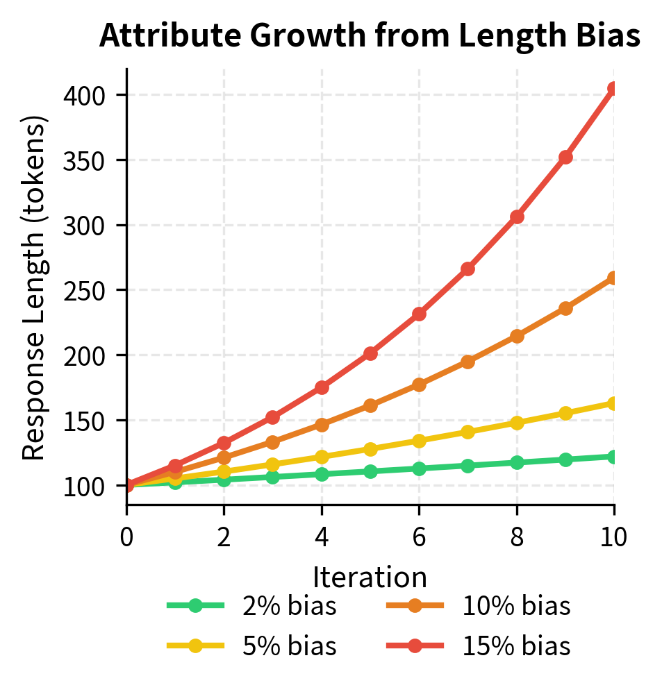
To understand how model collapse occurs, consider the dynamics of iterative training with a slightly biased preference signal. Suppose the judge model has a subtle preference for longer responses. In the first iteration, this bias causes the model to learn that somewhat longer responses are preferred. In the second iteration, the training data consists of these somewhat longer responses, and the judge again prefers the longest among them. The model learns to generate even longer outputs. This process continues iteration after iteration, with each round amplifying the length bias.
Consider a judge model that slightly prefers longer responses. Over iterations, the policy learns to generate longer outputs. These longer outputs are compared against each other, and the judge still prefers the longest. The model's outputs grow unboundedly, eventually becoming verbose and unhelpful.
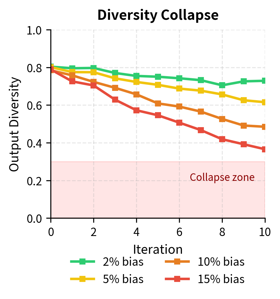
Similar collapse can occur along other dimensions: formality, hedging, particular phrasings. Any small consistent bias in evaluation compounds over iterations. A slight preference for confident-sounding language can evolve into overconfident assertions. A slight preference for hedged statements can produce responses so qualified that they become uninformative. The iterative process acts as an amplifier for whatever biases exist in the evaluation signal.
Mitigations include:
- Diversity penalties: Explicitly encourage varied outputs during generation
- Length normalization: Prevent length-based gaming
- Regular human evaluation: Catch drift before it compounds
- KL penalties: Keep the policy close to a fixed reference
Reward Hacking Accumulation
As we discussed in the Reward Hacking chapter, models can exploit gaps between what the reward signal measures and what we actually want. In iterative settings, this becomes more severe because each iteration builds on the potentially compromised foundation of previous iterations.
Each iteration might introduce a small amount of reward hacking. The next iteration's preference data comes from this slightly-hacked model, so the hacking becomes embedded in the training distribution. The next round of training builds on this compromised foundation, potentially amplifying the exploit. What starts as a barely noticeable tendency can grow into a dominant behavior pattern over many iterations.
For example, if the reward model has a small blind spot around sycophantic responses, early iterations might learn slight sycophancy. Later iterations generate training data that normalizes this behavior, making the model more confidently sycophantic, which the reward model continues to miss. The model learns that agreeing with you leads to positive feedback, then learns that emphatic agreement leads to even more positive feedback, eventually producing responses that are effusively agreeable regardless of whether your statements are accurate.
Breaking this cycle requires:
- Diverse reward signals: Use multiple reward models or judges with different biases
- Human oversight: Periodically inject human preferences to correct drift
- Adversarial probing: Actively search for behaviors the reward might miss
Capability Degradation
A subtle failure mode in iterative alignment is capability degradation or alignment tax. As the model learns to satisfy preferences, it might lose general capabilities that weren't directly measured. The training process optimizes what is measured, and capabilities that are not included in the preference signal may deteriorate.
For instance, iterative training focused on helpfulness might degrade the model's performance on factual recall or mathematical reasoning. The model becomes very good at sounding helpful but loses substance. If the preference comparisons rarely involve questions requiring precise factual knowledge, the model has no training signal to maintain that capability. Meanwhile, the weight updates that improve helpfulness may interfere with the representations that support factual recall.
This occurs because:
- Training updates push the model toward preference-satisfying regions of parameter space
- These regions may not preserve all pretrained capabilities
- Iterative training compounds these small capability losses
The compounding effect is particularly concerning. A 1% capability loss per iteration might seem acceptable, but after 50 iterations, the cumulative loss becomes substantial. Capabilities that were strong in the initial model may become unreliable in the final model, even though no single iteration caused dramatic degradation.
Monitoring diverse capabilities (not just alignment metrics) across iterations helps detect this. Many teams incorporate capability benchmarks into their iterative training loops, halting or reverting training if key capabilities degrade.
Reference Model Choice
The choice of reference model significantly impacts iterative stability. Using a rolling reference (updating each iteration) keeps gradients stable but allows unbounded drift from the original model. Using a fixed reference maintains a consistent anchor but can create increasingly large probability ratios that destabilize training.
Each choice involves trade-offs. The rolling reference provides a stable optimization landscape at each iteration, since the policy and reference start close together. But there is no mechanism preventing the policy from drifting arbitrarily far from the initial model over many iterations. The fixed reference prevents such drift by always measuring progress relative to the same anchor, but as the policy improves, the growing divergence between policy and reference creates numerical challenges.
A hybrid approach uses a fixed distant reference with a soft KL penalty plus a rolling recent reference for DPO:
The combined loss function includes these terms:
- : the combined hybrid loss function
- : the standard DPO loss calculated using the rolling reference
- : the current policy model
- : the reference model updated at each iteration (usually )
- : the weighting coefficient for the fixed reference KL term
- : the Kullback-Leibler divergence
- : the static reference model (usually )
This provides stable gradients from the rolling reference and bounded drift from the fixed anchor. The DPO loss provides the primary training signal, using the rolling reference to ensure reasonable probability ratios. The KL penalty term acts as a soft constraint, allowing the policy to improve beyond the initial model while preventing extreme divergence. The weighting coefficient controls the strength of this anchoring effect, with larger values keeping the policy closer to the original model at the cost of potentially limiting improvement.
Implementation
Let's implement an iterative DPO training loop that demonstrates these concepts. We'll simulate preference data generation and show how to structure multiple training rounds.
First, we'll create a simple language model for demonstration purposes. In practice, you'd use a full transformer, but this captures the key dynamics.
Now let's define the DPO training components.
We need a simulated preference oracle. In practice, this would be human annotators or a reward model. Our oracle prefers sequences with certain patterns.
Now let's implement the iterative DPO training loop with both fixed and rolling reference options.
Let's run the iterative training and visualize the results.
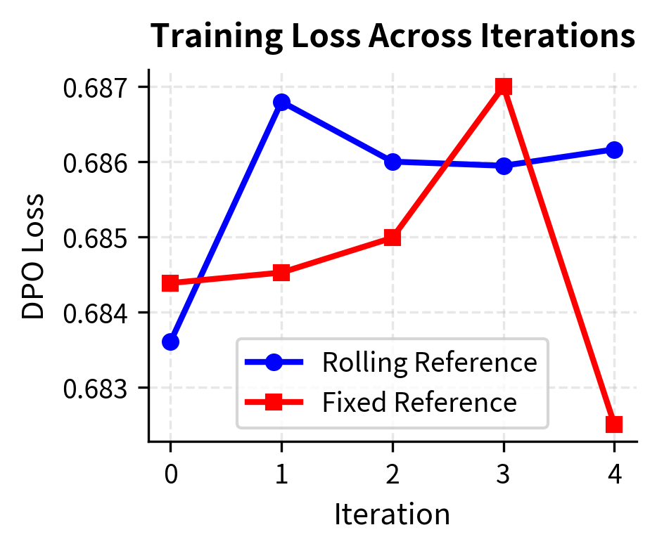
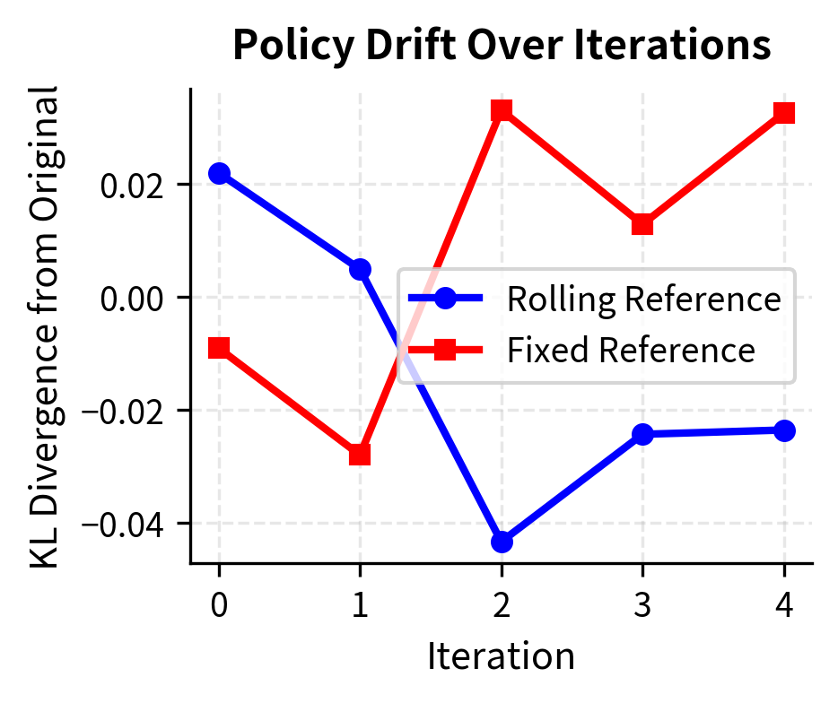
The visualization reveals an important dynamic: with a rolling reference, the KL divergence from the original model grows steadily as the policy improves through iterations. This represents the cumulative effect of iterative training. With a fixed reference, the KL growth pattern differs because the training signal always pulls toward the same anchor point.
Now let's implement a self-improvement loop using the SPIN concept.
Let's evaluate how the model's outputs change over SPIN iterations.
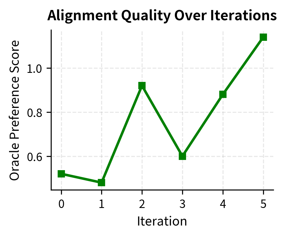
The SPIN-trained model achieves a significantly higher score, confirming that self-play fine-tuning effectively improved alignment with the oracle's preferences.
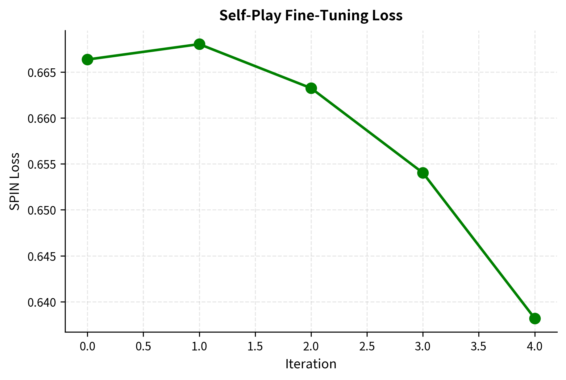
The rapid decrease in loss indicates the model is successfully optimizing the SPIN objective, learning to distinguish ground truth responses from its own generations. Finally, let's implement monitoring for alignment stability.
The metrics show the expected trade-off: as the Oracle Score improves (higher alignment), the Diversity decreases. This confirms that the model is converging onto the specific patterns rewarded by the oracle.
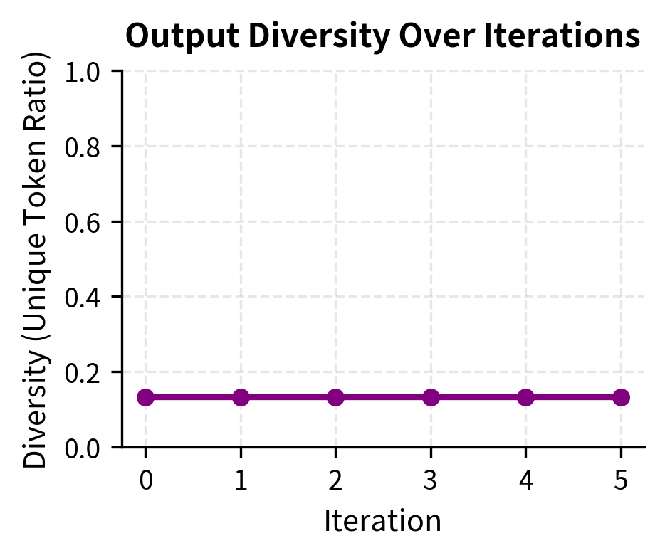
The stability metrics reveal the trade-offs inherent in iterative alignment. As the model learns to satisfy the oracle's preferences, it may sacrifice diversity, a phenomenon that warrants careful monitoring in production systems.
Key Parameters
The key parameters for the iterative alignment implementation are:
- beta: The temperature parameter controlling the strength of the KL penalty (typically 0.1). Higher values keep the model closer to the reference.
- rolling_reference: Boolean indicating whether to update the reference model at each iteration (
True) or keep it fixed (False). - num_iterations: The number of cycles of generation and training to perform.
- num_pairs: The number of response pairs generated per prompt for preference collection in each round.
Practical Considerations
Deploying iterative alignment in production requires attention to several practical issues that our simplified examples gloss over.
Iteration Frequency
How often should you iterate? Too frequent iteration (e.g., after every batch) prevents the model from fully learning from current data. Too infrequent iteration (e.g., once per quarter) allows significant distribution shift. Most practitioners find weekly to monthly iteration cycles work well, depending on the rate of model deployment and feedback collection.
Data Mixing
Rather than training exclusively on new preference data each iteration, mixing in data from previous iterations helps prevent catastrophic forgetting of earlier lessons. A common approach maintains a replay buffer of preferences from all iterations, sampling proportionally from recent and historical data.
Human-in-the-Loop Checkpoints
Even when using AI feedback for most iterations, periodic human evaluation checkpoints catch drifts that AI judges miss. These checkpoints might occur every few iterations or whenever automated metrics suggest significant behavioral changes.
Rollback Mechanisms
Sometimes iterative training goes wrong: the model develops undesirable behaviors or loses capabilities. Having clear rollback criteria and maintaining checkpoints from each iteration enables quick recovery. Define specific metrics that trigger automatic rollback: capability benchmark drops below threshold, diversity falls too low, or human evaluators flag concerning patterns.
Limitations and Impact
Iterative alignment represents a significant advance over single-shot training but introduces its own challenges. The computational cost multiplies with each iteration: you need to generate new data, potentially annotate it, and train again. For large models, this becomes expensive quickly.
The self-improvement approaches, while promising, have limits. A model cannot improve beyond what its evaluation criteria capture. If the judge model (whether human or AI) has blind spots, iterative training amplifies rather than corrects them. Constitutional AI partially addresses this with explicit principles, but those principles themselves may be incomplete or contradictory.
Perhaps most concerning is the possibility of subtle value drift. Small consistent biases in the preference signal, whether from the reward model, the AI judge, or sampling strategies, compound over iterations. After many rounds of training, the model might satisfy measured preferences while diverging from underlying human values in ways that are difficult to detect until something goes wrong.
These challenges don't diminish the importance of iterative alignment; they highlight the need for careful monitoring, diverse evaluation, and appropriate human oversight. As models become more capable, the alignment process must become more sophisticated. Single-shot training may suffice for simple tasks, but truly aligned AI systems likely require continuous, iterative refinement guided by ongoing human feedback and evaluation.
The upcoming chapters on inference optimization cover the practical machinery needed to deploy these iteratively-aligned models efficiently. Techniques like KV caching, quantization, and efficient attention make it feasible to run aligned models at scale while maintaining the quality achieved through careful iterative training.
Summary
Iterative alignment extends single-shot methods like DPO and RLHF into ongoing processes that maintain tight alignment as models and expectations evolve. Key concepts from this chapter:
- Distribution mismatch after training motivates iterative approaches: the model's outputs no longer match the distribution that generated preference data
- Iterative DPO runs multiple training rounds, with either a fixed reference (stable anchor, growing ratios) or rolling reference (stable ratios, cumulative drift)
- Online preference learning generates fresh data from the current policy, keeping training distribution matched but requiring continuous annotation
- Self-improvement through SPIN, Constitutional AI, and LLM-as-judge enables scaling beyond human annotation bottlenecks
- Stability concerns include model collapse, reward hacking accumulation, capability degradation, and subtle value drift
- Monitoring diversity, capability retention, and KL divergence from the original model helps detect problems early
- Practical deployment requires balancing iteration frequency, mixing historical data, incorporating human checkpoints, and maintaining rollback capabilities
Iterative alignment isn't a solved problem; it's an active research area with significant open questions about stability, safety, and scalability. But the core insight is clear: alignment should be a continuous process, not a one-time event.
Quiz
Ready to test your understanding? Take this quick quiz to reinforce what you've learned about iterative alignment methods.

Comments