

Learn why Chinchilla-optimal models are inefficient for deployment. Master over-training strategies and cost modeling for inference-heavy LLM systems.

This article is part of the free-to-read Language AI Handbook
Inference Scaling
The scaling laws we explored in previous chapters, from Kaplan's initial discoveries to Chinchilla's compute-optimal ratios, share a common assumption: they optimize for training efficiency. Given a fixed compute budget, how do you allocate it between model size and training data to minimize loss? This framing makes sense from a research perspective, where training costs dominate and the goal is to push capabilities forward as quickly as possible.
But production deployments face a fundamentally different optimization problem. A model is trained once, then serves inference requests continuously, potentially billions of times over its operational lifetime. When inference compute dwarfs training compute by orders of magnitude, optimizing for training efficiency can be precisely the wrong strategy.
This chapter examines how to think about scaling when inference costs matter. We'll see why the compute-optimal models from Chinchilla are actually inefficient for deployment, explore the practice of "over-training" smaller models for inference efficiency, and develop frameworks for modeling total deployment costs. The key insight is that the optimal model for training and the optimal model for serving are often very different. Understanding this distinction is essential for practical LLM deployment.
The Training-Inference Asymmetry
Consider the lifecycle of a large language model. Training is an intensive, one-time process that might consume millions of GPU-hours over several weeks. Once complete, the model enters production, where it handles inference requests: generating text, answering questions, or processing documents. This serving phase can extend for months or years.
The asymmetry becomes stark when you examine actual compute consumption. To appreciate why this matters so much: think about what happens each time you query a language model. Every single token the model generates requires a forward pass through the entire network. Billions of parameters are activated, multiplied, and transformed. When a model serves millions of users, each generating hundreds or thousands of tokens per interaction, these individual operations compound into astronomical compute requirements.
To quantify this rigorously, we can calculate the total FLOPs consumed during inference and compare it to training cost. A training run might use FLOPs (roughly what it takes to train a 70B parameter model on 2 trillion tokens). If that model then serves 1 billion inference requests, each generating an average of 500 tokens, the total inference compute is:
where:
- : total compute required for all inference requests over the model's deployment
- : number of inference requests served
- : average number of output tokens generated per request
- : floating-point operations required to generate one token
This formula captures a fundamental insight about deployment economics: inference cost grows linearly with each of these three factors. More users, longer responses, or larger models all increase the compute burden proportionally. The multiplicative structure means that even modest increases in any factor can dramatically shift the overall compute balance.
For a forward pass through an -parameter model, inference requires approximately FLOPs per token (one multiply-add per parameter). This figure deserves attention because it reveals something important about transformer efficiency: every parameter in your model must be activated for every token you generate. There's no shortcut, no way to skip over unused portions of the network. The full weight matrix participates in every prediction. For our 70B model:
This is about 7% of training compute. This is significant, but training still dominates in this scenario. At this scale, the traditional wisdom of optimizing for training efficiency still holds. However, if the model serves 100 billion requests:
Now inference compute exceeds training compute by a factor of 7. This crossover point, where inference begins to dominate, is the key threshold that determines whether training-optimal or inference-optimal strategies should guide model selection. Understanding where your deployment falls relative to this threshold is crucial for making economically sound decisions about model architecture and training strategy.
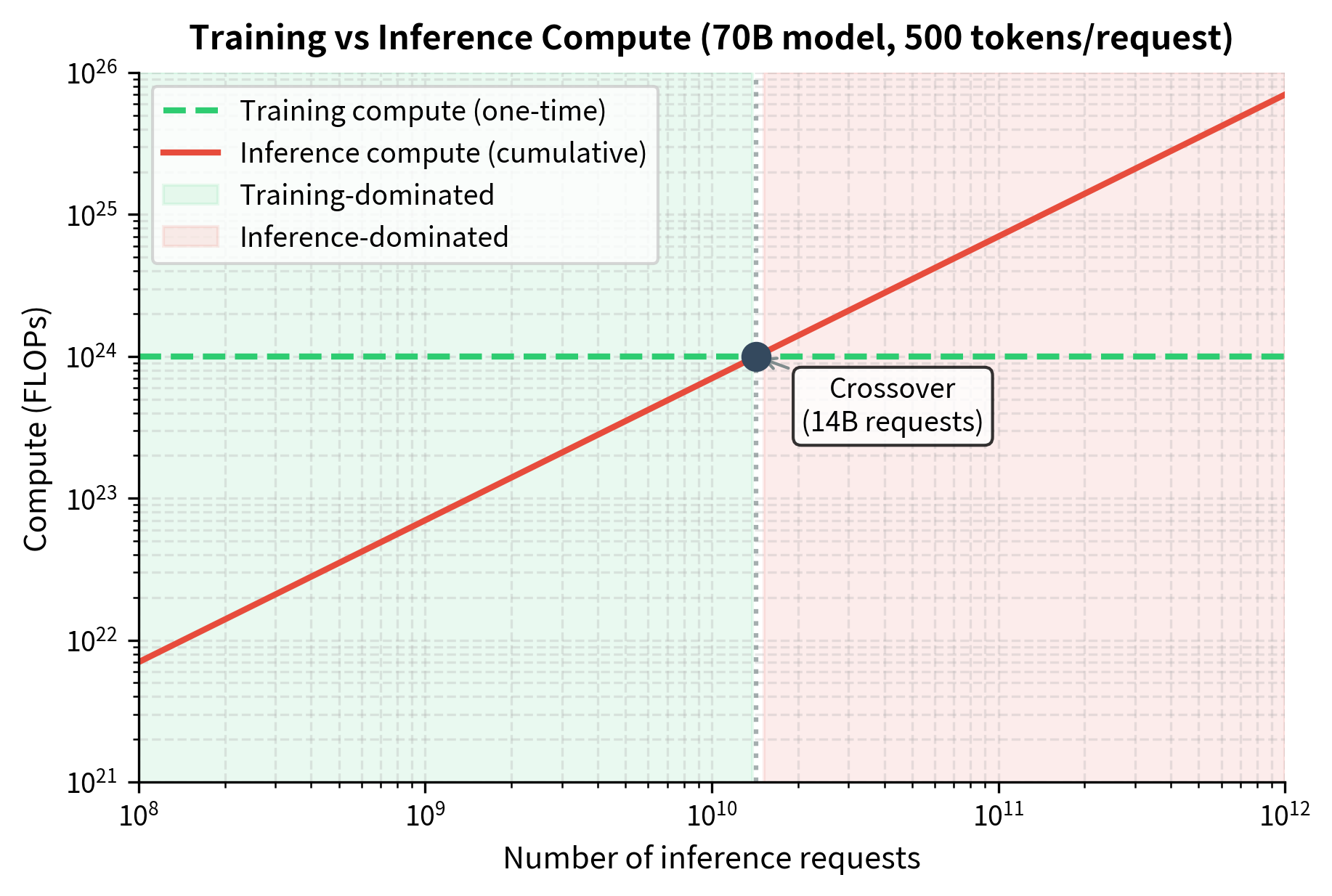
For the most widely deployed models serving trillions of requests, inference can consume 100× or more compute than training. Consider a model like GPT-4 or Claude serving millions of users worldwide, each engaging in multiple conversations per day over the course of years. The cumulative inference load dwarfs even the most expensive training runs.
This asymmetry fundamentally changes the optimization calculus. When training dominates, you want the most capable model you can train within your compute budget. When inference dominates, you want the smallest model that achieves acceptable quality, even if training it costs more per unit of capability gained. This shift in perspective—from training-centric to deployment-centric optimization—represents one of the most important practical insights in applied machine learning.
Why Chinchilla is Training-Optimal, Not Deployment-Optimal
Recall from the Chinchilla scaling laws chapter that compute-optimal training allocates compute roughly equally between model size and data, following the relationship where is tokens trained and is parameters. This minimizes training FLOPs to reach a target loss. The elegance of this ratio—roughly 20 tokens per parameter—emerged from careful empirical study and provides a clear recipe for efficient training.
But the Chinchilla framework optimizes for a specific objective: minimizing the compute required to achieve the lowest possible loss during training. It treats training as the end goal rather than as a means to an end. When we recognize that the true objective is efficient deployment, not efficient training, the optimal strategy shifts dramatically.
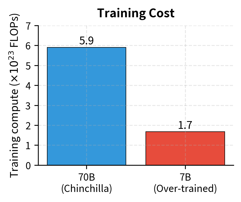
Consider two models trained to the same final loss:
Model A (Chinchilla-optimal):
- 70B parameters
- 1.4T tokens
- Training compute: FLOPs
The approximation comes from the fact that each training token requires a forward pass ( operations) plus a backward pass (approximately operations for computing gradients), totaling operations per token across tokens. This 6-to-1 ratio between training and inference compute per token is another fundamental constant worth internalizing. It explains why training is so much more expensive than inference on a per-token basis, but also why inference costs accumulate so quickly when serving many users.
where:
- : number of model parameters
- : number of training tokens
- : total FLOPs, accounting for forward pass (2 operations per parameter per token) plus backward pass (roughly 4 operations per parameter per token)
Model B (Over-trained):
- 7B parameters
- 4T tokens (requires longer training to match Model A's loss)
- Training compute: FLOPs
Model B actually uses less training compute to reach the same loss. How can this be? The key is that Chinchilla optimality assumes you're pushing to the frontier of what's achievable at a given compute level. If you're willing to accept a specific target loss rather than minimizing loss for fixed compute, smaller models trained longer can sometimes be more efficient even for training.
This counterintuitive result arises because Chinchilla optimality answers a different question than the one we're asking. Chinchilla asks: "Given a fixed compute budget, how do I get the lowest possible loss?" The deployment question asks: "Given a target quality level, how do I minimize total cost over the model's lifetime?" These are fundamentally different optimization problems with different optimal solutions.
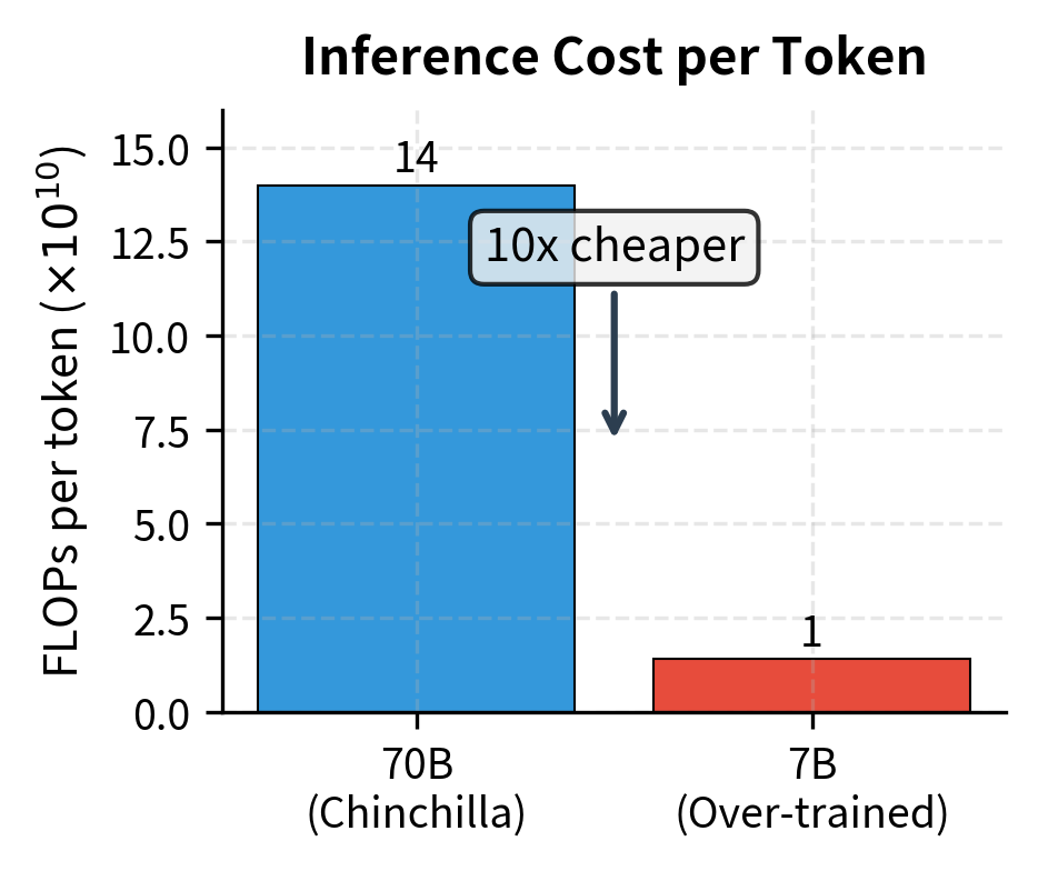
The real advantage of smaller models emerges at inference time. Model A requires FLOPs per output token, while Model B requires FLOPs per token—10× fewer inference FLOPs for equivalent quality.
This 10× reduction in per-token cost compounds with every inference request. If both models serve a billion requests, Model B saves approximately FLOPs per token generated. This compute savings translates directly to reduced electricity bills, fewer GPUs required, and lower operational costs.
For high-volume deployments, this 10× inference efficiency can translate to massive cost savings that dwarf any training cost difference.
Over-Training for Deployment Efficiency
"Over-training" refers to training a model on more tokens than Chinchilla optimality would suggest. The term is slightly misleading, as it's only "over" training relative to compute-optimal. It's exactly the right amount of training for inference-optimal deployment. Think of it not as excessive training but as investing additional training compute to reduce inference costs later.
The LLaMA Philosophy
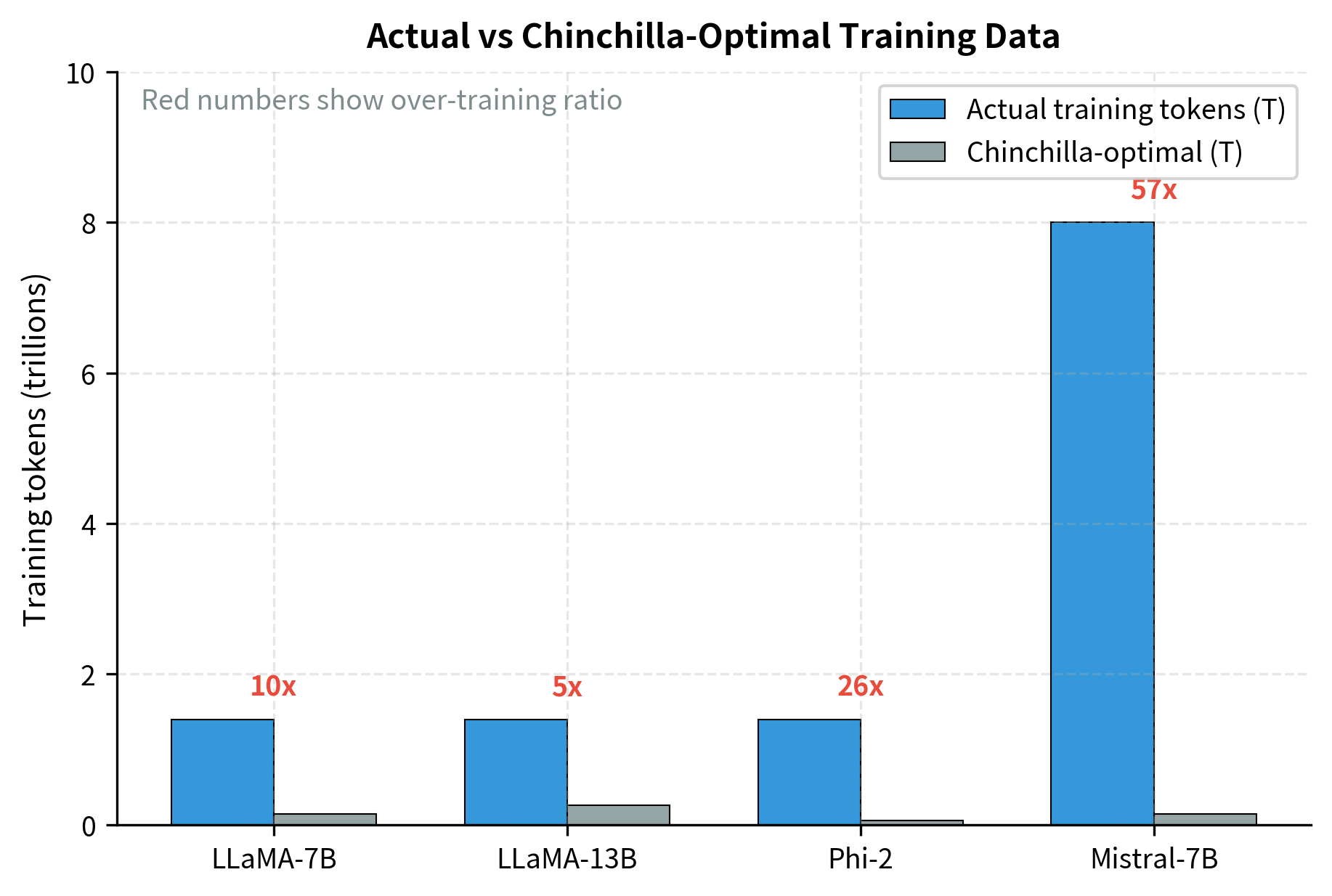
The LLaMA model family explicitly adopted this philosophy. The LLaMA paper states: "We only consider the performance of the resulting model, not the training compute budget." They trained 7B, 13B, 33B, and 65B parameter models on up to 1.4 trillion tokens. This is far more than Chinchilla ratios would suggest for the smaller models.
This statement represents a philosophical break from the Chinchilla paradigm. Rather than asking how to minimize training compute, Meta's researchers asked how to maximize the value delivered per inference FLOP. This reframing led to models that were "inefficient" to train but were much more efficient to deploy.
For the 7B model, Chinchilla optimality would suggest around 140B tokens. Training on 1.4T tokens represents 10× "over-training." This extra training compute is an investment that pays dividends at inference time through reduced per-token cost. Every additional training token helps the smaller model close the capability gap with larger alternatives, making it suitable for tasks that would otherwise require a more expensive model.
The Over-Training Ratio
We can quantify over-training with a simple ratio that captures how far a model departs from Chinchilla-optimal training:
where:
- : the number of tokens the model is actually trained on
- : the Chinchilla-optimal number of tokens for a model of size
- : the number of model parameters
- : the Chinchilla approximation that optimal training uses roughly 20 tokens per parameter
This ratio provides a simple metric for characterizing how inference-optimized a model's training regime is. A ratio of 1 means the model was trained according to Chinchilla-optimal principles. Ratios greater than 1 indicate over-training for inference efficiency, with higher values representing more aggressive investment in training compute to reduce inference costs.
The table below shows typical over-training ratios for inference-optimized models:
| Model | Parameters | Tokens | Chinchilla Optimal | Over-training Ratio |
|---|---|---|---|---|
| LLaMA-7B | 7B | 1.4T | 140B | 10× |
| LLaMA-13B | 13B | 1.4T | 260B | 5.4× |
| Mistral-7B | 7B | ~8T | 140B | ~57× |
| Phi-2 | 2.7B | 1.4T | 54B | 26× |
Modern inference-optimized models routinely use over-training ratios of 10× to 50× or more. The trend toward higher ratios reflects growing recognition that inference costs dominate for production systems. Mistral's 57× over-training ratio on their 7B model demonstrates how far this philosophy has been pushed. They invested roughly 57 times more training compute than Chinchilla would recommend. They bet that the resulting inference efficiency would more than compensate.
When Over-Training Pays Off
Over-training makes economic sense when total inference compute exceeds the extra training compute required. Let's formalize this break-even analysis, which provides the mathematical foundation for deployment decisions.
Suppose you have two options:
- Option 1: Train a large model on tokens (Chinchilla-optimal)
- Option 2: Train a smaller model on tokens to match Option 1's loss
The additional training cost for Option 2 is:
where:
- : the difference in training compute between the two options
- : parameter counts for Option 1 (larger) and Option 2 (smaller) respectively
- : training tokens for Option 1 and Option 2 respectively
This difference can be positive or negative depending on the specific model sizes and training durations. If the smaller model requires enough additional training to offset the reduced parameter count, will be positive, representing an upfront investment that must be recouped through inference savings.
The inference savings per token generated are:
Here, represents the FLOPs saved per output token by using the smaller model (since each forward pass requires FLOPs per token).
This quantity is always positive when , meaning smaller models always save inference compute regardless of how they were trained. The magnitude of these savings grows linearly with the difference in model sizes—a 63B parameter reduction saves 63 billion fewer multiply-add operations per token.
Over-training pays off when total inference tokens satisfies:
This break-even analysis determines whether the inference savings justify the training investment. The inequality has a clear interpretation: the left side represents cumulative inference savings over the model's deployment, while the right side represents the upfront training cost differential. When expected inference volume exceeds the break-even point, the smaller over-trained model becomes the economically rational choice.
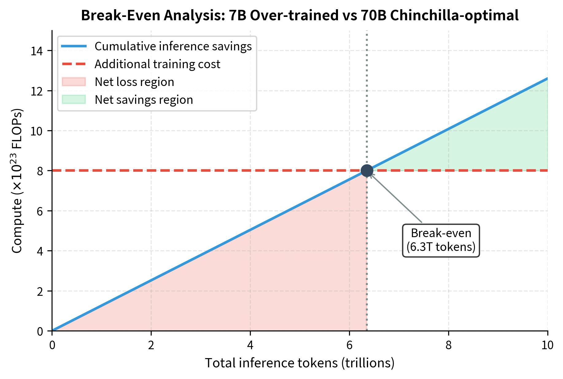
Worked Example: Break-Even Analysis
Let's work through a concrete comparison between a 70B Chinchilla-optimal model and a 7B over-trained model, both achieving similar loss. This example illustrates the practical magnitude of the cost differences and helps build intuition for deployment decisions.
Option 1: 70B model, 1.4T tokens
- Training: FLOPs
- Inference: FLOPs/token
Option 2: 7B model, 4T tokens (assume this matches 70B model's loss)
- Training: FLOPs
- Inference: FLOPs/token
In this case, Option 2 actually costs less to train. This can happen when targeting a specific loss level rather than frontier performance. The inference savings are:
Every inference token saves FLOPs, and there's no training penalty—only savings. This represents a best-case scenario where the over-trained model wins on both training and inference efficiency, highlighting how the conventional wisdom about "larger models being better" can be misleading for deployment contexts.
Even when over-training does cost more, break-even typically occurs at modest inference volumes. If the 7B model required FLOPs to train (an additional FLOPs over the 70B option), the break-even would be:
At 500 tokens per request, that's about 12.6 billion inference requests, easily exceeded by any widely-deployed model. To put this in perspective, a popular API serving just 10,000 users, each making 10 requests per day, would reach this break-even point in roughly 3.4 years. For consumer-scale deployments with millions of users, break-even occurs within days or weeks of launch.
Inference-Optimal Model Selection
Given expected inference demand, we can determine the optimal model size directly. This requires understanding how loss scales with both model size and training data, and then reformulating the optimization problem to account for total lifecycle costs rather than just training costs.
The Inference-Optimal Scaling Law
Building on the Chinchilla loss function from earlier chapters:
where:
- : the model's loss as a function of size and training data
- : the number of model parameters
- : the number of training tokens
- : empirically fitted scaling coefficients
- : empirically fitted exponents (typically around 0.34 and 0.28)
- : the irreducible error floor representing the entropy of natural language
This functional form captures two distinct pathways to reducing loss: adding more parameters (the first term) or training on more data (the second term). The irreducible error floor represents the fundamental uncertainty in language—even a perfect model cannot predict with certainty what word comes next in human text. Understanding this structure is essential for reasoning about the trade-offs between model size and training duration.
We can reformulate the optimization problem for inference-dominant scenarios. Rather than minimizing loss for a fixed training budget (the Chinchilla approach), we want to minimize loss for a fixed total budget that includes both training and expected inference. This reformulation shifts the optimization target from training efficiency to deployment efficiency.
The total compute over the model's lifecycle is:
where:
- : total compute over the model's entire lifecycle
- : training compute (approximately 6 FLOPs per parameter per token)
- : total inference compute (2 FLOPs per parameter per token generated)
- : expected total tokens generated during the model's deployment
This formulation captures the key insight: training cost is paid once, but inference cost accumulates with every token generated. The training term depends on both and (model size times data), while the inference term depends on and (model size times usage). This asymmetric structure—where model size appears in both terms but data appears only in training—is what drives the preference for smaller models in high-inference scenarios.
To minimize loss subject to a total compute budget, we take derivatives and solve. The resulting optimal allocation shifts toward smaller models as expected inference volume increases:
where:
- : the optimal model size (number of parameters) for the given deployment scenario
- : the total compute budget available across training and inference
- : expected total tokens to be generated during deployment
- : positive exponents derived from the scaling law parameters and . The exact values depend on the specific scaling law coefficients, but typical values yield and
The negative exponent on is the key result: it shows mathematically that optimal model size decreases as expected inference volume increases. This relationship emerges directly from the calculus of constrained optimization. When inference tokens grow, the cost of each parameter (which must be activated for every token) grows proportionally, pushing the optimum toward fewer parameters.
The intuition is clear: as inference demand grows, the optimal model size shrinks because each parameter incurs a cost at every inference, while training cost is amortized. A parameter that costs billions of FLOPs to train well might seem expensive, but if that parameter is then used trillions of times at inference, the training cost becomes negligible compared to the cumulative inference burden.
Practical Model Size Selection
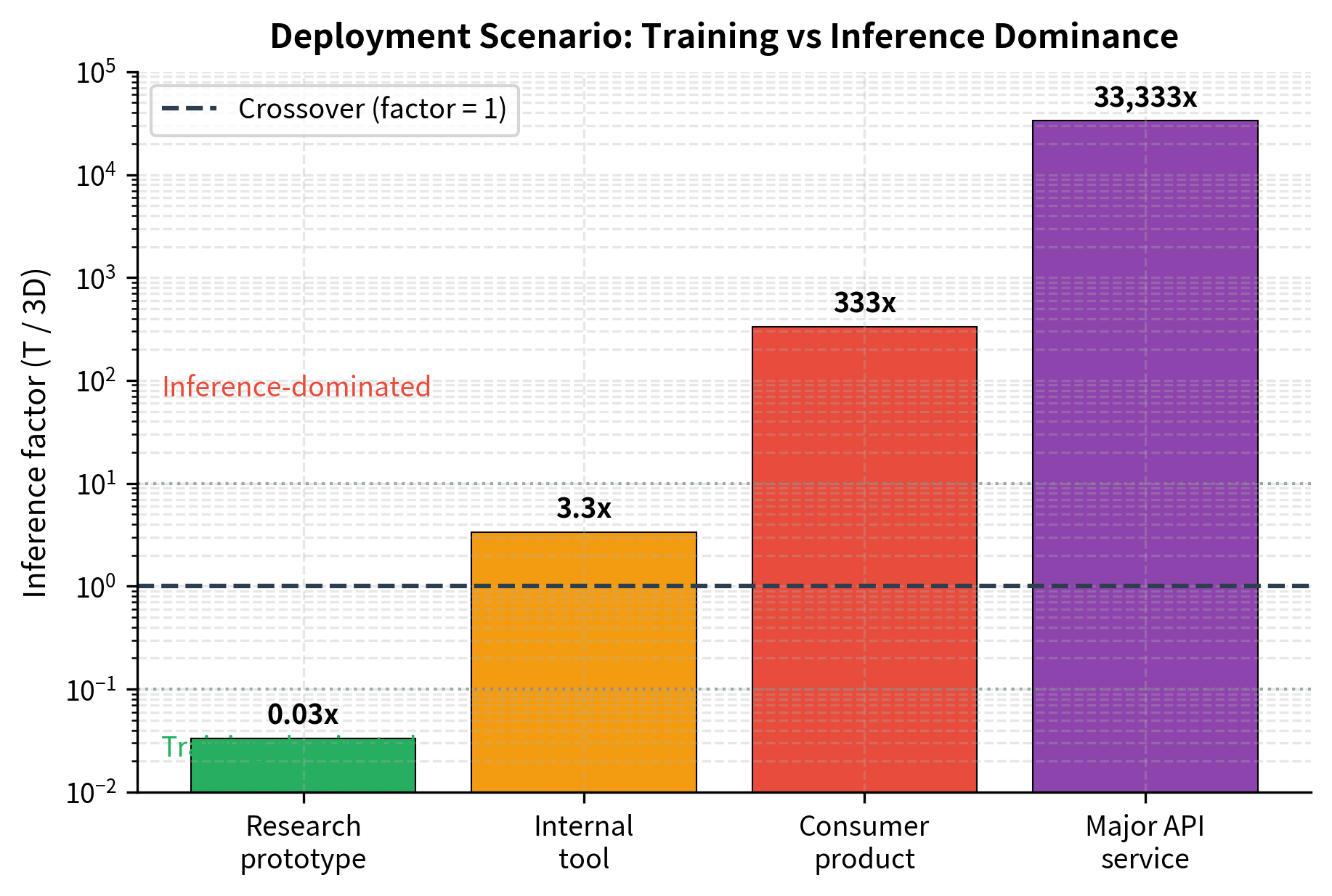
For deployment planning, a simplified heuristic helps guide model selection. If you expect to generate inference tokens over the model's lifetime, compare the inference compute to training compute:
where:
- : total inference tokens expected over the model's deployment lifetime
- : number of tokens used for training
- : model parameters (which cancel out in the simplification)
Notice that cancels out. The inference factor depends only on the ratio of inference tokens to training tokens. This cancellation is mathematically elegant and practically useful because you can evaluate whether inference will dominate without even knowing the model size. When this factor exceeds 1, inference compute dominates. The larger this factor, the more aggressively you should favor smaller, over-trained models.
The inference factor provides a simple decision rule. Values below 1 indicate training-dominated scenarios where Chinchilla-optimal sizing remains appropriate. Values above 1 signal that inference costs will outweigh training costs, justifying investment in smaller, more heavily trained models. Values above 10 suggest aggressive over-training is warranted. Values above 100 indicate that inference efficiency should be the primary design consideration.
The output reveals how dramatically the optimal strategy shifts based on expected usage. The research prototype shows an inference factor of just 0.03×, meaning training compute still dominates, so Chinchilla-optimal sizing remains appropriate. But as we move to consumer products (333×) and major API services (33,333×), inference compute overwhelms training by orders of magnitude. At these scales, every parameter becomes a recurring cost multiplied across trillions of tokens, making aggressive over-training the only economically rational choice. A research prototype with limited deployment can safely follow Chinchilla scaling, while a consumer-facing API should aggressively over-train smaller models.
Deployment Cost Modeling
Real deployment decisions involve more than FLOP counting. Hardware costs, memory constraints, latency requirements, and energy consumption all factor into the total cost of ownership. Moving from theoretical compute analysis to practical cost modeling requires understanding how FLOPs translate to dollars and how hardware constraints shape achievable throughput.
Components of Deployment Cost
A comprehensive cost model includes:
- Hardware amortization: The cost of training and inference hardware amortized over useful life
- Compute costs: Electricity and cooling, proportional to FLOPs executed
- Memory costs: Larger models require more expensive hardware configurations
- Latency penalties: Slower inference may reduce user engagement or transaction value
- Opportunity costs: Resources committed to one model can't serve others
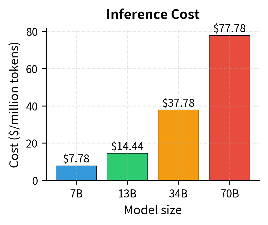
The Cost-Per-Token Model
For a concrete cost analysis, we model the cost to generate one inference token. This simple economic model divides fixed hourly costs by throughput: fewer tokens per hour means each token must bear a larger share of the infrastructure cost:
This formula reveals the fundamental economic structure of inference: you're paying for GPU time, and the question is how many tokens you can squeeze out of each hour of that expensive hardware. Higher throughput means lower per-token costs, which is why inference optimization focuses so heavily on maximizing tokens per second.
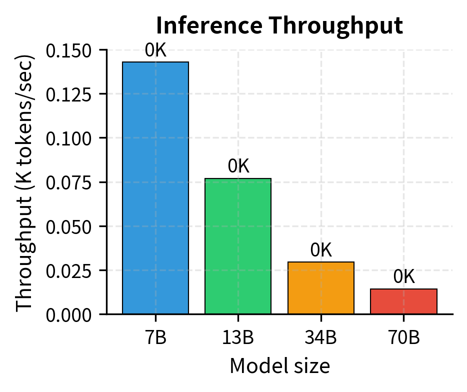
Tokens per hour depends on model throughput, which is constrained by either compute or memory bandwidth:
where:
- : tokens generated per second
- : the GPU's floating-point operations per second
- : FLOPs required per token (two operations per parameter for the forward pass)
- : bytes per second the GPU can read from memory
- : memory footprint per parameter (e.g., 2 bytes for FP16)
The minimum captures a fundamental hardware constraint: generation speed is limited by whichever resource (compute or memory bandwidth) is exhausted first. This bottleneck analysis is crucial for understanding real-world inference performance.
The first term () represents the theoretical maximum if compute were the only constraint, dividing total available operations by operations needed per token. This would be the limit if weights could be loaded from memory instantaneously.
The second term captures the memory bottleneck: each token generation requires loading all model weights from memory, so throughput cannot exceed memory bandwidth divided by model size. The autoregressive generation process must stream the entire weight matrix through the GPU's memory bus for every single token produced.
For large models, memory bandwidth typically dominates, making smaller models even more advantageous than pure FLOP analysis suggests. Modern GPUs have tremendous compute capacity but relatively limited memory bandwidth. An A100 can perform 312 trillion floating-point operations per second but can only move 2 trillion bytes per second from memory. For large models, the weights cannot be loaded fast enough to keep the compute units busy.
Implementing a Cost Calculator
The following code implements a deployment cost model incorporating these factors:
The analysis shows that inference costs scale superlinearly with model size—a 10× larger model costs more than 10× per token due to memory bandwidth constraints. The 7B model achieves roughly 143,000 tokens per second with a total cost around $0.028 per million tokens, while the 70B model drops to about 14,000 tokens per second at approximately $0.28 per million tokens. Notably, all models in this analysis are memory-bound rather than compute-bound, meaning the limiting factor is how fast weights can be loaded from GPU memory—not the GPU's raw computational capacity. This memory bottleneck is why smaller models gain such dramatic throughput advantages. This reinforces the value of smaller, over-trained models for production deployments.
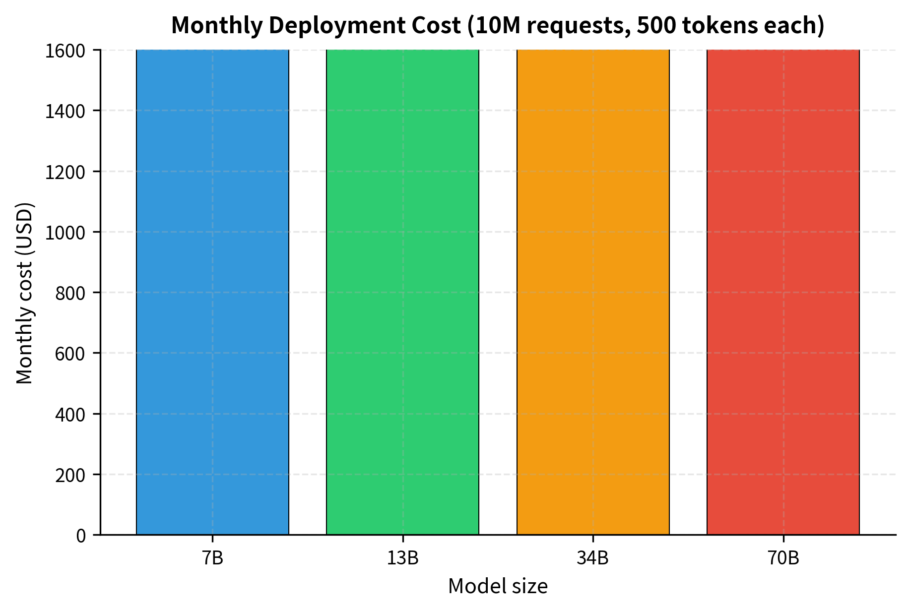
Monthly Deployment Cost Estimation
For capacity planning, we can project monthly costs based on expected request volume:
The cost differential between model sizes is substantial. For this scenario of 10 million requests generating 5 billion tokens monthly, the 7B model costs approximately $140 per month while the 70B model costs around $1,400, a 10× difference. Both require only a single GPU for continuous coverage at this volume, but the 7B model leaves far more headroom for traffic spikes. Choosing a 7B over-trained model instead of a 70B compute-optimal model can reduce monthly costs by 90% or more while maintaining comparable quality for many use cases.
Trade-offs and Practical Considerations
Inference scaling decisions involve more than raw compute costs. Several practical factors influence the optimal model size.
Quality Degradation Limits
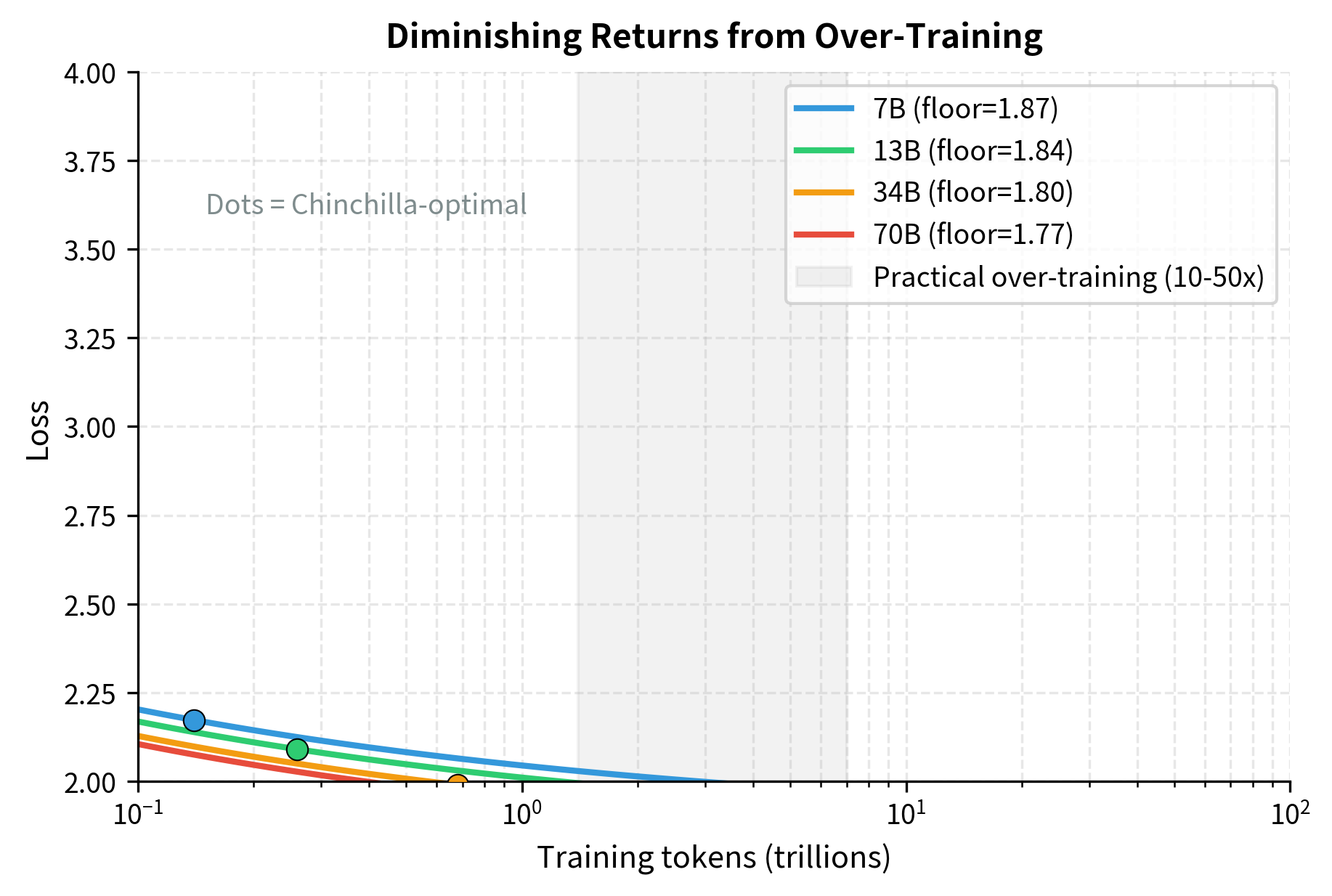
Over-training has diminishing returns. As you train a smaller model on more data, it eventually hits capacity limits, and additional training provides minimal benefit. The loss curve for a fixed model size approaches an asymptote:
This equation shows the fundamental capacity limit of any fixed-size model: no amount of additional training data can push the loss below the floor set by model size and the irreducible entropy of language.
where:
- : the model's loss as a function of parameters and training data
- : empirically fitted scaling coefficient for model capacity
- : model size raised to the scaling exponent (typically )
- : irreducible error floor (entropy of natural language)
- : the limit as training data approaches infinity
This limit shows what happens when a fixed-size model is trained on infinite data: the data-dependent term vanishes, leaving only the model capacity term and the irreducible error floor . The model capacity term represents limitations inherent to the architecture. A 7B model simply cannot represent certain complex patterns that a 70B model can capture. These architectural constraints set hard limits on how much over-training can compensate for fewer parameters.
Research suggests that models can be productively over-trained by roughly 10-50× before returns diminish significantly. Beyond that, you're paying for training compute that yields minimal quality improvement.
Task-Specific Considerations
Different tasks have different sensitivity to model size. Smaller models may:
- Struggle with complex reasoning chains
- Have weaker few-shot learning compared to larger models
- Show degraded performance on rare or specialized domains
- Exhibit less robustness to adversarial or unusual inputs
For applications requiring these capabilities, accepting higher inference costs may be necessary. The next chapter on predicting model performance will provide frameworks for estimating these task-specific capabilities.
Memory Constraints
Larger models require proportionally more GPU memory. A 70B FP16 model needs 140GB just for weights, exceeding single-GPU capacity and requiring model parallelism. This introduces:
- Higher latency from cross-GPU communication
- Reduced batch efficiency
- More complex deployment infrastructure
Smaller models that fit on a single GPU often achieve better effective throughput despite needing to load parameters for every token.
Batching Efficiency
Production inference servers batch multiple requests together, amortizing the cost of loading model weights across many tokens. Batching efficiency improves with model size to a point, but larger models have smaller maximum batch sizes due to memory constraints.
The optimal batch size trades off:
- Throughput (higher batches = better GPU utilization)
- Latency (larger batches = longer queue times)
- Memory (each request consumes activation memory)
Key Parameters
The key parameters for inference-optimal deployment are:
- Over-training ratio: The factor by which actual training tokens exceed Chinchilla-optimal tokens (). Ratios of 10-50× are common for inference-optimized models.
- Inference factor: The ratio of expected inference tokens to training tokens (). When this exceeds 1, inference costs dominate and smaller models become preferable.
- Memory bandwidth: Often the limiting factor for large model inference throughput, not raw compute capacity.
- Bytes per parameter: Determines model memory footprint (2 bytes for FP16, 1 byte for INT8). Smaller values enable larger batch sizes and better throughput.
Limitations and Impact
Inference scaling analysis provides valuable guidance but has important limitations. The cost models presented here use simplified assumptions: they assume that throughput is constrained by either compute or memory bandwidth in isolation. Real systems exhibit more complex behavior where both constraints interact, speculative decoding changes the compute-per-token relationship, and quantization techniques (which we'll cover in later chapters) can significantly shift the efficiency landscape.
The "tokens generated" framing also obscures the distinction between the prefill phase (processing the input prompt) and the decode phase (generating output tokens). Prefill is compute-bound and can be batched efficiently, while decode is typically memory-bound. Models serving long prompts with short outputs have different cost profiles than those generating lengthy responses from brief prompts.
Despite these limitations, inference scaling has profoundly influenced how the field develops and deploys models. The LLaMA model family demonstrated that inference-optimized training could produce models competitive with much larger alternatives. This work catalyzed the open-source LLM ecosystem. Organizations now routinely train smaller models on more data than Chinchilla would suggest, accepting higher training costs to achieve better deployment economics.
This shift has also influenced architecture design. Techniques like grouped-query attention, which we covered in the LLaMA components chapter, reduce memory bandwidth requirements and improve inference efficiency. The focus on inference has accelerated research into quantization, speculative decoding, and other techniques that reduce the effective cost per token.
Summary
This chapter explored how scaling laws change when inference costs dominate training costs, as they do for any widely-deployed model:
-
The training-inference asymmetry means that models are trained once but may serve trillions of inference requests. When inference compute exceeds training compute, optimizing for training efficiency becomes counterproductive.
-
Chinchilla is training-optimal, not deployment-optimal. The compute-optimal ratios minimize training cost to reach a given loss, but don't account for the per-token inference cost that accumulates over deployment.
-
Over-training refers to training smaller models on more data than Chinchilla ratios suggest. This invests additional training compute to achieve lower inference costs—a trade-off that pays off rapidly for high-volume deployments.
-
The break-even analysis determines when over-training becomes economical, specifically when the total inference savings exceed the additional training investment. For production systems, break-even often occurs at modest request volumes.
-
Deployment cost modeling must account for hardware constraints, memory bandwidth limitations, energy costs, and the superlinear relationship between model size and inference cost.
-
Practical model selection depends on expected inference volume, quality requirements, latency constraints, and infrastructure capabilities. The optimal choice balances these factors rather than optimizing any single metric.
The inference scaling perspective completes our picture of how to allocate compute across the model development lifecycle. Combined with the training-focused scaling laws from earlier chapters, you now have frameworks for optimizing both phases of the compute budget. The next chapter extends these ideas to predict how model performance varies across different capabilities and benchmarks.
Quiz
Ready to test your understanding? Take this quick quiz to reinforce what you've learned about inference scaling and deployment optimization.

Comments