Data-Constrained Scaling: Training LLMs Beyond the Data Wall

The Chinchilla scaling laws from our previous chapter offer a straightforward recipe: to train a compute-optimal model, scale parameters and training tokens in roughly equal proportion. A 70 billion parameter model should see approximately 1.4 trillion tokens. But this prescription contains a hidden assumption that becomes increasingly problematic as models grow larger: it assumes we have unlimited unique training data.

In practice, we don't. The internet, despite its vastness, contains a finite amount of high-quality text. As the AI community trains ever-larger models, we're approaching what researchers call the "data wall": the point where compute-optimal training would require more unique tokens than exist. This chapter examines what happens when data becomes the binding constraint, how repeated data affects model quality, and strategies for stretching limited data resources.

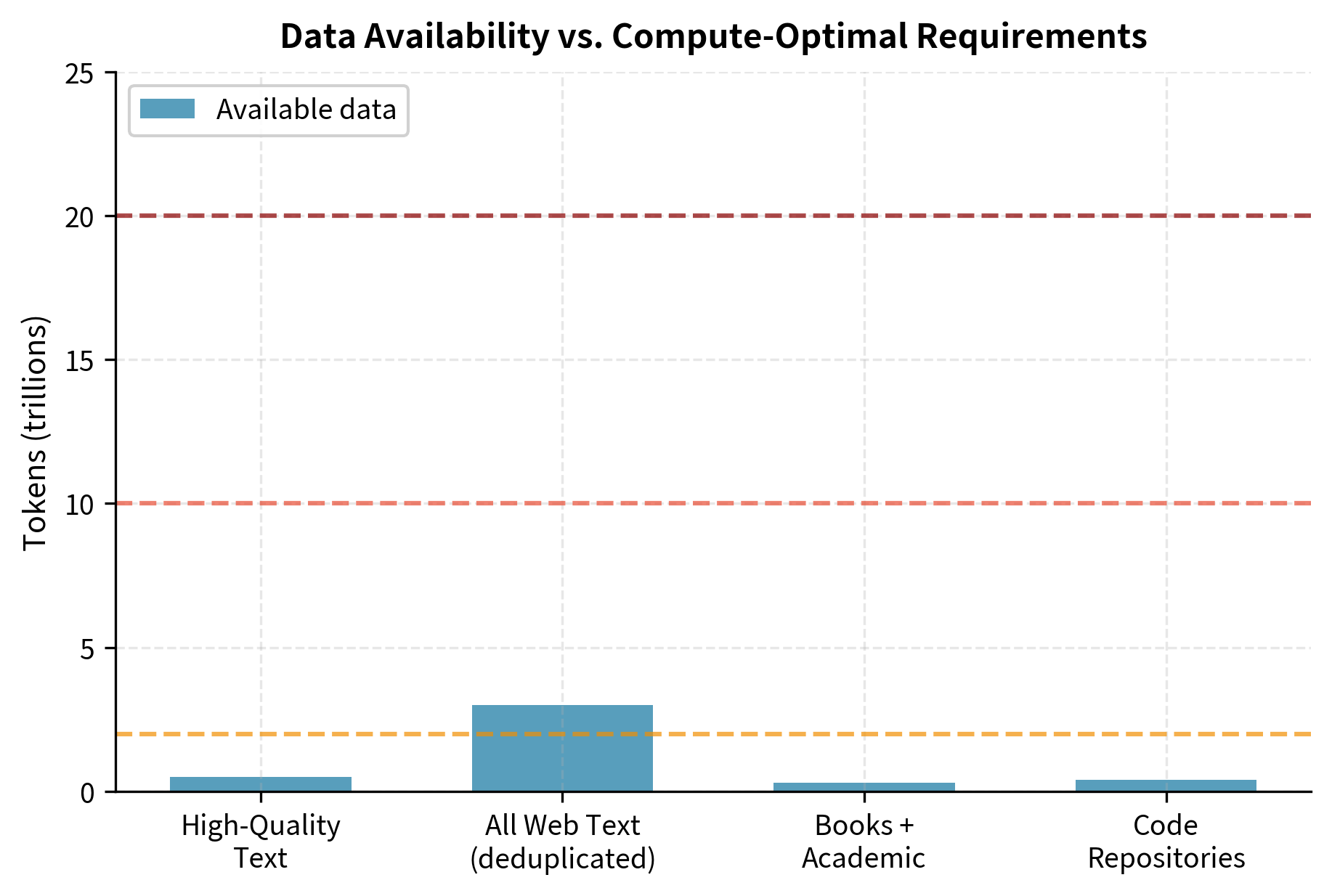
To understand the data constraint, consider the scale of modern training corpora. The Pile, a widely-used open dataset, contains approximately 825 GB of text, yielding roughly 300 billion tokens. Common Crawl, the largest web scrape, provides about 3 trillion tokens after deduplication and filtering. These numbers sound enormous until you apply Chinchilla-optimal ratios.

A 1 trillion parameter model, following Chinchilla guidelines, would need approximately 20 trillion training tokens. That is roughly seven times the entire deduplicated Common Crawl. A 10 trillion parameter model would require 200 trillion tokens, far exceeding all text ever produced by humanity.

Villalobos et al. (2022) systematically estimated when various data sources would be exhausted. Their analysis revealed a sobering timeline:

• High-quality text (books, academic papers, curated web content): Exhausted by 2026-2028 at current scaling rates
• All web text: Exhausted by 2030-2032
• Multimodal data (images, video): Provides more runway but with different utility

This isn't merely a theoretical concern. Training runs for GPT-4 and similar models already approach or exceed the high-quality data ceiling. The question is no longer whether we'll hit the data wall, but how to train effectively when we do.

When unique data runs out, the natural response is to repeat existing data, training on the same examples multiple times across different epochs. But repetition is not free. Each additional pass through the same data yields diminishing returns, and excessive repetition can actively harm model quality. To understand why, consider what a neural network learns during training and how that learning changes when the network has already seen an example.

Muennighoff et al. (2023) conducted the first systematic study of data repetition in language model scaling, training models ranging from 25 million to 8.7 billion parameters with varying degrees of repetition. Their findings confirmed what practitioners suspected:

Repeated data is worth less than unique data. A model trained on 100 billion unique tokens significantly outperforms one trained on 25 billion tokens repeated four times, even though both see the same total token count. The gap widens as repetition increases. This result challenges a naive view where tokens are interchangeable units of learning signal. Instead, the novelty of information matters significantly.

Returns diminish rapidly. The first repetition (seeing data twice) captures perhaps 70-80% of the value of unique data. The fourth repetition might capture only 30-40%. Beyond 8-16 repetitions, additional passes contribute almost nothing to final performance. This pattern reflects how gradient-based learning works: early passes make large updates that capture the broad structure of the data, while later passes can only make small refinements to already-learned patterns.

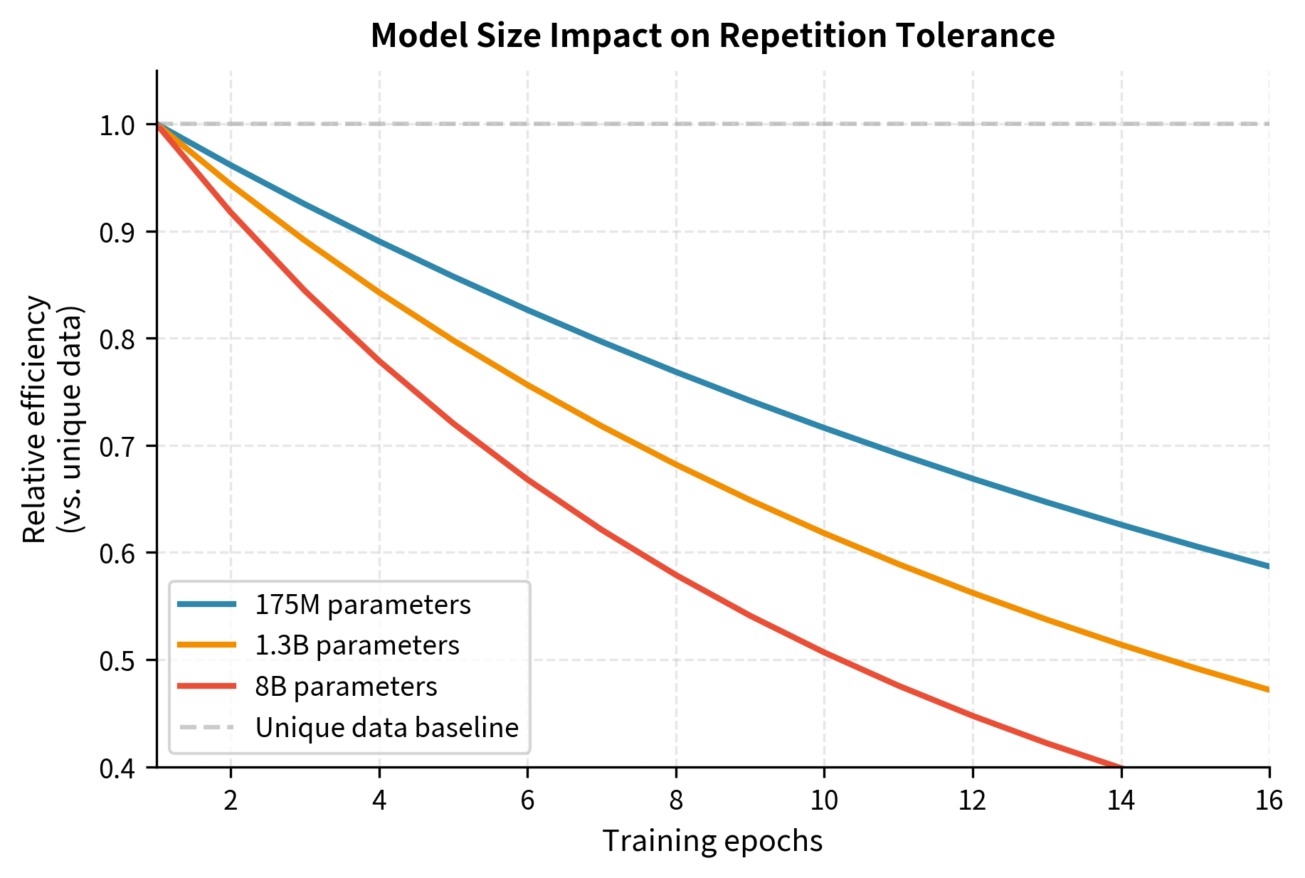
Larger models suffer more from repetition. A 175 million parameter model tolerates 16 epochs with modest degradation. An 8 billion parameter model shows measurable harm after just 4 epochs. This makes intuitive sense: larger models have more capacity to memorize, and they extract more information per pass, leaving less to learn on subsequent passes. A small model might need multiple exposures to fully capture a complex pattern, while a large model grasps it on the first pass, making subsequent passes redundant.

Researchers formalize repetition effects through what we might call an "epoch penalty": a multiplier that discounts the effective value of repeated tokens. If unique tokens have a value of 1.0, the $n$-th repetition of a token has value $f(n) < 1$.

Before diving into the mathematical formulation, let's build intuition for what we're trying to capture. Imagine reading a textbook chapter for the first time. You absorb enormous amounts of new information. Reading it a second time still helps: you catch details you missed, reinforce your understanding, and make new connections. By the fifth reading, you're mostly confirming what you already know. By the twentieth reading, you're gaining almost nothing. The mathematical framework below captures exactly this diminishing pattern.

The functional form of this penalty follows an exponential saturation pattern (despite common references to "power law" behavior in scaling contexts, the repetition penalty specifically uses exponential decay). Let $D$ be the number of unique tokens and $R$ be the number of epochs (repetitions). The effective number of tokens $D_{\text{eff}}$ is not simply $D \times R$, but rather:

where:

• $D_{\text{eff}}$: the effective number of training tokens after accounting for repetition penalty
• $D$: the number of unique tokens in the dataset
• $g(R)$: a function that captures the diminishing returns from repetition, mapping epochs to an effective multiplier

The key insight here is that $g(R)$ grows more slowly than $R$ itself. If repetition had no penalty, we would have $g(R) = R$, and effective tokens would simply equal total tokens processed. The entire purpose of introducing $g(R)$ is to quantify how much value we lose to repetition.

Muennighoff et al. found that $g(R)$ is well-approximated by:

where:

• $R$: the number of epochs (times the data is repeated)
• $\alpha$: a decay constant controlling how quickly returns diminish (empirically fitted to approximately 0.1)
• $e^{-\alpha R}$: exponential decay term that approaches zero as repetitions increase
• $e^{-\alpha}$: the single-epoch decay factor, used to normalize the function so that $g(1) = 1$

Let's unpack why this particular mathematical form makes sense. The numerator $1 - e^{-\alpha R}$ is a classic saturation curve. It starts at zero when $R=0$ and approaches 1 as $R$ grows large. This captures the intuition that no matter how many times you repeat the data, you can only extract a finite amount of information from it. The denominator $1 - e^{-\alpha}$ is simply a normalization constant that ensures $g(1) = 1$, meaning one pass through the data has full value.

The parameter $\alpha$ controls the rate of saturation. When $\alpha$ is small (as the empirically fitted value of 0.1 suggests), the saturation happens slowly—you can repeat data many times before hitting severe diminishing returns. If $\alpha$ were larger, returns would diminish more quickly, and even modest repetition would waste computational resources.

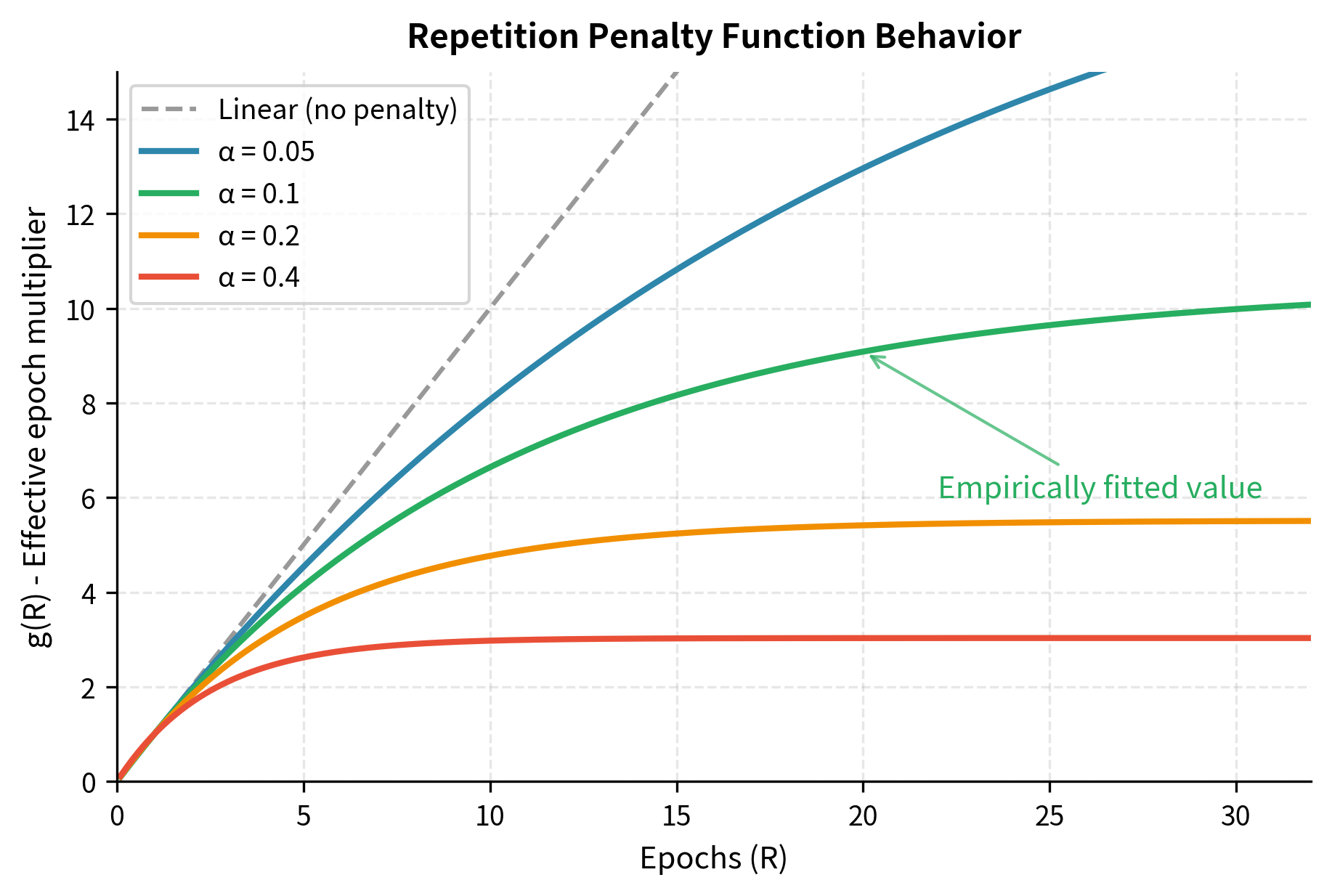
This functional form has two useful properties. First, $g(1) = 1$, meaning there is no penalty for seeing data once—a single pass through the data contributes its full value. Second, $g(R)$ asymptotes to a finite limit as $R \to \infty$, meaning there is a maximum effective dataset size regardless of how many times you repeat the data. Specifically, as $R$ grows without bound, the exponential term $e^{-\alpha R}$ vanishes, and $g(R)$ approaches $1/(1 - e^{-\alpha})$. For $\alpha = 0.1$, this asymptotic limit is approximately 10.5, meaning that infinite repetition of your data is equivalent to having roughly 10.5 times as much unique data. This asymptotic behavior captures the intuition that you cannot extract infinite value from finite data through repetition alone.

Incorporating repetition effects into the Chinchilla framework requires modifying the loss function. This modification represents an important conceptual shift. We move from treating all tokens as equivalent to recognizing that the information content of tokens depends on whether we've seen them before.

Recall that the basic Chinchilla loss takes the form:

where:

• $L(N, D)$: the expected loss (cross-entropy) for a model with $N$ parameters trained on $D$ tokens
• $N$: the number of model parameters
• $D$: the number of training tokens
• $A, B$: empirically fitted scaling coefficients
• $\alpha, \beta$: exponents controlling how loss decreases with scale (approximately 0.34 and 0.28 respectively)
• $E$: irreducible loss representing the entropy of natural language (the theoretical minimum loss even with infinite model size and data)

The formula captures a fundamental tradeoff: the first term $A/N^\alpha$ represents the capacity limitation of the model (reducible by adding more parameters), while the second term $B/D^\beta$ represents the data limitation (reducible by adding more training tokens). The irreducible loss $E$ represents patterns in language that are inherently unpredictable. Understanding this decomposition is essential because data-constrained scaling fundamentally alters how we can address the data limitation term.

Think of the first term as "how much the model could learn but lacks the capacity to store," and the second term as "how much the model could store but has not yet seen." In the standard Chinchilla framework, we can freely trade off between these by adjusting model size and data quantity. But when data is constrained, the second term becomes partially frozen, and we can only reduce it so much before running out of unique information.

When data is repeated, we replace $D$ with $D_{\text{eff}}$:

where:

• $L(N, D, R)$: the expected loss for a model with $N$ parameters trained on $D$ unique tokens for $R$ epochs
• $D_{\text{eff}}$: the effective token count after accounting for repetition penalty, computed as $D \times g(R)$
• $N, A, B, \alpha, \beta, E$: retain their meanings from the standard Chinchilla loss above

This substitution has a subtle but profound effect on the loss landscape. In the original formulation, increasing $D$ always improves loss (with diminishing returns governed by $\beta$). In the modified formulation, increasing epochs $R$ improves $D_{\text{eff}}$, but the improvement saturates. Eventually, the marginal gain in effective data from additional epochs becomes negligible, while the computational cost continues to grow linearly.

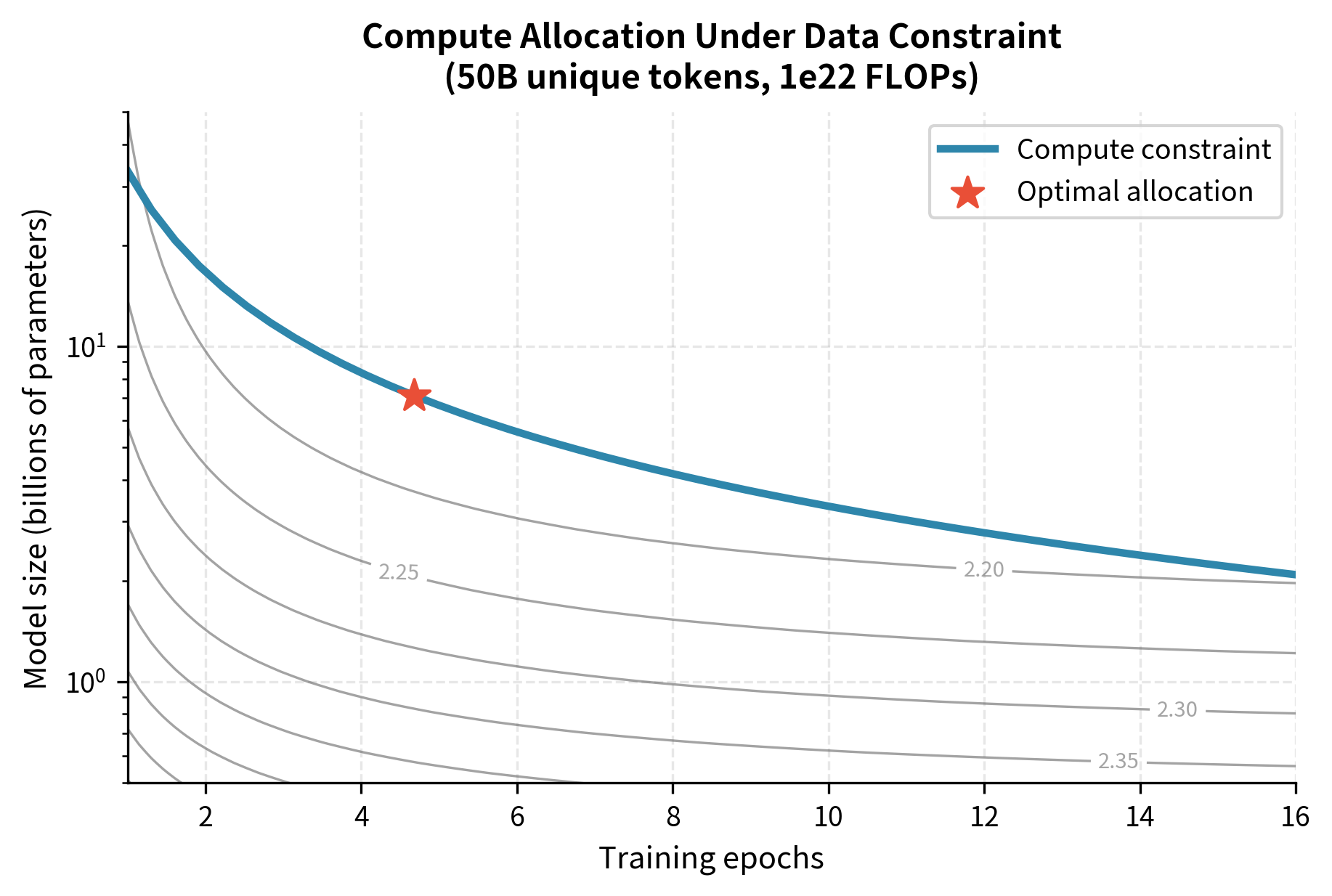
This modification has significant implications for compute-optimal training. Under the original Chinchilla law, doubling compute should roughly double both $N$ and $D$. Under data-constrained scaling, once $D$ is fixed at the available unique data, additional compute should go primarily toward larger models with more repetitions—but with awareness that the marginal value of additional training decreases. The key tradeoff becomes: given fixed unique data $D$, how should we allocate compute between model size $N$ and number of epochs $R$? The answer depends on solving for the minimum of $L(N, D, R)$ subject to the compute constraint $C = 6NRD$ (approximately 6 FLOPs per parameter per token per epoch).

This optimization problem no longer has the elegant closed-form solution of the original Chinchilla analysis. Instead, practitioners must numerically search over possible allocations, as we demonstrate in the code implementation section below.

Since repetition has diminishing returns, how should practitioners allocate resources when data is limited? The answer depends on available compute, dataset size, and target model size.

Consider a fixed compute budget $C$ and dataset size $D$. You can train a smaller model for more epochs or a larger model for fewer epochs. The optimal choice balances three factors:

Model capacity determines how much information can be extracted per example. Larger models learn more from each pass.

Epoch diminishing returns means additional passes yield less. The penalty is steeper for larger models.

Compute cost scales with both model size and tokens processed. Larger models cost more per token.

The optimal strategy is to train the largest model that can complete a "reasonable" number of epochs within your compute budget. "Reasonable" depends on the repetition penalty: Muennighoff et al. suggest that performance degrades unacceptably beyond approximately 4 epochs for large models.

Based on empirical studies, practitioners should consider several guidelines when operating under data constraints:

• When unique data is sufficient for compute-optimal training, use it without repetition. This is the ideal scenario where Chinchilla ratios apply directly.

• When moderate data limitation exists (requiring 2-4 epochs), proceed with training but expect approximately 10-20% higher loss than the compute-optimal equivalent with unlimited data.

• When severe data limitation exists (requiring 8+ epochs), consider these alternatives before extensive repetition: reduce model size to require fewer tokens, invest compute in data quality improvement and deduplication, or explore synthetic data augmentation.

An underappreciated finding from scaling research is that data quality and quantity are not simply additive. Smaller amounts of high-quality data often outperform larger amounts of lower-quality data, and this advantage compounds with repetition.

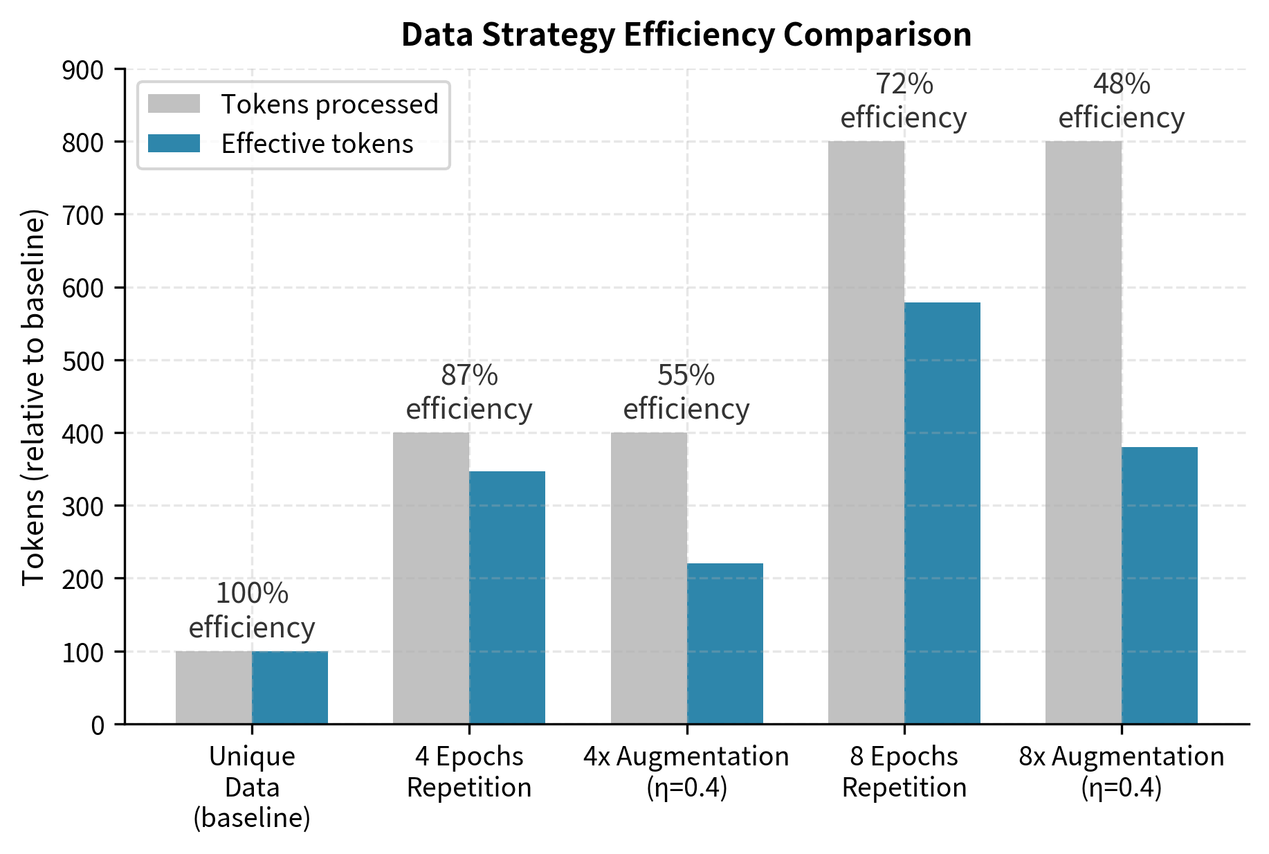
Consider a choice between 50 billion tokens of carefully curated text (books, Wikipedia, academic papers) and 200 billion tokens of raw web crawl. Training on the curated data with 4 repetitions (200 billion total tokens) typically outperforms single-epoch training on raw crawl, despite the latter having four times the unique examples. The curated data benefits from higher information density per token and cleaner signal for learning linguistic patterns.

This suggests that when facing data constraints, investment in data curation may yield better returns than acquiring more raw data.

Traditional NLP relied heavily on data augmentation, transforming existing examples to create new training instances. Techniques like back-translation, synonym substitution, and random deletion could multiply dataset size by 10× or more. How do these techniques interact with scaling?

The most common augmentation techniques for language modeling include:

• Back-translation: Translates text to another language and back, creating paraphrases that preserve meaning but vary in surface form. A sentence like "The cat sat on the mat" might become "The feline rested upon the rug" after round-trip translation through French.

• Synonym substitution: Replaces words with synonyms using a thesaurus or word embeddings. This creates lexical variation while maintaining semantic content.

• Random operations: Include deletion, insertion, and swap operations that add noise while preserving most structure. Deleting 10% of words or swapping adjacent words creates varied examples.

• Paraphrase generation: Uses trained paraphrase models to rewrite sentences with different syntactic structures.

Augmentation provides less value at scale than researchers initially hoped. Several studies found that augmented data behaves more like repeated data than unique data. This makes sense. Augmentations preserve the underlying semantic content while varying surface features. A model quickly learns to see through superficial variations, treating augmented examples as near-duplicates.

To understand this phenomenon more deeply, consider what a language model actually learns. At a superficial level, it learns associations between word sequences. But at a deeper level, it learns semantic relationships, factual knowledge, and reasoning patterns. Augmentation techniques typically preserve the deeper content while only varying the surface form. A model sophisticated enough to benefit from massive scale is also sophisticated enough to recognize that "The cat sat on the mat" and "The feline rested upon the rug" convey the same information, even if the tokens differ.

The effective repetition factor for augmented data is approximately 0.3-0.5 compared to unique data. More formally, if we denote the augmentation effectiveness as $\eta \approx 0.3-0.5$, then generating $k$ augmented variants yields effective data:

where:

• $D$: the number of original unique tokens
• $k$: the number of variants per example (original + augmentations)
• $\eta$: the augmentation effectiveness factor (how much value each augmented example provides relative to a unique example)

Let's trace through the logic of this formula. We start with $D$ original tokens, which contribute their full value. We then add $k-1$ augmented variants (since $k$ includes the original). Each augmented variant contributes only $\eta$ times the value of a unique example. So our total effective data is the original $D$ plus the discounted value of the augmentations: $D + D \cdot \eta \cdot (k-1) = D \cdot (1 + \eta \cdot (k-1))$.

An augmentation that produces 5 variants of each example ($k=5$) with $\eta=0.4$ might yield effective data equivalent to $D \cdot (1 + 0.4 \cdot 4) = 2.6D$, approximately 2.6 repetitions worth rather than 5 unique examples. This represents a significant gap: you have done five times the computational work of processing unique data but gained less than three times the effective training signal.

This doesn't mean augmentation is useless—it's often better than raw repetition. But it's not a solution to the data wall. Transforming 100 billion tokens into 1 trillion augmented tokens does not yield performance equivalent to 1 trillion unique tokens.

Augmentation shows the strongest benefits in two scenarios:

• Low-resource settings: Settings where base data is severely limited (less than 1 billion tokens) benefit substantially from augmentation. The model has not fully memorized the training set, so variations provide genuine learning signal.

• Domain-specific fine-tuning: Scenarios where acquiring more in-domain data is impractical can leverage augmentation. If you have only 10,000 medical documents, augmentation can help prevent overfitting during fine-tuning.

For large-scale pretraining where data is measured in trillions of tokens, augmentation provides marginal value compared to its computational cost.

If augmented data provides limited value, what about entirely synthetic data? Modern language models can generate coherent, novel text. Could we use model-generated data to train the next generation of models?

This question has generated intense research interest, with results that are simultaneously promising and concerning.

The appeal is clear. Language models can generate unlimited text. If synthetic data were as valuable as natural data, the data wall would dissolve. Training would be constrained only by compute, and we could generate as much data as needed.

Reality is more nuanced. Synthetic data quality depends critically on the generator model, the generation strategy, and how synthetic data is mixed with natural data.

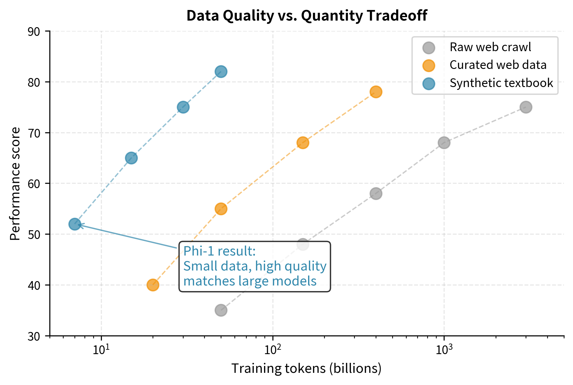
The most successful synthetic data approaches emphasize quality over quantity. Microsoft's Phi-1 model demonstrated this dramatically. A 1.3 billion parameter model trained primarily on synthetic "textbook-quality" data matched or exceeded models ten times larger trained on web crawl.

The key insight was using GPT-4 to generate not just any text, but specifically educational content designed for learning. The synthetic data consisted of:

• Textbook chapters explaining programming concepts step-by-step
• Exercises with varying difficulty levels
• Synthetic code with clear, well-documented examples

This curated synthetic data proved more valuable token-for-token than natural web data. One token of synthetic textbook was worth approximately ten tokens of random web crawl for learning coding abilities.

How synthetic data is generated matters enormously. Simply prompting a model to "generate text about X" yields bland, repetitive content. Effective strategies include:

• Curriculum-aware generation: Produces data spanning difficulty levels. Easy examples establish foundations; hard examples push capabilities.

• Diverse seed prompting: Uses varied prompts to ensure coverage across topics, styles, and formats. A thousand different prompt templates yield more diverse output than one template run a thousand times.

• Self-instruct: Has models generate instructions and completions, creating task-diverse training data. This approach powers much of modern instruction tuning.

• Verification filtering: Generates many candidates and filters to high-quality examples. For code, this might mean keeping only examples that compile and pass tests. For math, keeping only solutions that reach correct answers.

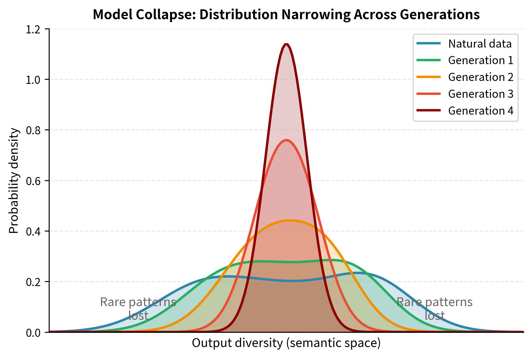
Synthetic data also carries risks. Shumailov et al. (2023) identified "model collapse," a phenomenon where models trained on synthetic data from previous model generations progressively degrade.

The mechanism is subtle but important. Each model generation slightly shifts the data distribution toward higher-probability outputs and away from the tails. Rare but important patterns (unusual words, unconventional syntax, domain-specific terminology) become rarer in synthetic data than in natural data.

When model $G_1$ generates training data for model $G_2$, the training distribution shifts. When $G_2$ generates data for $G_3$, the shift compounds. After several generations, the distribution has collapsed toward a narrow subset of high-probability outputs, and models lose capability on anything outside this narrow core.

The implications are concerning. If the internet becomes dominated by AI-generated content, future models trained on web crawls might suffer progressive capability loss.

Several strategies help prevent model collapse:

• Mixing synthetic with natural data: Maintains anchoring to the true distribution. Successful approaches typically use 50-80% natural data even when synthetic data is available.

• Freshness filtering: Preferentially uses synthetic data that is novel relative to the training set. If a generated example is too similar to existing data, discard it.

• Diversity objectives: Explicitly optimize for varied outputs during generation, using techniques like diverse beam search or temperature annealing.

• Watermarking: Tags AI-generated content, allowing future training pipelines to identify and appropriately weight synthetic data.

We can simulate data repetition effects to build intuition about how repetition degrades effective data value. The code that follows implements the mathematical framework we developed above, allowing us to see concretely how the repetition penalty affects training decisions.

This function implements the repetition penalty formula. The alpha parameter controls how quickly returns diminish. Notice how the implementation directly translates the mathematical formula we derived earlier: the exponential saturation curve $g(R)$ modulates the raw token count to produce an effective count that grows more slowly than the naive expectation.

The efficiency column reveals the harsh reality of repetition. By 4 epochs, each token is worth only about 85% of its naive value. By 16 epochs, efficiency drops to roughly 63%—you're processing 16× the tokens but getting only about 10× the effective training signal. This quantifies why practitioners should carefully consider whether additional epochs are worth the computational cost. The gap between naive expectation and effective value represents pure computational waste—FLOPs spent on redundant learning signal.

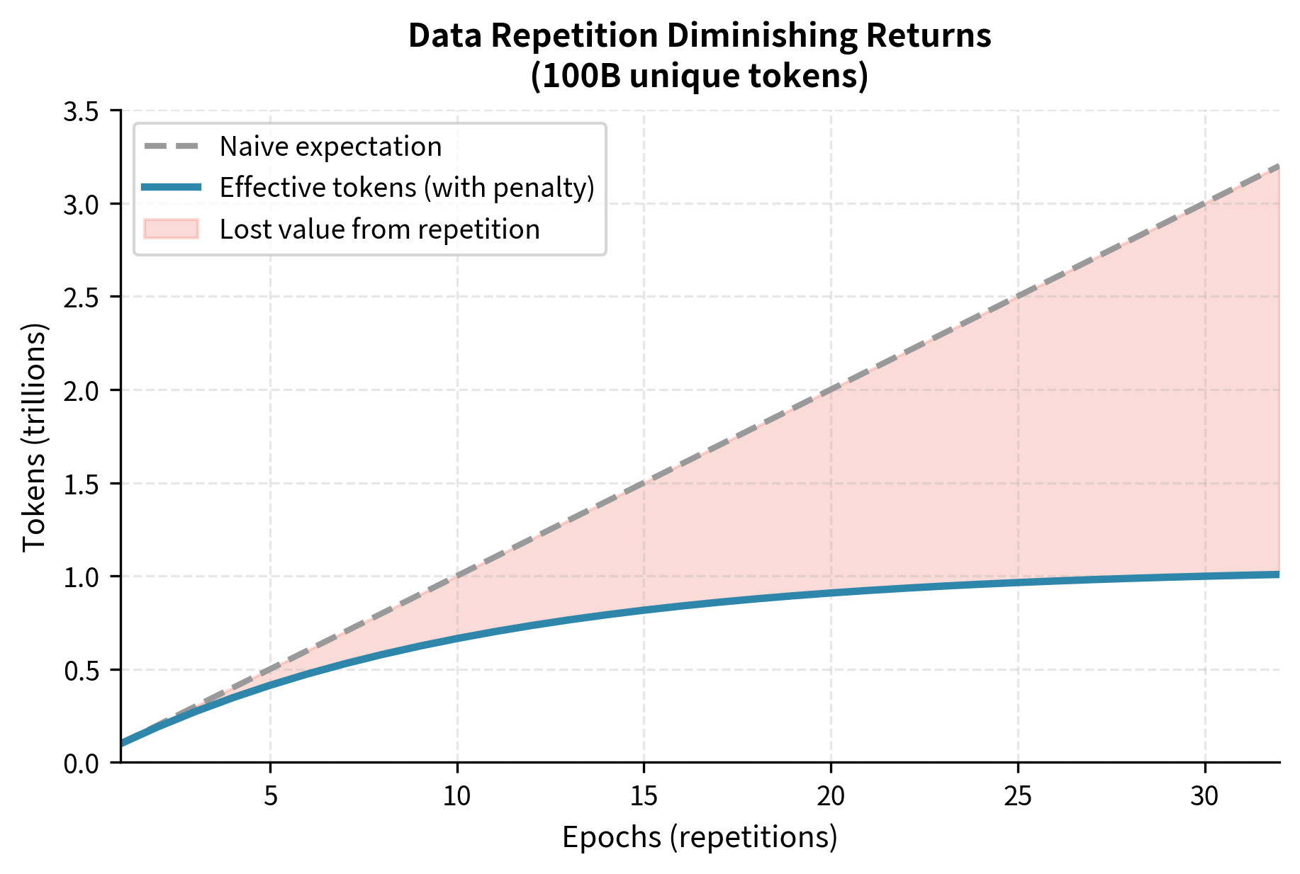
The growing gap between naive expectation and effective tokens represents the fundamental cost of data repetition. The shaded region in the figure—growing wider with each additional epoch—represents computational resources that produce no corresponding improvement in model capability. Now let's examine how this affects optimal model sizing and compare scenarios with different data availability.

The find_optimal_allocation function performs the key optimization we discussed earlier. Given a fixed compute budget and data constraint, it searches over possible epoch counts to find the configuration that minimizes final loss. For each epoch count, it calculates the corresponding model size (since compute = 6 × parameters × tokens processed), computes the effective token count using our repetition penalty formula, and evaluates the resulting loss. This brute-force search replaces the elegant closed-form solutions available under unconstrained Chinchilla scaling.

We compare three scenarios representing different levels of data availability, from abundant (1 trillion tokens) to scarce (10 billion tokens). This comparison illuminates how the same compute budget produces dramatically different outcomes depending on data availability—a crucial insight for organizations planning training runs.

The results illustrate how data availability shapes optimal training strategy. With abundant data (1T tokens), the model can grow large while maintaining single-epoch training. As data becomes scarcer, the optimizer accepts more repetition epochs but the effective training signal shrinks, resulting in higher final loss despite using the same compute budget. The loss increase from 2.296 to 2.502 when moving from abundant to scarce data represents a substantial capability gap—equivalent to what might take 10× more compute to overcome through scaling alone. Notice also how the optimal model size shifts: with scarce data, the optimizer chooses a much larger model (174.8B vs 27.8B) that trains for more epochs, extracting maximum value from each precious unique token.

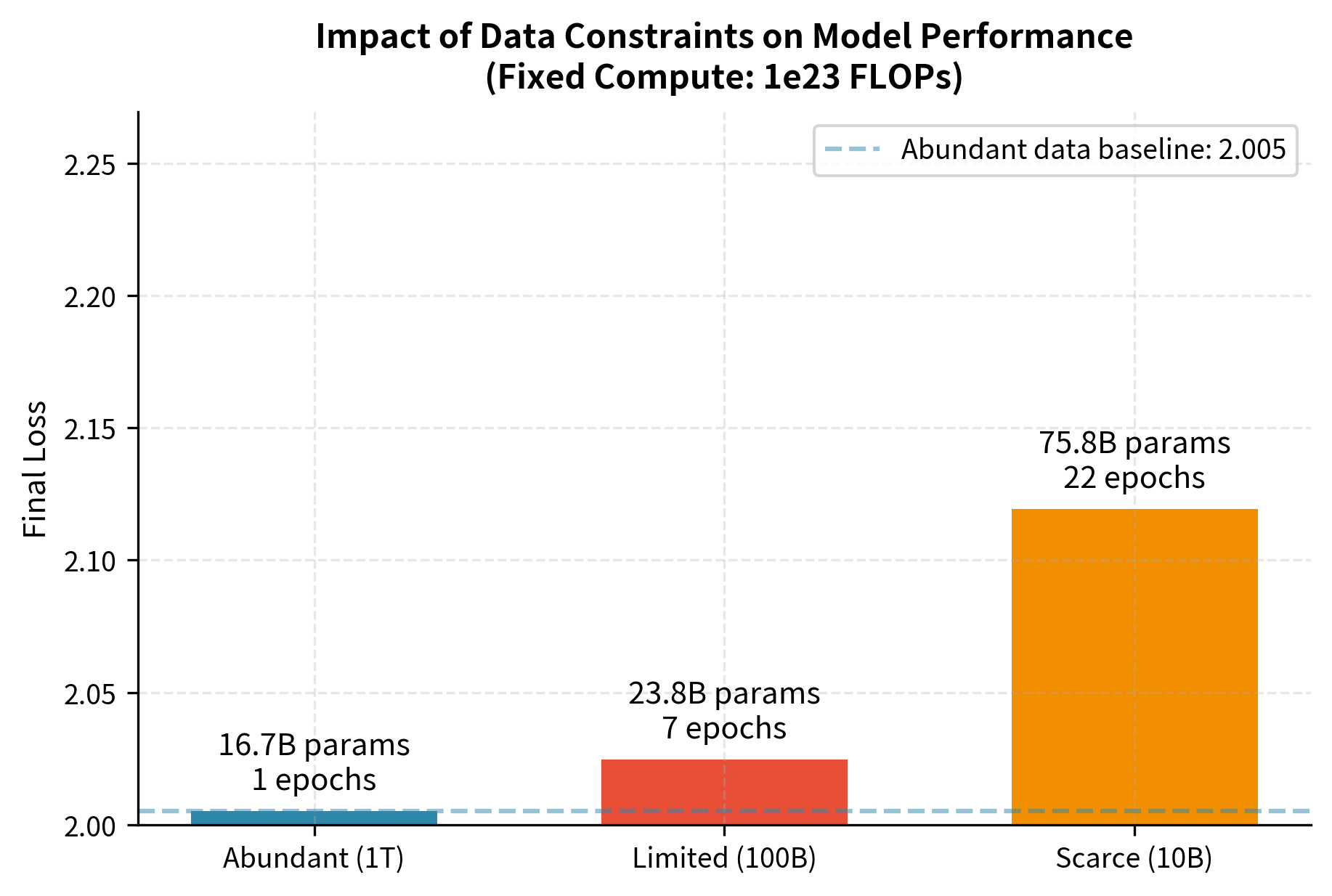
The visualization makes clear that data scarcity exacts a significant toll even with optimal compute allocation. Moving from abundant to limited data increases loss by about 0.1, while moving to scarce data adds another 0.1. These differences may seem small but translate to meaningful capability gaps in practice. The annotations on each bar reveal the hidden story: as data becomes scarcer, the optimizer dramatically increases model size while accepting more epochs, but the repetition penalty means this strategy can only partially compensate for the missing unique data.

The key parameters for data-constrained scaling are:

• alpha (repetition decay): Controls how quickly the value of repeated data diminishes. Empirically fitted to approximately 0.1. Lower values mean slower decay and more tolerance for repetition.
• epochs: Number of times the training data is repeated. Beyond 4-8 epochs, returns diminish sharply for large models.
• unique_tokens: The amount of deduplicated, unique training data available. This is the hard constraint that cannot be circumvented through repetition.
• A, B (scaling coefficients): Empirically fitted constants in the Chinchilla loss formula that determine the relative importance of model size vs. data.
• alpha, beta (scaling exponents): Control how loss decreases with scale, approximately 0.34 and 0.28 respectively.

The data-constrained scaling framework reveals several important truths about the current trajectory of language model development. Understanding these limitations is essential for both researchers and practitioners.

The most important limitation is that no amount of repetition, augmentation, or clever optimization can substitute for genuine data diversity. The scaling laws we've discussed treat tokens as fungible units, but real learning requires exposure to varied concepts, phrasings, and contexts. A model that has seen "the cat sat on the mat" a million times will not learn the same things as a model that has seen a million different sentences once each. This suggests that as we approach the data wall, progress will increasingly depend on unlocking new data sources (private corpora, multimodal data, or entirely new data creation approaches) rather than on better utilization of existing public text.

Synthetic data offers partial relief but introduces new risks. While carefully curated synthetic data can exceed the value of natural web crawl token for token, it cannot capture the full diversity of human knowledge and expression. Models trained heavily on synthetic data may excel at the patterns their generators were good at producing while developing blind spots in areas where generators struggled. The model collapse phenomenon further suggests that synthetic-heavy training regimes require careful monitoring and mixing with natural data anchors.

Organizations facing data constraints should prioritize several strategies. Data quality filtering typically provides better returns than acquiring more low-quality data. Deduplication, though computationally expensive, effectively increases unique data availability. Investment in data curation (removing noise, improving formatting, and filtering for informational value) can shift the effective data multiplier substantially. When repetition is unavoidable, limiting to 4 to 8 epochs and training the largest model that budget allows tends to optimize the quality-compute tradeoff.

Looking ahead, the data constraint may reshape how the field approaches scaling. We explore in the chapter on inference scaling how some researchers are shifting compute investment from training to inference time, trading pre-training FLOPs for test-time computation. This represents one potential response to the training data ceiling. If we cannot acquire more diverse training signal, perhaps we can extract more capability through longer inference chains.

This chapter examined what happens when language model training collides with finite data availability. The key insights are:

Repeated data has diminishing returns. The effective value of the $n$-th pass through data follows an exponential decay, with approximately 60-70% of value extracted in the first two epochs and minimal gains beyond 8-16 epochs.

Larger models suffer more from repetition. Their greater capacity means they extract information faster, leaving less to learn on subsequent passes. This shifts optimal strategies toward fewer epochs with larger models when data is limited.

Data augmentation provides limited relief. Augmented examples behave more like repeated data than unique data, capturing perhaps 30-50% of unique data value.

Synthetic data offers promise with caveats. High-quality synthetic data can exceed web crawl value per token, but requires careful curation and risks model collapse over generations.

Quality dominates quantity at the margin. When data is constrained, investment in curation and filtering often yields better returns than acquiring more raw data.

As training runs grow larger, the data wall will increasingly shape model development strategy. The next chapter on inference scaling explores one response: shifting compute investment from training time to inference time, potentially working around training data limits through more sophisticated test-time computation.

Ready to test your understanding? Take this quick quiz to reinforce what you've learned about data-constrained scaling and its implications for language model training.