

Learn how Kaplan scaling laws predict LLM performance from model size, data, and compute. Master power-law relationships for optimal resource allocation.

This article is part of the free-to-read Language AI Handbook
Choose your expertise level to adjust how many terms are explained. Beginners see more tooltips, experts see fewer to maintain reading flow. Hover over underlined terms for instant definitions.
Kaplan Scaling Laws
In January 2020, a team at OpenAI published findings that would change how the field thinks about training large language models. Their paper, "Scaling Laws for Neural Language Models," presented empirical evidence that language model performance follows predictable patterns as you increase model size, dataset size, and compute budget. These patterns, now known as the Kaplan scaling laws, provided a rigorous framework for predicting how much improvement you could expect from scaling up neural language models.
Building on our understanding of power laws from the previous chapter, we now examine how these mathematical relationships manifest specifically in language model training. The Kaplan team didn't just observe that performance improves with scale; they quantified the exponents governing these improvements and derived practical formulas for optimal resource allocation. Their central claim was clear: when you have a fixed compute budget, you should prioritize making models larger rather than training them on more data. This guidance shaped the development of GPT-3 and influenced the broader direction of large language model research.
The Experimental Foundation
Before examining the specific scaling laws, it helps to understand how these relationships were discovered. The Kaplan team trained hundreds of transformer language models across a wide range of sizes, from 768 parameters to 1.5 billion parameters. They varied three key quantities systematically:
- Model parameters (N): The total number of trainable weights in the network, excluding embedding parameters
- Dataset size (D): The number of tokens in the training corpus
- Compute budget (C): The total floating-point operations used for training, measured in PetaFLOP-days
All models used the same architecture (decoder-only transformers), the same dataset (WebText2), and the same training procedure. This experimental design let them isolate each variable's effect and find clean power-law relationships.
Kaplan et al. counted only non-embedding parameters when measuring model size. They excluded both input embeddings and output embeddings (weight tying was used) because embedding parameters scale differently with vocabulary size. When comparing to their equations, ensure you're using the same counting convention.
Loss vs. Parameters
The first major finding concerns how test loss decreases as models grow larger. This relationship answers a basic question practitioners face: if I make my model bigger, how much better will it perform? Before scaling laws, researchers had only rough intuitions. More parameters generally helped, but by how much? And for how long?
To understand why a power law might govern this relationship, consider what happens as you add parameters to a neural network. Early parameters learn common language patterns: basic grammar, frequent word associations, and simple semantic relationships. These patterns appear consistently in training data, so the model learns them reliably and they help reduce loss a lot. As you add more parameters, the model learns increasingly subtle and rare phenomena: unusual grammatical constructions, domain-specific terminology, and nuanced contextual dependencies. Each new layer of complexity appears less frequently in the data and helps less with performance. This diminishing return is exactly what power laws describe.
When training models to convergence with effectively unlimited data, the relationship follows a power law:
where:
- : the cross-entropy loss on held-out text, measuring how well the model predicts the next token
- : the number of non-embedding parameters (trainable weights excluding embeddings)
- : a fitted constant representing the "characteristic scale" of parameters (approximately )
- : the scaling exponent (approximately 0.076), which determines how quickly loss decreases with more parameters
- : the ratio of the characteristic scale to the actual model size. When is small compared to , this ratio is large, yielding higher loss
Let's examine this formula's structure. The characteristic scale is a reference point, an astronomically large number of parameters (88 trillion) that serves as a normalizing constant. Think of as the scale where the ratio equals 1, making the loss contribution from this term equal to 1. Since no practical model approaches this scale, the ratio is always much greater than 1 for real models, producing loss values that decrease predictably as grows.
The power-law form appears because each additional parameter gives diminishing returns. The ratio captures how far the model is from some theoretical limit, and raising it to a small power yields the smooth, predictable decay we observe. Kaplan et al. found:
The exponent shows exactly how much improvement you get from scale. This small value tells us that each 10x increase in parameters yields a factor of reduction in the loss ratio , or equivalently about a 16% decrease in the excess loss. In simpler terms: doubling the model size reduces loss by about 5%. This might seem modest, but loss improvements compound multiplicatively and cross-entropy loss relates exponentially to perplexity. Small loss reductions can mean noticeably better text generation.
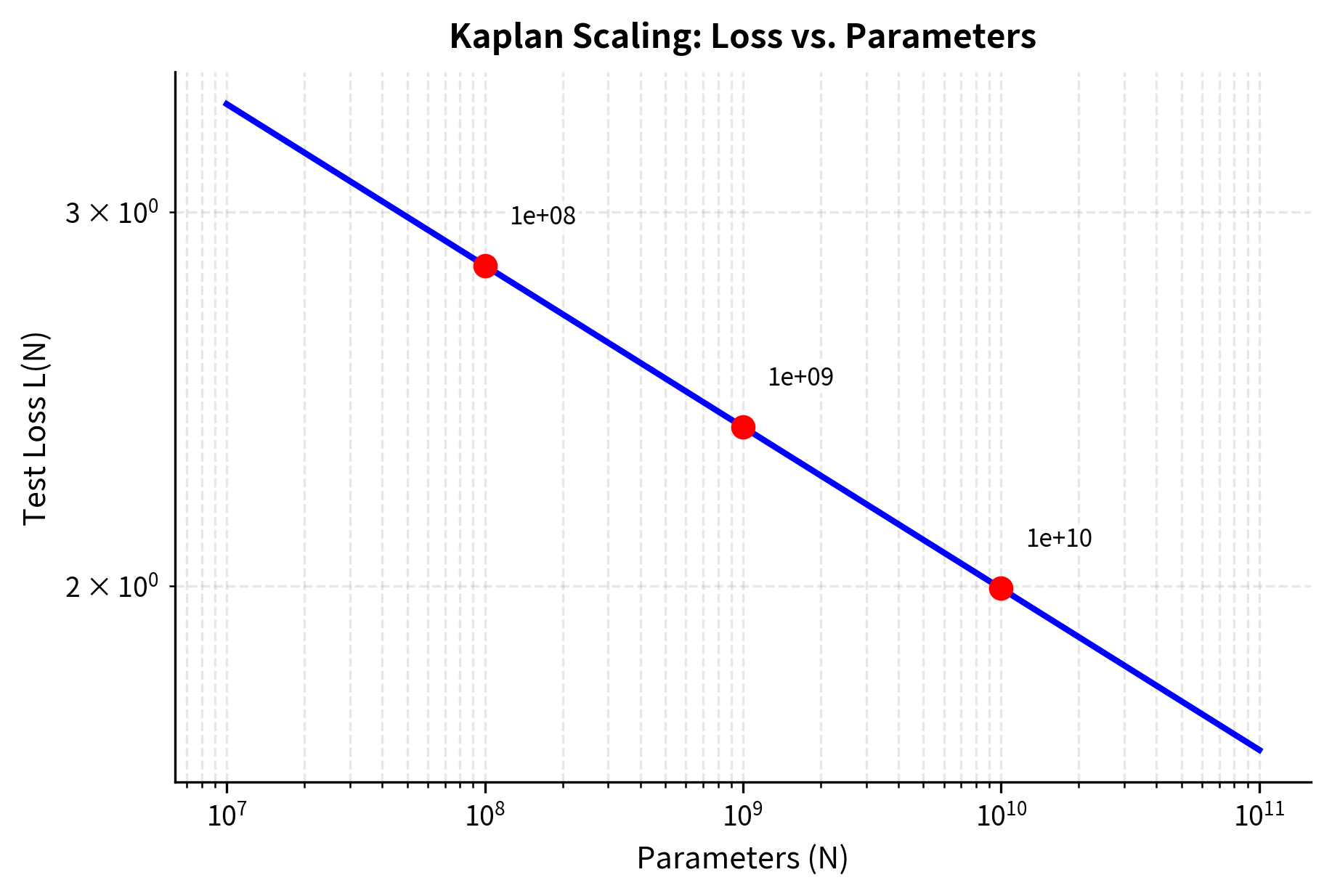
The linearity on log-log axes confirms the power-law relationship. This was not obvious beforehand. The loss could have plateaued, shown diminishing returns, or shown more complex behavior. Instead, the relationship holds remarkably cleanly across four orders of magnitude in model size. The straight line you observe when plotting both axes on logarithmic scales is the defining signature of a power law, and its consistency across such a wide range suggests that the underlying phenomenon reflects something fundamental about how neural networks learn from data.
Loss vs. Data
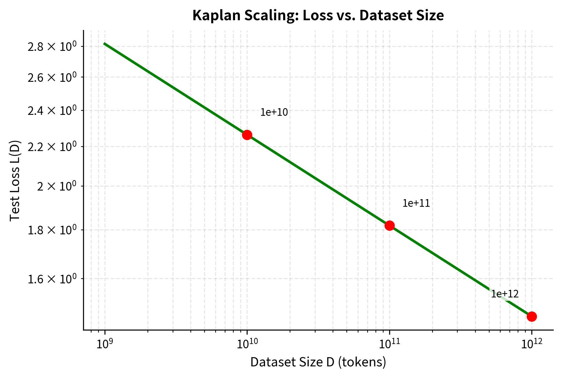
The second scaling law describes how performance improves with more training data. This addresses a complementary question to parameter scaling: if you gather more text to train on, how much better will your model become? Understanding this relationship is crucial because data collection has its own costs. Curating high-quality training corpora requires substantial effort, and some domains have limited data availability.
The intuition behind data scaling is similar to parameter scaling but works differently. When you train on a small dataset, the model sees only a limited sample of language patterns. Common constructions appear often enough to learn well, but rarer phenomena (unusual vocabulary, domain-specific expressions, complex reasoning patterns) may appear too infrequently for reliable learning. As the dataset grows, these rare patterns appear more often, giving the model chances to learn them. Eventually, even very large datasets become saturated. The most common patterns are already learned, and additional data mainly provides more examples of patterns you already captured rather than genuinely new information.
When the model is large enough that it won't overfit (effectively infinite capacity), the loss follows:
where:
- : the cross-entropy loss on held-out text
- : the number of tokens in the training set (the total amount of text the model learns from)
- : a fitted constant representing the characteristic data scale (approximately tokens)
- : the data scaling exponent (approximately 0.095), governing how quickly loss improves with more data
The formula's structure mirrors the parameter scaling law, with serving as the characteristic data scale, similar to how serves as the characteristic parameter scale. This parallel structure isn't coincidental. It reflects the symmetric role that model capacity and data quantity play in determining what a neural network can learn. The characteristic scale tokens represents roughly 54 trillion tokens, an enormous amount of text that far exceeds any practical training corpus. This large value ensures that the ratio remains well above 1 for realistic datasets, producing the predictable decay in loss as data increases.
This follows the same intuition as parameter scaling: each additional training token gives diminishing returns, but the larger exponent () means loss responds more to data increases than parameter increases when measured separately.
The fitted parameters are:
Notice that (0.095 vs 0.076). This comparison shows something important about how sensitive loss is to each resource. With a larger exponent, each multiplicative increase in data produces a bigger drop in loss than the same increase in parameters. Specifically, for the same increase (say, 10x), data scaling reduces loss by a factor of while parameter scaling reduces it by only . Loss improves faster per unit increase in data than in parameters when measured separately. However, as we'll see shortly, this doesn't mean you should prefer more data over larger models when compute is constrained, because the cost of processing more data must be factored into the optimization.
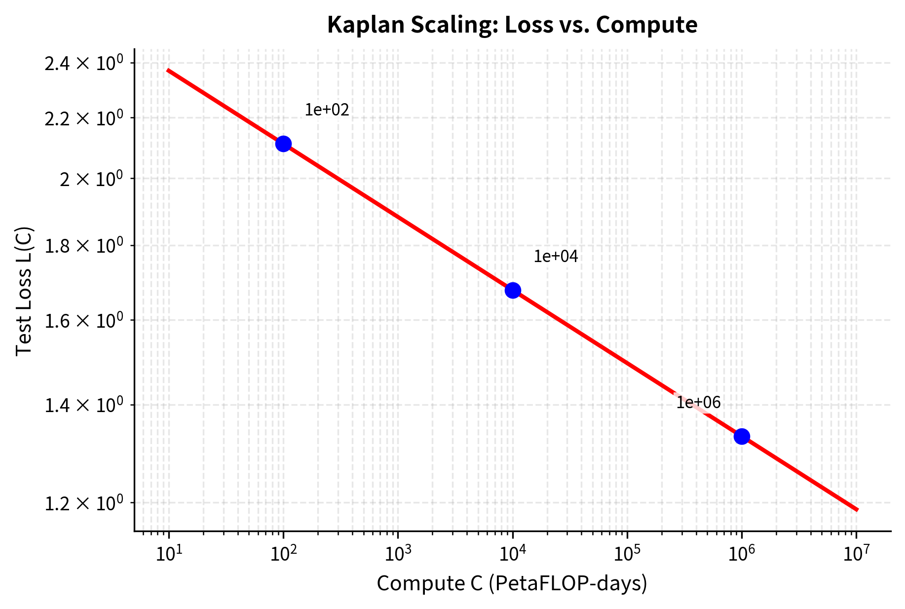
Loss vs. Compute
The third scaling law relates loss directly to the compute budget. This is perhaps the most practically important relationship because compute (measured in GPU-hours, dollars, or energy consumption) is the fundamental constraint that organizations face when training models. Unlike parameters, which can be chosen freely, or data, which can often be collected or synthesized, compute represents a hard resource limit.
Understanding how loss scales with compute means recognizing that compute is a derived resource, not a fundamental one. You don't directly spend compute; instead, you spend it indirectly by choosing a model size (which determines compute per forward-backward pass) and a number of training steps (which determines how many passes you perform). The compute budget constrains the product of these choices, creating a tradeoff. You can train a large model for few steps or a small model for many steps, but you cannot train a large model for many steps within a fixed compute budget.
When training is optimally allocated between model size and training steps, the loss follows:
where:
- : the cross-entropy loss on held-out text
- : the total compute budget measured in PetaFLOP-days (one PetaFLOP-day equals floating-point operations performed continuously for one day)
- : a fitted constant representing the characteristic compute scale (approximately PetaFLOP-days)
- : the compute scaling exponent (approximately 0.050)
The characteristic compute scale PetaFLOP-days represents an enormous amount of computation, roughly 310 million PetaFLOP-days. To put this in perspective, training GPT-3 required approximately 3,640 PetaFLOP-days, which is about five orders of magnitude smaller than . This large characteristic scale ensures that practical training runs operate in the regime where the ratio is much greater than 1, producing meaningful loss values that decrease predictably with more compute.
The compute exponent is smaller than both and because compute is a derived resource. It gets split between making the model larger (more parameters) and training longer (more data passes). The compound effect means each 10x increase in compute yields less loss reduction than a 10x increase in parameters or data alone.
The fitted parameters are:
To understand why the compute scaling works, consider that total compute is approximately . The factor of 6 accounts for roughly two operations per parameter in the forward pass and four in the backward pass (computing gradients for both activations and weights). This relationship comes from the arithmetic of matrix multiplications: each parameter participates in operations during both forward and backward passes, with the backward pass requiring roughly twice the computation of the forward pass to compute gradients. The factor of 6 is an approximation that works reasonably well across typical transformer architectures and training configurations, though the exact multiplier can vary with specific implementation details. This means compute constrains the product of model size and data, forcing a tradeoff between the two.
The compute exponent is smaller than both and . This makes sense: compute is spent on both larger models and more training steps, so its effect is spread across multiple factors. When you increase compute, you gain both from having more parameters (benefiting from the exponent) and from seeing more data (benefiting from the exponent), but neither benefit is realized fully because the compute is divided between them. The key insight is that this relationship only holds when you allocate compute optimally, which brings us to Kaplan's most consequential finding.
The Unified Scaling Law
The individual scaling laws describe performance in idealized settings: infinite data, infinite compute, or optimal allocation. In practice, models train with finite resources across all dimensions. A model might have limited parameters due to hardware constraints, limited data due to collection challenges, and limited compute due to budget restrictions. The unified scaling law addresses this realistic scenario by combining all three factors into a single predictive equation.
The challenge in formulating such a law is figuring out how different constraints interact. If you have a large model but limited data, the model may overfit or fail to use its full capacity. If you have abundant data but a small model, the model may underfit and fail to capture the complexity in the data. The unified law must capture these interactions while reducing to the individual laws in the appropriate limits.
Kaplan et al. proposed a unified equation that combines all three factors:
where:
- : the predicted loss as a function of both model size and data size
- : non-embedding parameters
- : dataset size in tokens
- : the characteristic scales from the individual scaling laws
- : the scaling exponents (0.076 and 0.095 respectively)
- : the ratio of exponents (approximately 0.8), which balances the relative contributions of model and data limitations
- The brackets : the outer exponent applied after summing the two limitation terms, converting the combined constraint into a loss prediction
The formula's structure reveals how parameter and data constraints combine mathematically. Consider the expression inside the brackets: it sums two terms, each representing a different kind of limitation. The term captures the model's capacity limitation, representing how far the current model size is from the characteristic scale, adjusted by the ratio of exponents to ensure consistent units when adding to the data term. The second term, , captures the data limitation in a parallel fashion. Adding them inside the brackets before applying means that whichever constraint is more binding will dominate. You cannot compensate for too little data with a larger model, or vice versa.
This additive structure inside the brackets creates what mathematicians call a "soft minimum" behavior. When one term is much larger than the other, the sum is dominated by that term, and the loss depends primarily on the binding constraint. When both terms are comparable, both constraints matter, and the loss reflects a genuine interaction between model capacity and data availability. This matches our intuition about how training should behave: you need both sufficient model capacity and sufficient data to achieve good performance.
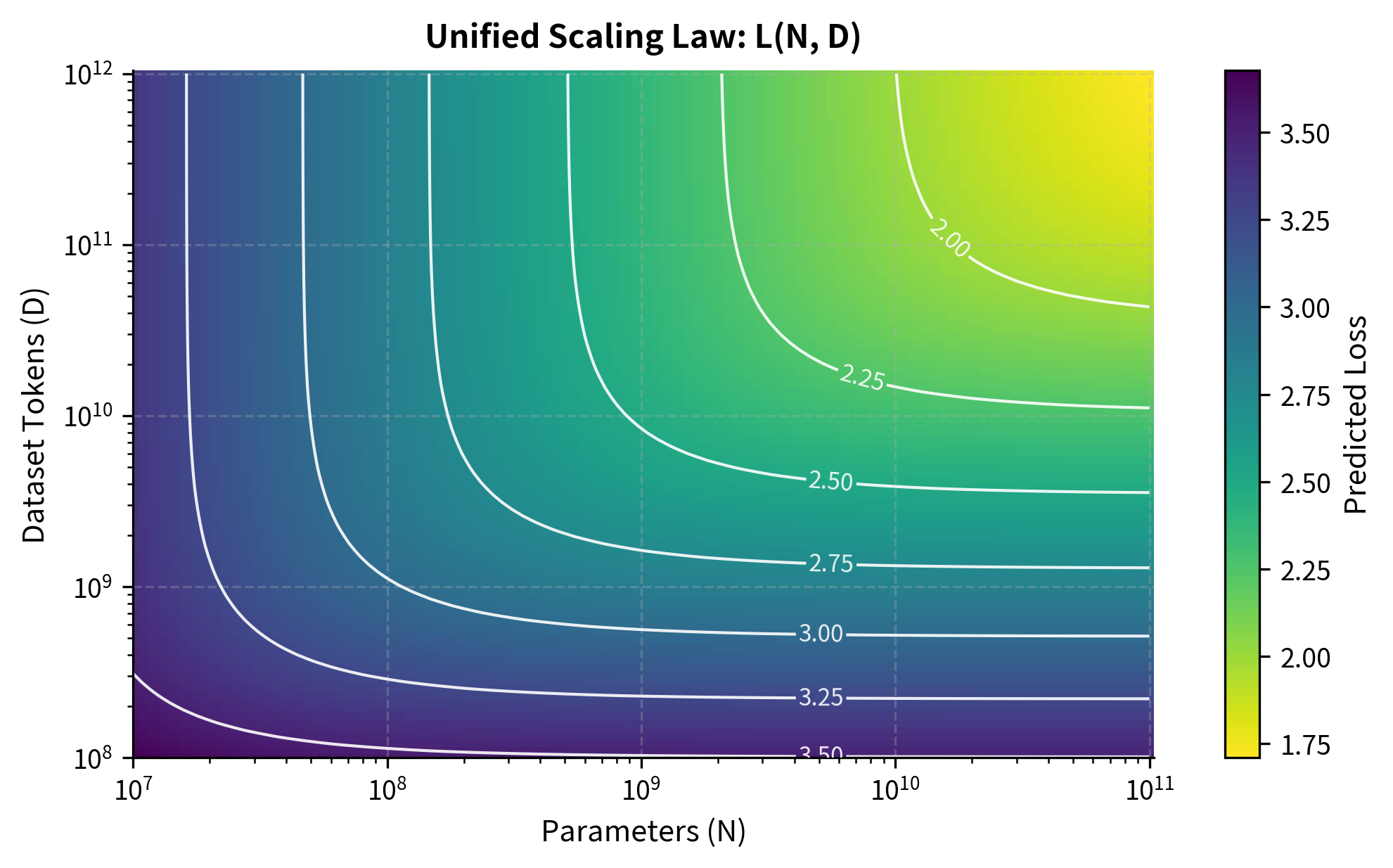
This formula captures an important insight: there's an effective data-to-model ratio that determines performance. A large model on too little data leads to overfitting (the model can't learn effectively from limited signal). Training a small model on too much data leads to a different kind of inefficiency: the model saturates and additional data provides diminishing returns.
The unified law also reveals the irreducible loss component. Even with infinite parameters and infinite data, some entropy remains in natural language that no model can predict. This represents the fundamental unpredictability of language itself.
Optimal Compute Allocation
Kaplan's most influential finding was their guidance on allocating a fixed compute budget between model size and training data. This question is very practical: given a budget of one million dollars worth of GPU time, should you train a modest model for a long time on lots of data, or should you train a very large model for a shorter time on less data? Before scaling laws, practitioners relied on intuition and trial-and-error. Kaplan's analysis provided a principled answer backed by empirical evidence.
The derivation of optimal allocation starts from the fact that compute constrains the product of model size and data: . This means that for a fixed compute budget, increasing necessarily decreases (the number of training tokens seen). The question becomes: what ratio of to minimizes loss for a given ?
Given a compute budget , the optimal model size and dataset size follow:
where:
- : the optimal number of parameters for a given compute budget
- : the optimal number of training tokens for that same budget
- : the total compute budget in PetaFLOP-days
- : denotes proportionality. The left side scales with the right side up to a constant factor
- The exponent 0.73: derived from fitting optimal configurations, indicates parameters should grow faster than the square root of compute
- The exponent 0.27: the complementary exponent for data scaling, since reflects the constraint
These exponents sum to 1.0, which follows from the compute relationship . Taking logarithms: . If we write and , then , requiring . This mathematical constraint ensures consistency: you cannot independently choose how both parameters and data scale with compute, because compute is defined as their product. Notice the stark imbalance: 73% of the compute scaling goes toward larger models, while only 27% goes toward more data.
The asymmetry in these exponents reflects Kaplan's central finding: larger models are more sample-efficient. A bigger model extracts more learning from each training token it sees. This means that as you scale up compute, you should primarily invest in model size rather than training duration. The intuition is that a larger model has more capacity to represent complex patterns, so it can learn those patterns from fewer examples. A smaller model, by contrast, needs to see the same patterns many times before it can reliably capture them.
When your compute budget increases by 10x, you should increase model size by approximately and training tokens by only . Larger models are more sample-efficient. They extract more learning from each token they see.
This recommendation drove concrete decisions. For GPT-3, OpenAI chose a 175B parameter model trained on 300B tokens. Following Kaplan's guidance meant prioritizing a very large model over training on more data.
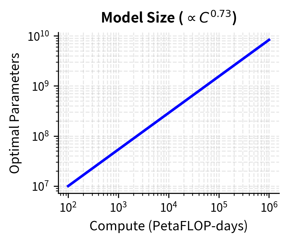
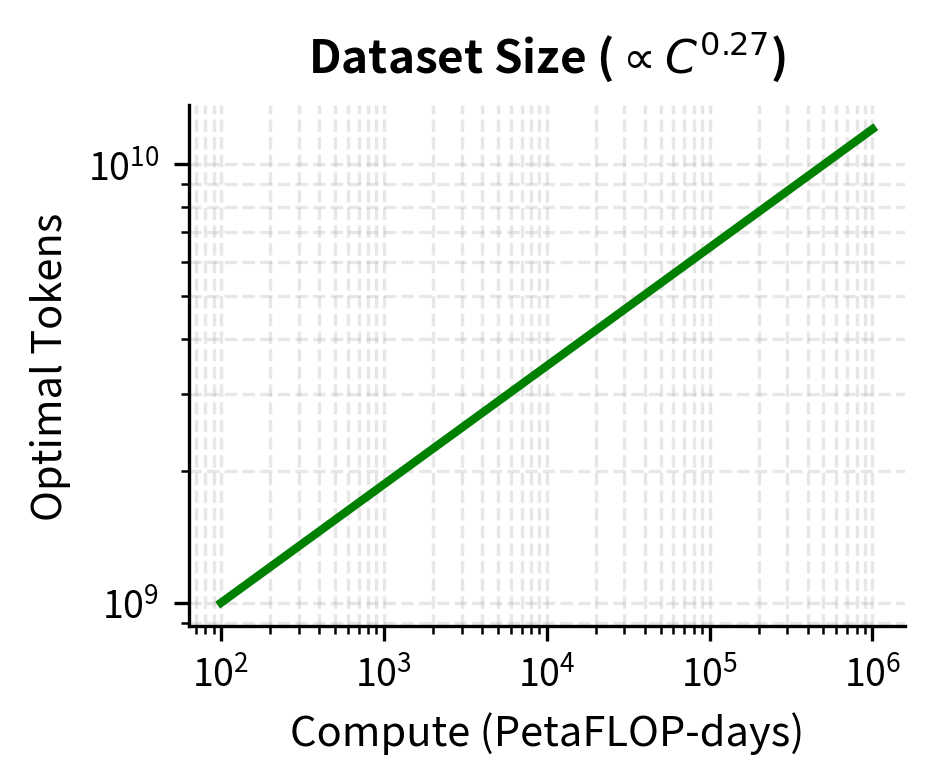
The visual contrast is striking. As compute increases 10,000x (from to PF-days), optimal model size increases by roughly 2500x while optimal dataset size increases by only about 20x. This asymmetry reflects Kaplan's core finding: bigger models learn more efficiently.
Worked Example: Allocating a Compute Budget
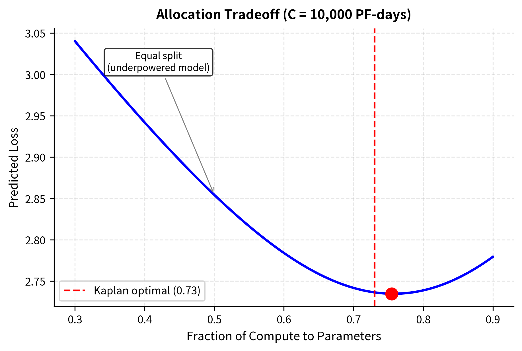
Let's work through a concrete example to see how these scaling laws guide practical decisions. Suppose you have 10,000 PetaFLOP-days of compute available, a substantial budget representing perhaps several million dollars worth of GPU time. How should you allocate it between model size and training data?
First, establish a baseline calibration. The scaling laws provide proportionalities rather than absolute values, so we need reference points to anchor our calculations. From Kaplan's experiments, a reasonable reference is that 100 PetaFLOP-days is roughly appropriate for training a 10 million parameter model on 1 billion tokens. These numbers serve as our calibration baseline. We'll scale up from this known point using the power-law exponents.
First, we need baseline calibration points. From Kaplan's experiments, a reasonable reference is that 100 PetaFLOP-days is roughly appropriate for training a 10 million parameter model on 1 billion tokens. Using the scaling exponents:
where:
- : the optimal parameter count for compute budget
- : the optimal token count for compute budget
- : reference values at a known compute level (here, 10M parameters and 1B tokens)
- : the reference compute level (here, 100 PetaFLOP-days)
- The ratio : represents how many times larger your budget is compared to the reference
- The exponents 0.73 and 0.27: the Kaplan optimal allocation exponents, determining how aggressively each resource scales with compute
The calculation proceeds by first computing the ratio of our budget to the baseline budget: . This tells us we have 100 times more compute than the baseline case. We then raise this ratio to each power-law exponent to determine how much each resource should scale. For parameters, , meaning we should use approximately 29 times more parameters than the baseline. For data, , meaning we should use approximately 3.5 times more data than the baseline.
With 10,000 PetaFLOP-days, Kaplan's scaling laws recommend training roughly a 1.4 billion parameter model on about 4.3 billion tokens. The tokens-per-parameter ratio is particularly telling: at only about 3 tokens per parameter, the model sees each parameter's worth of data only a few times. This low ratio reflects the "train big, don't overtrain" philosophy that emerged from this work. Traditional machine learning wisdom suggested that models need many samples per parameter to avoid overfitting, but Kaplan's analysis showed that for language models, the opposite approach works better. Make the model large and stop training relatively early.
Notice the tokens-per-parameter ratio is only about 3. The model sees each parameter's worth of data only a few times. This low ratio reflects the "train big, don't overtrain" philosophy that emerged from this work.
Comparing Scaling Behavior
To appreciate how the three scaling laws interact and to develop intuition for their relative magnitudes, it helps to visualize them together on a common scale. This comparison shows the hierarchy of exponents and explains why optimal compute allocation favors model size over data.
When we plot all three scaling relationships on the same axes, we normalize each curve to pass through the point (1, 1), representing a baseline case. This allows us to compare slopes: a steeper slope means faster loss improvement per unit increase in the resource. The steepness of each curve directly reflects its corresponding exponent. Larger exponents produce steeper downward slopes on log-log axes.
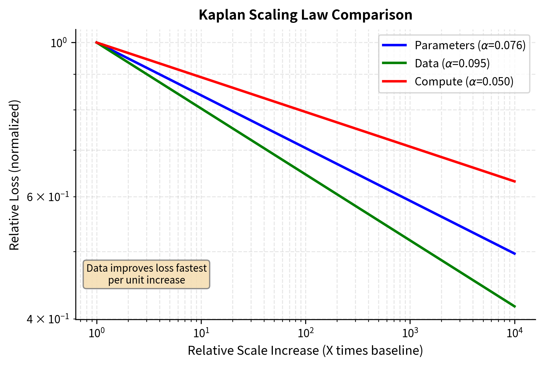
At first glance, you might think this figure contradicts the recommendation to scale models over data. After all, the data curve drops fastest. Remember that the constraint is compute, not the resource itself. This is a subtle but important distinction. The x-axis shows multiplicative increases in each resource independently, but in practice, you cannot independently scale data without consuming compute. Increasing parameters by 10x costs proportionally more compute than increasing data by 10x (roughly). When you factor in these costs, the optimal allocation still favors larger models.
The answer is that data scaling requires compute (you must process each token), while parameter scaling has a fixed cost per training step regardless of model size. Roughly speaking, the compute per step scales with , but the total compute means the relationship is multiplicative. The optimal allocation calculation properly accounts for these costs and determines that investing in model size yields better returns per unit of compute than investing in more training data.
Predicting Performance at Scale
One of the most useful applications of scaling laws is extrapolation. If the power laws hold, you can predict performance at scales you haven't yet trained. This turns scaling laws from retrospective descriptions into planning tools. Rather than running many expensive experiments to find the best configuration, you can train a few small models, fit the scaling parameters, and extrapolate to predict how larger models will perform.
Kaplan et al. used this approach to estimate the performance of models orders of magnitude larger than any that existed at the time. This extrapolation informed the decision to build GPT-3 and provided confidence that the investment would yield proportional returns.
These predictions show how loss decreases as models scale from 1 billion to 1 trillion parameters. The improvement percentages represent how much lower the loss is compared to a 100 million parameter baseline. Each 10x increase in parameters yields approximately a 16% relative improvement, consistent with the exponent.
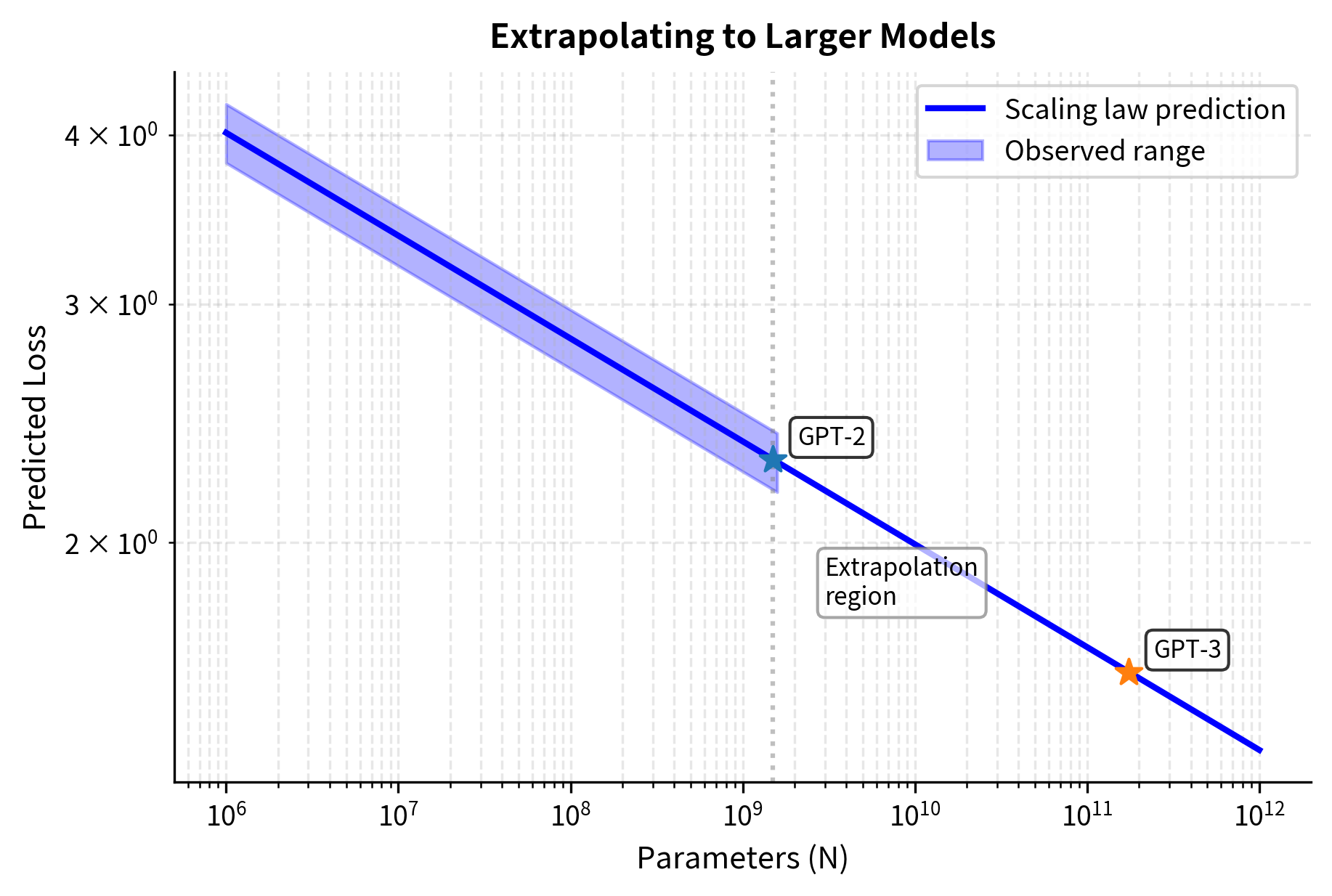
At 1 trillion parameters, the model achieves roughly 16% lower loss than the 100M baseline, a meaningful improvement that reflects the diminishing returns inherent in power-law scaling. While 16% might sound modest, remember that cross-entropy loss relates logarithmically to perplexity. A 16% reduction in loss translates to a substantial reduction in perplexity, which correlates with noticeably better text generation quality. This finding influenced strategic decisions about how far to push scale.
How reliable these extrapolations are depends on whether the power-law relationships continue to hold at larger scales. If there are phase transitions, saturation effects, or architectural limitations that emerge at scale, the predictions could be systematically wrong. This uncertainty motivated ongoing research into whether scaling laws exhibit any departures from pure power-law behavior.
Implementation: Scaling Law Calculator
Let's build a practical tool for working with Kaplan scaling laws. This implementation encapsulates all the key relationships we've discussed into a reusable class that can predict losses and compute optimal allocations:
The predicted losses demonstrate how the scaling law captures performance differences across model sizes. GPT-2 Small's higher loss compared to GPT-2 XL reflects the consistent power-law improvement. The much larger GPT-3 shows further gains that align with the α_N = 0.076 exponent. These predictions allow researchers to estimate whether building a larger model is worth the investment before committing the resources.
Now let's use the optimal allocation function to explore different compute budgets:
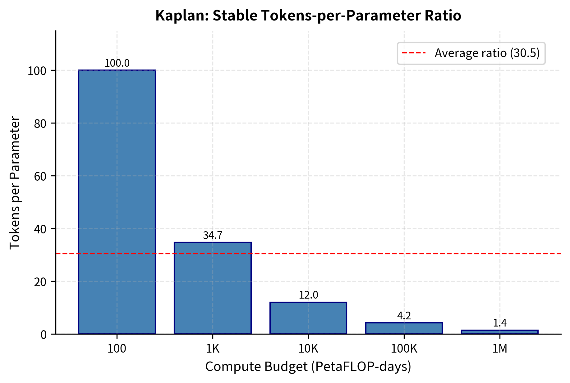
This table shows how Kaplan's optimal allocation shifts the balance toward larger models as compute increases. At 1 million PetaFLOP-days, the recommended model has over 100 billion parameters but trains on only about 20 billion tokens, a ratio that seemed counterintuitive before scaling laws were established. The conventional wisdom had been that models needed many examples per parameter to avoid overfitting, but Kaplan's analysis showed that for language models, the optimal strategy is the opposite: build very large models and train them for relatively few steps.
The tokens-per-parameter ratio remains stable across scales, hovering around 3-4 tokens per parameter. This is far below what many practitioners assumed was necessary before scaling laws were established.
Limitations and Impact
The Kaplan scaling laws helped us understand neural language models, but they had significant limitations that later research would address.
The main limitation was their experimental methodology for measuring optimal allocation. Kaplan et al. estimated optimal model and data sizes by training models for different numbers of steps and seeing which configurations gave the best loss for a given compute budget. However, they did not train any models fully to convergence. They relied on early training dynamics to extrapolate optimal configurations. This choice led to systematic bias toward larger models and shorter training runs. The Chinchilla scaling laws, which we'll explore in the next chapter, would later demonstrate that training models much longer on more data is actually more compute-efficient than Kaplan's analysis suggested.
Another limitation was the narrow scope of experiments. All experiments used a single architecture family (decoder-only transformers), a single dataset (WebText2), and a single domain (English web text). The fitted constants and even the exponents may not generalize to encoder models, different languages, or specialized domains like code or scientific text. Subsequent work has shown that optimal scaling behavior does vary across these dimensions.
The treatment of compute was also simplified. Kaplan measured compute in PetaFLOP-days, aggregating all operations equally. In practice, different operations have different hardware efficiency, and memory bandwidth often matters more than raw FLOPS for large models. The relationship that Kaplan used as an approximation is reasonable but not exact across all architectures and batch sizes.
Despite these limitations, Kaplan's work had a major impact. For the first time, researchers had quantitative guidance for resource allocation decisions. The framework of power-law scaling became standard vocabulary in the field, and the methodology of fitting scaling laws to predict large-model performance became essential for compute-limited research planning. GPT-3's architecture and training decisions were directly informed by these scaling laws, demonstrating their practical influence on billion-dollar training runs.
The work also raised questions that motivate ongoing research: Why do power laws emerge at all? Are there phase transitions or inflection points hidden at larger scales? What determines the exponents, and can we design architectures with better scaling? These questions relate to the emergence phenomena we'll explore in later chapters.
Summary
The Kaplan scaling laws showed that language model performance follows predictable power-law relationships across three dimensions:
- Loss vs. parameters: , meaning doubling model size reduces loss by about 5%
- Loss vs. data: , with slightly steeper improvement per unit of data
- Loss vs. compute: , assuming optimal allocation
To interpret these exponents: a 10x increase in any factor reduces loss by , so parameters give improvement, data gives , and compute gives improvement.
The key practical finding was the optimal allocation formula: when scaling up compute, increase model size as and data as . This prescription (scale models faster than data) shaped the development of GPT-3 and showed that larger models are more sample-efficient.
These relationships held cleanly across four orders of magnitude in the original experiments, allowing extrapolation to scales that hadn't yet been trained. However, the methodology for determining optimal allocation had systematic limitations that later work would revise. The next chapter examines the Chinchilla scaling laws, which challenged Kaplan's recommendations and showed that models like GPT-3 were actually undertrained relative to their size.
Key Parameters
The key parameters for Kaplan scaling laws are:
- α_N (0.076): Parameter scaling exponent. Determines how quickly loss decreases as model size increases.
- α_D (0.095): Data scaling exponent. Governs the rate of loss improvement with more training tokens.
- α_C (0.050): Compute scaling exponent. Controls loss reduction when compute budget increases with optimal allocation.
- N_c, D_c, C_c: Characteristic scale constants. Fitted values representing the scale at which each resource reaches a reference loss level.
- Allocation exponents (0.73, 0.27): Optimal compute allocation. Specify how to split compute budget between larger models and more data.
Quiz
Ready to test your understanding? Take this quick quiz to reinforce what you've learned about Kaplan scaling laws.

Comments