Power Laws in Deep Learning: Understanding Neural Scaling

Throughout this book, we've built increasingly sophisticated language models, from simple n-gram models through BERT and GPT architectures to modern designs like LLaMA and Mistral. A natural question emerges: how does model performance change as we scale up? More parameters, more data, more compute. What returns do these investments yield?

The answer lies in a deceptively simple mathematical relationship that governs neural network scaling: the power law. Understanding power laws transforms how we think about training language models. Instead of guessing at the right model size or dataset, we can predict performance across orders of magnitude, make informed resource allocation decisions, and understand the fundamental constraints that govern what's possible with current approaches.

This chapter establishes the mathematical foundations of power laws, explores why they appear so universally in deep learning, and develops the intuition you'll need to interpret the scaling laws we'll examine in subsequent chapters.

Before we can understand how neural networks scale, we need to establish the mathematical vocabulary that describes scaling relationships. The concept we're after is the power law—a particular type of functional relationship that, as you'll soon see, captures something essential about how complex systems behave as they grow.

A power law describes a relationship where one quantity varies as a power of another. This might sound abstract at first, so let's ground it with an intuition. Imagine you're measuring how some output changes as you adjust an input. In the simplest case of a linear relationship, doubling the input doubles the output. The world of power laws is different and more interesting. If you double the input, the output doesn't simply double. Instead, it changes by a fixed multiplicative factor that depends on a special number called the exponent. This exponent is the heart of a power law: it tells you exactly how sensitive the output is to changes in the input.

The general form is:

Let's unpack each component of this equation to build a complete understanding:

• $y$: the dependent variable (output quantity). This is what we're measuring or predicting. In deep learning contexts, it's often the loss of our model.
• $x$: the independent variable (input quantity). This is what we control or vary: parameters, data, compute, or training steps.
• $a$: the coefficient, which sets the overall scale of the relationship. Think of this as calibrating where the curve sits vertically. If $a$ is large, the entire curve shifts upward; if $a$ is small, it shifts downward. The coefficient captures baseline performance characteristics specific to your architecture, task, or data.
• $b$: the exponent (or scaling exponent), which determines how steeply $y$ changes as $x$ increases. This is the most important parameter for understanding scaling behavior. The exponent tells us whether improvements come quickly or slowly as we add resources.

When $b$ is negative, we often write this as:

where $\alpha = -b > 0$ represents the positive scaling exponent. This alternative notation proves convenient in deep learning contexts because it makes the relationship more immediately interpretable. When written this way, we can see at a glance that as $x$ increases, $y$ decreases, which matches our intuition that adding more parameters or data should improve, that is, lower, our loss. The positive exponent $\alpha$ directly tells us the rate of this improvement.

Now that we have the basic form, let's understand what makes power laws genuinely special compared to other mathematical relationships you might encounter. Consider three common functional forms and how they behave:

Linear: $y = ax + c$. Doubling $x$ adds a fixed amount to $y$. If you go from 100 to 200 parameters, you get the same absolute improvement as going from 1 billion to 1 billion plus 100 parameters. This kind of relationship treats all additions equally, regardless of scale. However, this doesn't match how neural networks actually behave.

Exponential: $y = a \cdot e^{bx}$. Doubling $x$ multiplies $y$ by a fixed factor that grows explosively. Small changes in $x$ can produce enormous changes in $y$. Exponential relationships describe radioactive decay, compound interest, and viral spread, situations where growth feeds on itself. Neural network scaling doesn't show this kind of explosive behavior.

Power law: $y = ax^b$. Multiplying $x$ by any factor $k$ multiplies $y$ by $k^b$. The key insight is that power laws respond to proportional changes, not absolute changes. Whether you're scaling from 10 million to 100 million parameters or from 10 billion to 100 billion parameters, the proportional change is the same, a factor of 10, and therefore the proportional effect on the output is the same.

The distinctive feature of power laws is scale invariance: the relationship between proportional changes stays constant regardless of where you are on the curve. A 10× increase in model parameters produces the same proportional decrease in loss whether you're going from 100M to 1B parameters or from 1B to 10B parameters. This property matters because it means power laws look the same at every scale. Zoom in or zoom out on a power law relationship, and the shape remains unchanged. This scale invariance is what enables us to make predictions about enormous models based on experiments with much smaller ones.

Understanding the mathematical form of power laws is only the beginning. The practical key to identifying, validating, and working with power laws is a transformation that converts these curved relationships into straight lines. This transformation bridges theory and practice.

Taking the logarithm of both sides of $y = ax^b$ reveals the hidden linear structure:

Let's trace through this derivation step by step to see where each piece comes from. We start with the power law $y = ax^b$ and take the logarithm of both sides. The left side simply becomes $\log y$. For the right side, we apply two fundamental properties of logarithms. First, the product rule tells us that $\log(ab) = \log a + \log b$, meaning the logarithm of a product is the sum of the logarithms. Second, the power rule tells us that $\log(x^b) = b \log x$. When we take the log of something raised to a power, the exponent comes down as a multiplier.

Applying these rules transforms our power law into a linear equation. To see the linear structure more clearly, let's introduce new variables. Let $Y = \log y$ and $X = \log x$. Our equation becomes:

This is unmistakably the equation of a straight line in slope-intercept form. Each component has a clear geometric interpretation:

• $\log y$: the logarithm of the dependent variable, which becomes our new y-axis in the transformed space
• $\log a$: a constant term that becomes the y-intercept when we treat this as a linear equation—where the line crosses the vertical axis
• $b$: the power law exponent, which becomes the slope of our line—how many units $\log y$ changes for each unit change in $\log x$
• $\log x$: the logarithm of the independent variable, which becomes our new x-axis in the transformed space

This transformation works because of the logarithm's key properties: $\log(ab) = \log a + \log b$ and $\log(x^b) = b \log x$. The result is a linear equation in $\log x$ and $\log y$. If you plot data on log-log axes, where both axes are logarithmic, and the relationship is a power law, you'll see a straight line with slope $b$ and y-intercept $\log a$.

Why does this matter so much? Because straight lines are easy to work with. We have well-established tools for analyzing, fitting, and extrapolating linear relationships. By transforming power laws into lines, we gain access to this entire toolkit.

This transformation has practical implications:

• Detection: If your data forms a straight line on log-log axes, you've found a power law. This gives you a simple visual test: plot your scaling data with logarithmic scales on both axes, and look for linearity.
• Parameter estimation: The slope gives you the exponent directly. No complex optimization needed—basic linear regression suffices.
• Extrapolation: Linear extrapolation in log space corresponds to power law extrapolation in linear space. We can extend a straight line with confidence. The log-log transformation lets us translate that confidence to power law predictions.

Let's see this concretely with a worked example that shows how to reason about power law scaling. Suppose loss $L$ decreases with compute $C$ according to:

Before diving into the math, let's understand what this equation is telling us. The coefficient 5.4 represents the loss we would observe at $C = 1$ (one FLOP of compute), which is of course unrealistically small. No real model trains with one floating-point operation. This coefficient anchors the curve but isn't particularly meaningful on its own. The exponent $-0.05$ is where the action is: it tells us that loss decreases slowly as compute increases, with the negative sign indicating an inverse relationship, meaning more compute leads to less loss, and the small magnitude indicating gradual improvement.

Let's make each term explicit:

• $L$: the model's loss (lower is better)
• $C$: compute budget in FLOPs (floating-point operations)
• $5.4$: the coefficient, representing the loss at $C = 1$
• $-0.05$: the scaling exponent, indicating loss decreases slowly with compute

Taking logs (base 10 for interpretability, since we're used to thinking in powers of 10):

Now we can read off the linear relationship. In log space, our line has y-intercept 0.73 and slope $-0.05$. The slope tells us exactly how log-loss changes as we increase log-compute.

If we increase compute by a factor of 10 (one order of magnitude), this means $\log_{10} C$ increases by exactly 1. The change in log-loss is therefore:

What does a change of $-0.05$ in $\log_{10} L$ mean for actual loss? We can work backwards: if $\log_{10} L$ decreases by $0.05$, then $L$ is multiplied by $10^{-0.05} \approx 0.89$. The new loss is approximately 89% of its previous value, representing an 11% reduction. Each order of magnitude of compute reduces loss by about 11%.

This fixed proportional improvement per order of magnitude is the signature of power law scaling. It doesn't matter whether you're going from $10^{15}$ to $10^{16}$ FLOPs or from $10^{23}$ to $10^{24}$ FLOPs: each tenfold increase in compute buys you the same 11% reduction in loss. This predictability is what makes power laws so valuable for planning.

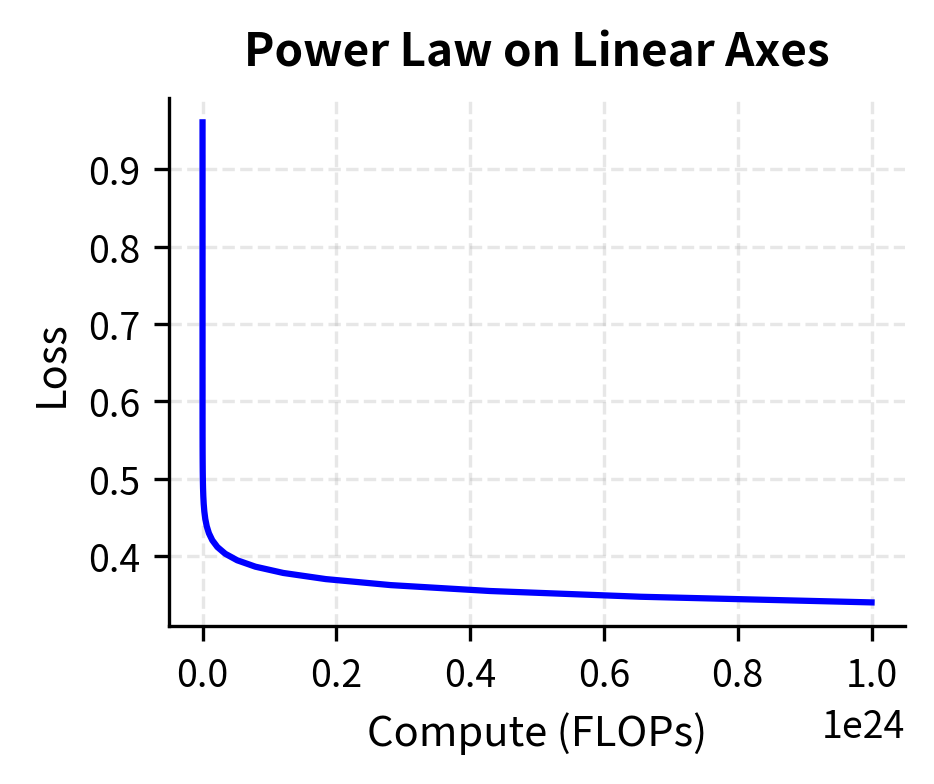
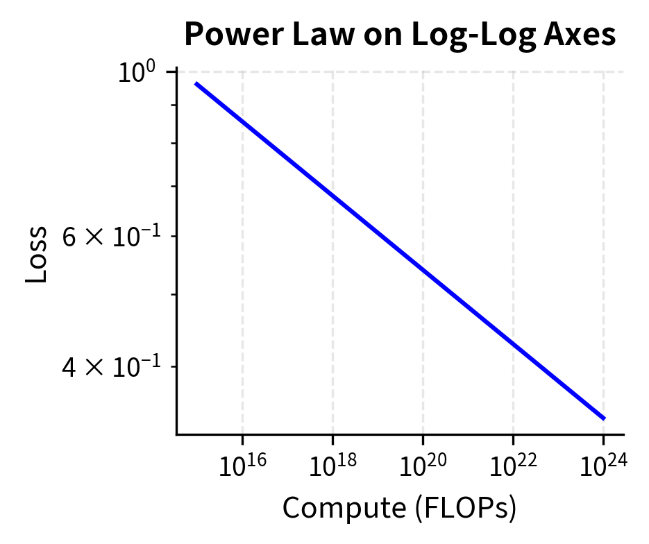
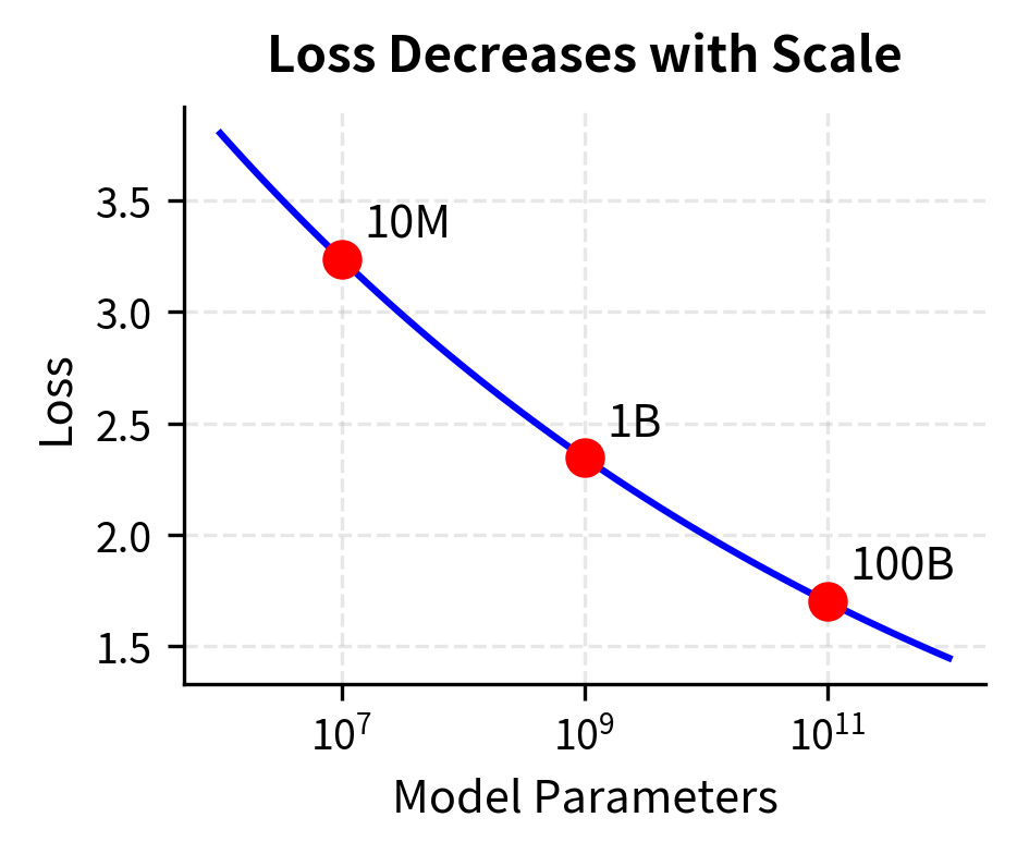
We can visualize this relationship by generating power law data and plotting it on both linear and log-log axes:

The left plot shows the curved relationship typical of power laws on linear axes, while the right plot reveals the elegant simplicity of the log-log representation. The slope of the line in log-log space gives us the exponent $-0.05$ directly. Notice how the curve that appeared complex on linear axes becomes a perfectly straight line once we transform both axes to logarithmic scales. This visual simplicity reflects the mathematical simplicity we derived above: power laws are linear relationships in disguise, and the log-log transformation reveals that hidden linearity.

Power laws aren't new to language modeling. In fact, you've encountered one of the most famous power laws in language already: Zipf's law. This connection is more than historical curiosity—it reveals that power law behavior is woven into the very fabric of language itself.

When we discussed word frequency distributions in earlier chapters, we noted that the frequency of words follows a remarkably consistent pattern. If you rank words by frequency, the $r$-th most common word appears with frequency proportional to $1/r$:

Let's break down what each term means in this linguistic context:

• $f(r)$: the frequency of the word at rank $r$, meaning how many times it appears in a corpus
• $r$: the rank of the word (1 = most common, 2 = second most common, etc.)
• $\alpha$: Zipf's exponent, approximately 1 for most natural language corpora
• $\propto$: "proportional to" (the relationship holds up to a constant factor)

The word "the" appears vastly more often than "cat," which appears vastly more often than "syzygy." This isn't gradual. The most common words dominate text, while the long tail of rare words contributes relatively little to token counts.

The exponent $\alpha \approx 1$ has a striking implication that we can trace through arithmetically. If the most common word appears 1 million times, the 10th most common word appears roughly 100,000 times, which is one-tenth as often, and the 100th most common word appears roughly 10,000 times, which is one-hundredth as often. Each factor of 10 in rank produces a factor of 10 decrease in frequency. This is scale invariance in action: the same proportional pattern repeating across the entire frequency spectrum.

Zipf's law connects directly to the vocabulary problem we explored in Part V. The heavy tail of rare words means that no matter how large your vocabulary, you'll encounter unseen words. This motivated subword tokenization approaches like BPE and WordPiece, which handle rare words by decomposing them into more frequent subunits. In this way, understanding the power law structure of language directly informed the design of modern tokenization systems.

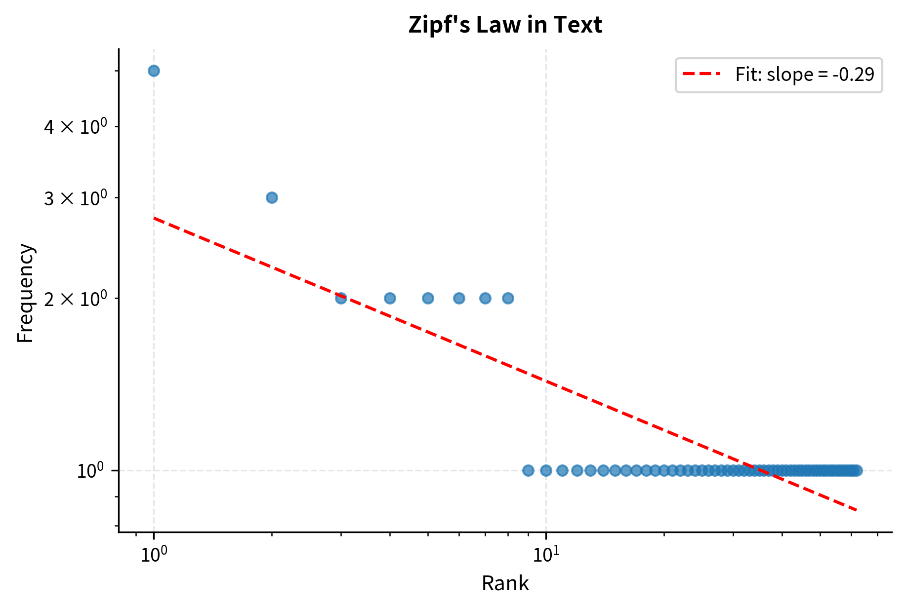
The output shows "language" as the most frequent word in our sample text, appearing 6 times. The fitted Zipf exponent close to 1 confirms Zipf's law holds even for this small corpus. This same mathematical pattern, a power law relationship, governs how neural network performance scales with resources.

To use power laws predictively, we need to estimate the parameters $a$ and $b$ from data. This is where the log-log transformation proves most useful. Instead of wrestling with nonlinear curve fitting, we can use the simple, well-understood tools of linear regression on log-transformed data.

Given data points $(x_i, y_i)$, we transform to $(\log x_i, \log y_i)$ and fit the linear model:

Each component of this equation has a specific role in the fitting process:

• $\log y$: the log-transformed dependent variable—we compute this from our measured loss values
• $\log x$: the log-transformed independent variable—we compute this from our resource measurements (parameters, data, compute)
• $\log a$: the y-intercept in log space, which we'll recover from the regression
• $b$: the slope, which equals the power law exponent directly—this is the number we most care about

Comparing this to the standard linear form $Y = mX + c$ makes the connection explicit. The slope $m$ in our transformed regression equals $b$ (the power law exponent). We read it directly from the regression output. The intercept $c$ equals $\log a$, which we convert back to the original coefficient via exponentiation, giving $a = e^c$, or $a = 10^c$ if using base-10 logarithms.

The regression gives us $b$ (the slope) and $\log a$ (the intercept). From these two numbers, we can reconstruct the entire power law relationship and make predictions for any scale.

However, fitting power laws correctly requires care. Several subtle issues can trip up the unwary analyst:

Use log-transformed data for regression. This point deserves emphasis because it's counterintuitive. You might think, "I want to fit $y = ax^b$, so I should use nonlinear regression to minimize the sum of squared errors in $y$." This approach overweights large values. If your losses range from 10 at small scales to 0.1 at large scales, squared errors at the small end, potentially hundreds, will dwarf squared errors at the large end, which are fractions. The optimizer will focus on matching the high-loss region while ignoring the low-loss region. Fitting in log space minimizes relative errors. It treats a 10% miss at loss 10 the same as a 10% miss at loss 0.1. This is usually what we want when values span many orders of magnitude.

Consider weighted regression. If measurement uncertainty varies across your data range, weighted regression can improve estimates. For instance, if small-scale experiments have lower variance than large-scale ones, you might upweight them accordingly.

Validate with residual analysis. After fitting, examine residuals in log space. If the residuals show systematic patterns, such as being consistently positive at small scales and negative at large scales, this indicates the power law model may not be appropriate. True power law data should produce residuals that scatter randomly around zero.

Let's implement power law fitting and see these principles in action:

Let's test our fitting function on synthetic data where we know the true parameters:

The fitted parameters closely match the true values, with the coefficient recovered as 10.031 (true: 10.0) and exponent as -0.0760 (true: -0.076). The R-squared value of 0.9989 indicates an excellent fit, demonstrating that our log-space regression approach effectively recovers power law parameters even with noisy data.

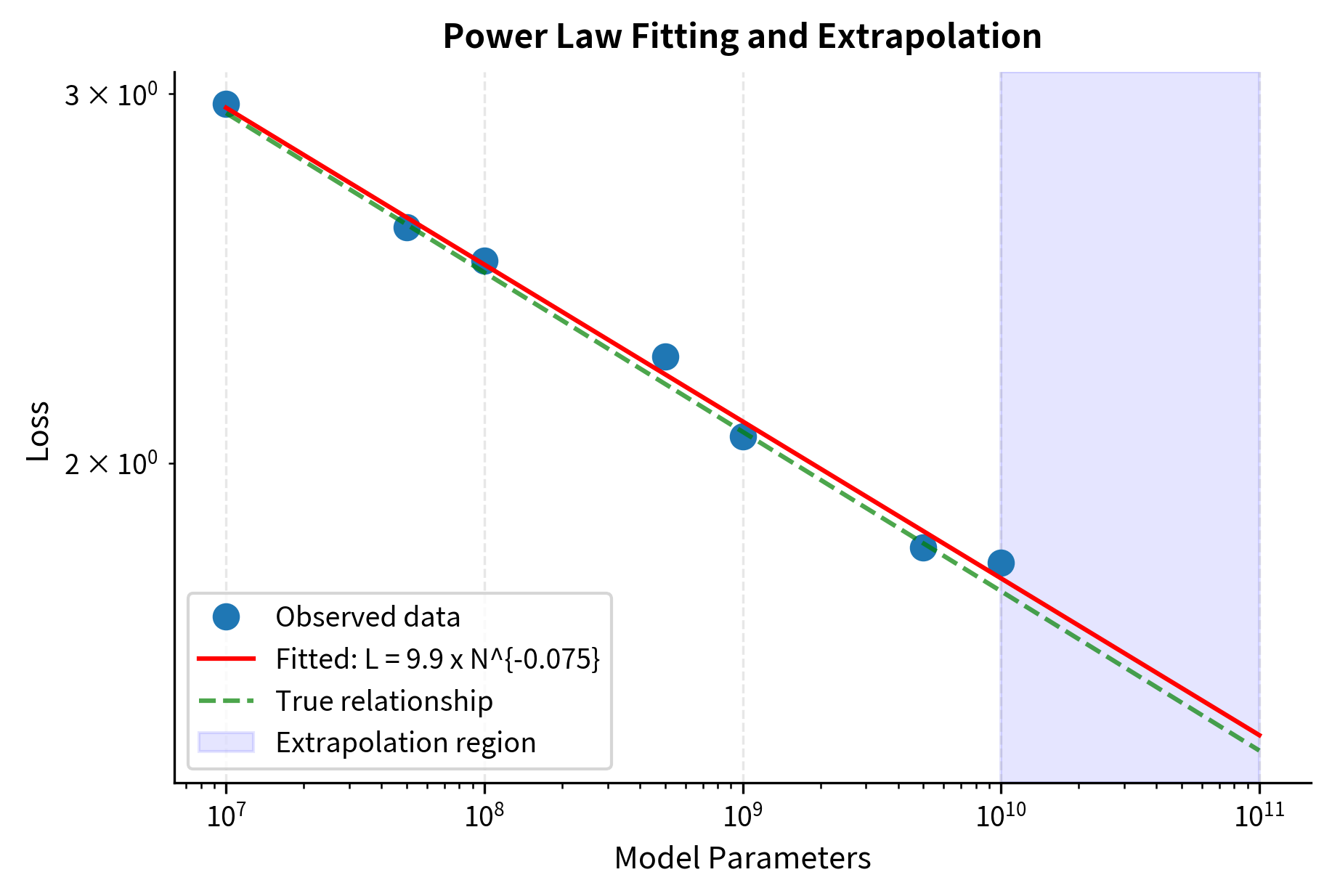
The fit recovers the true parameters with reasonable accuracy. More importantly, it enables extrapolation: we can predict performance for model sizes we haven't trained yet. This predictive power is what makes scaling laws so valuable for planning large language model training.

To validate that our power law fit is appropriate, we should examine the residuals—the differences between observed and predicted values in log space. A good fit produces residuals that scatter randomly around zero with no systematic pattern:

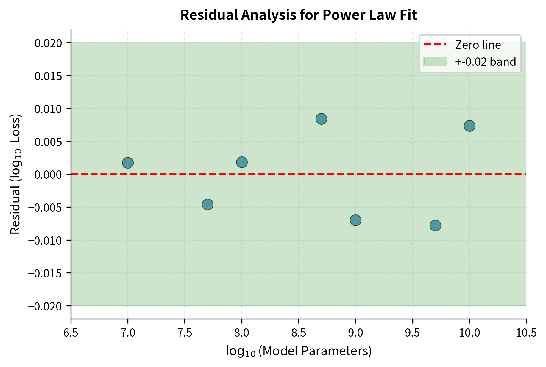
The residuals scatter randomly within a narrow band around zero, confirming that our power law model is appropriate for this data. If we saw a curved pattern in the residuals (e.g., positive at both extremes and negative in the middle), it would suggest the true relationship isn't a simple power law.

One of the most striking aspects of deep learning scaling is how consistently power laws appear. Empirical studies across different model architectures, different datasets, and different tasks repeatedly find power law relationships. This consistency is remarkable and requires explanation. Loss scales as a power law with:

• Number of parameters
• Amount of training data
• Total compute budget
• Training steps (in certain regimes)

This universality requires explanation. Why should such diverse systems exhibit the same mathematical pattern? After all, a transformer trained on code, a recurrent network trained on books, and a mixture-of-experts model trained on web text are very different systems. Yet they all show power law scaling.

Several theoretical perspectives offer insight, each illuminating a different facet of this phenomenon:

Statistical mechanics analogy. Complex systems with many interacting components often exhibit power law behavior as they approach critical points. These critical points are phase transitions where system behavior changes qualitatively. Neural networks, with billions of parameters interacting through nonlinear dynamics, share structural similarities with these systems. Just as water at the critical point exhibits scale-invariant fluctuations, neural networks in training may inhabit a regime where scale-invariant learning dynamics emerge naturally.

Random matrix theory. The Hessian, which is the matrix of second derivatives, of neural network loss functions shows spectral properties connected to random matrix theory. Power law distributions in eigenvalue spectra can translate to power law scaling in learning dynamics. This connection suggests that the high-dimensional geometry of loss landscapes may be responsible for power law behavior.

Feature learning dynamics. As networks train, they progressively learn features of increasing complexity. Simple patterns like edges and common words are learned first; complex patterns like object categories and semantic relationships come later. The marginal difficulty of learning additional features may increase in a way that produces power law returns on additional capacity. Each new feature is harder to learn than the previous one, but not impossibly so. This gradual increase in difficulty manifests as power law scaling.

Bias-variance tradeoff. The decomposition of error into irreducible noise, approximation error, and estimation error can produce aggregate power law behavior over wide ranges. Each component may scale differently, and aggregate power law behavior over wide ranges. The total error we observe is a sum of these components, and under certain conditions, that sum exhibits power law scaling even if the individual components don't.

While no single theory fully explains power law universality, the empirical consistency is robust enough to be practically useful. We'll see in subsequent chapters how specific scaling laws quantify these relationships precisely.

Understanding power laws conceptually helps you reason about scaling decisions. Mathematical formulas are essential, but developing intuition about what those formulas mean allows you to think fluidly about scaling without constantly returning to the equations. Here are key intuitions to develop:

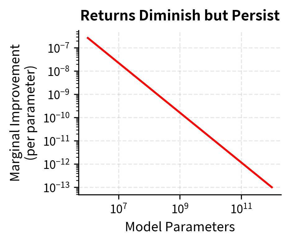
Diminishing returns are inevitable but gradual. A power law of the form $L = aN^{-\alpha}$ with $\alpha > 0$ means each additional parameter contributes less than the previous one. Let's be explicit about each term:

• $L$: the loss we're trying to minimize
• $N$: the number of model parameters
• $a$: a constant that sets the overall scale
• $\alpha$: the positive scaling exponent (with $\alpha > 0$ ensuring diminishing returns)

The negative exponent ensures that as $N$ increases, $L$ decreases, but the rate of decrease slows as $N$ grows larger. The millionth parameter is worth less than the first, but it's not worthless. This gradual decline contrasts sharply with exponential decay, where returns plummet rapidly after an initial period. Power law diminishing returns are persistent. There is always some benefit to scaling further, even if the marginal gain shrinks.

Orders of magnitude matter more than absolute quantities. Power law thinking is multiplicative rather than additive. Going from 1B to 2B parameters gives the same proportional improvement as going from 10B to 20B parameters. In both cases, you're doubling the parameter count, and power laws respond to proportional changes, not absolute changes. When planning scale-ups, think in terms of 2×, 10×, or 100× increases rather than adding fixed numbers of parameters. Asking "what if we add another billion parameters?" uses the wrong framing. Asking "what if we double our model size?" aligns with how power laws actually behave.

The exponent determines efficiency. The exponent is the most important number in any power law. Small differences in exponents compound into large differences at scale. A larger exponent in magnitude means faster improvement with scale.

If $L \propto N^{-0.07}$, doubling parameters multiplies loss by $2^{-0.07} \approx 0.953$, reducing it to about 95.3% of its original value. This represents a 4.7% reduction.

If $L \propto N^{-0.1}$, doubling parameters multiplies loss by $2^{-0.1} \approx 0.933$, reducing it to about 93.3% of its original value. This represents a 6.7% reduction.

A difference of 0.03 in the exponent might seem minor, but these differences compound dramatically over large scale ranges. Over a 1000× scale-up, the first exponent gives $1000^{-0.07} \approx 0.63$, a 37% reduction, while the second gives $1000^{-0.1} \approx 0.50$, a 50% reduction. Understanding your specific power law exponent is crucial for efficient resource allocation.

Power laws make prediction possible. Unlike arbitrary curves, power laws are fully specified by two parameters. If you measure performance at two scales, you can estimate the entire curve. This is why small-scale experiments can inform large-scale investments. If you train a 100M parameter model and a 1B parameter model, you can fit a power law and predict performance for a 100B parameter model. This extrapolates across two orders of magnitude based on just two data points. This predictive power enables rational planning for expensive training runs.

Let's visualize how the exponent affects scaling:

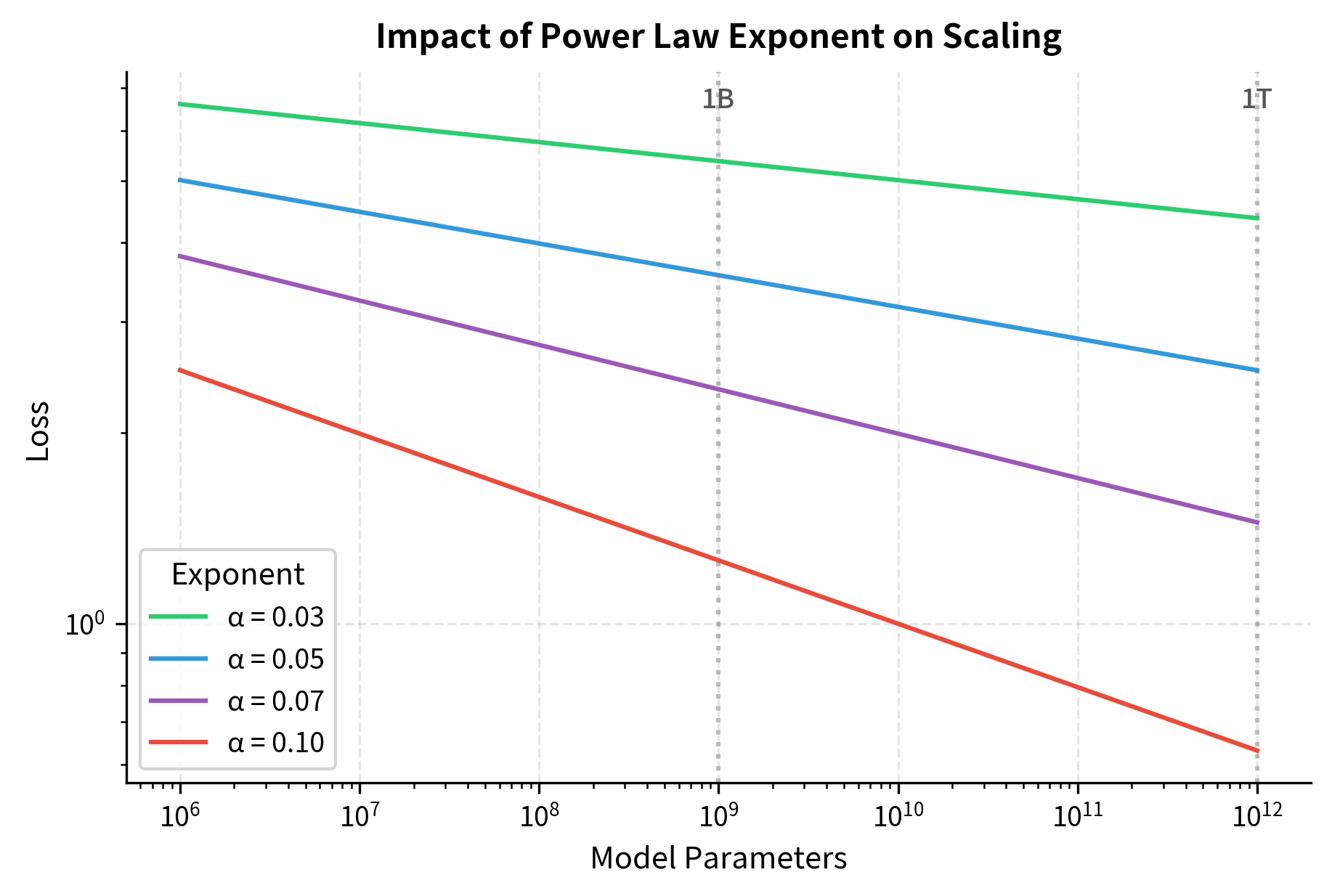
These numbers quantify the dramatic impact of the scaling exponent. With a modest exponent of 0.03, scaling by 100× yields only a 13% loss reduction, while an exponent of 0.10 delivers nearly three times the benefit at 37% reduction. The exponent makes an enormous difference. With $\alpha = 0.03$, going from 1B to 100B parameters (100×) reduces loss by about 13%. With $\alpha = 0.10$, the same scale-up reduces loss by about 37%. Understanding your specific power law exponent is crucial for efficient resource allocation.

The following visualization shows how these exponent differences compound over multiple orders of magnitude of scaling:

When applying power law analysis to real neural network scaling data, several practical issues arise that theory alone doesn't address. Being aware of these issues helps you avoid common pitfalls and interpret results appropriately.

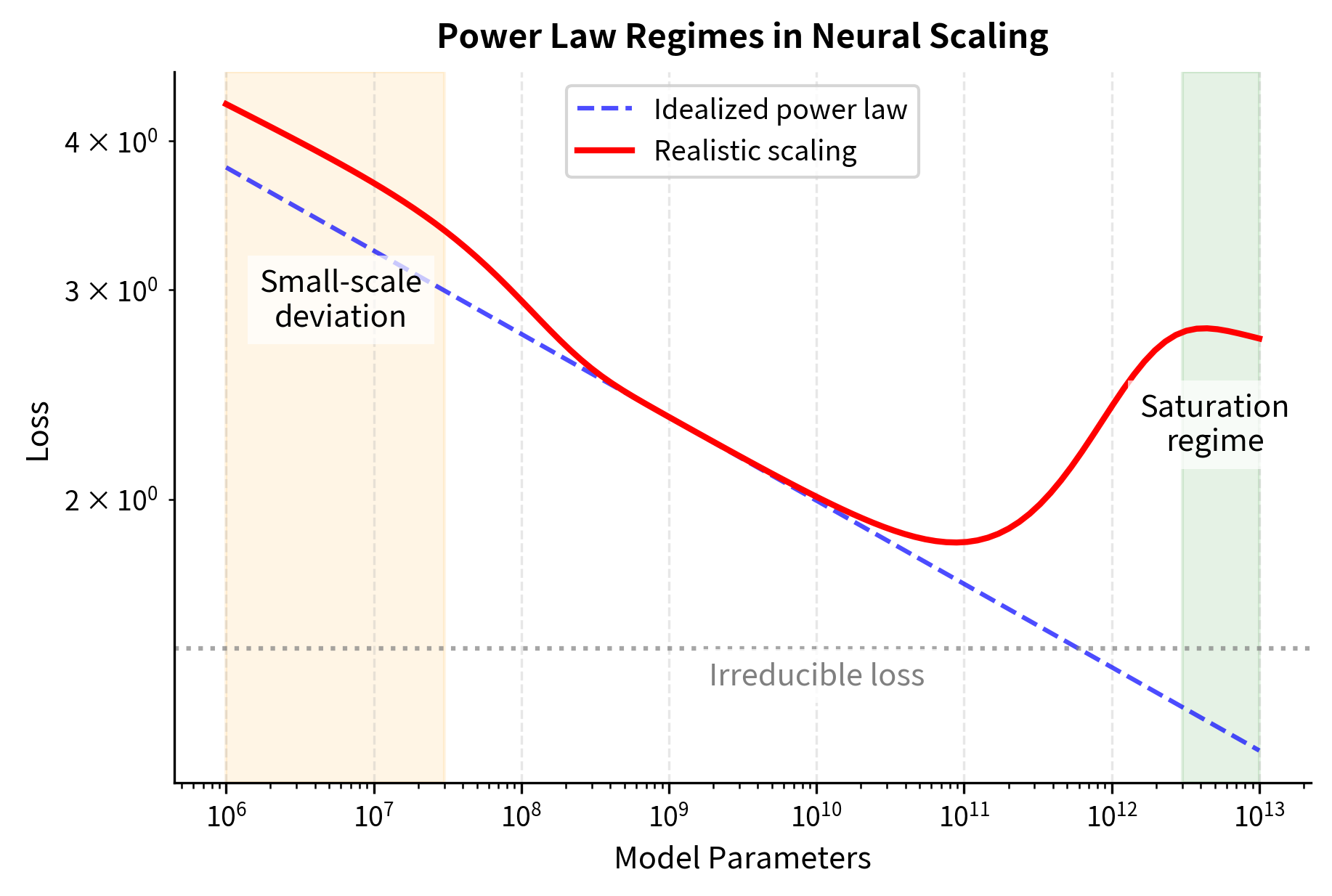
Finite-size effects. Very small models may not follow the same power law as larger ones. There is often a "small-model regime" where performance is worse than the power law predicts. This makes sense intuitively. A model with 100 parameters cannot possibly learn the complex patterns that a transformer needs, regardless of what the power law formula suggests. The power law describes behavior in a regime where the model has enough capacity to actually engage in meaningful learning.

Saturation at large scales. Power laws can't continue forever. Eventually, models approach irreducible limits such as noise in the data, task ambiguity, or the entropy of the underlying distribution. The power law form may break down at the frontier. If the true labels in your dataset have inherent randomness, such as annotator disagreement or ambiguous examples, no model can achieve zero loss. There is a floor below which you cannot go.

Multiple regimes. Some relationships show different power law exponents in different regions. For example, parameter scaling might have one exponent below 1B parameters and another above. These regime changes can correspond to qualitative shifts in what the model is learning, and fitting a single power law across multiple regimes produces misleading estimates.

Correlations between variables. Model size, data size, and compute are often increased together. Separating their individual contributions therefore requires careful experimental design. If you always double your data when you double your parameters, you cannot determine whether improvements come from more parameters, more data, or both. Controlled experiments that vary one factor while holding others constant are essential for understanding individual contributions.

These deviations don't invalidate power law analysis. Instead, they inform its proper use. Power laws describe intermediate regimes well but should be applied cautiously at extremes.

Power laws provide remarkably accurate descriptions of neural network scaling, but they have important limitations. First, they describe what happens but not why. A power law fit tells you the exponent but not the underlying mechanism producing it. Two completely different processes can yield identical power laws.

Second, power laws offer no guidance on optimal allocation. Knowing that loss decreases as $N^{-0.07}$ with parameters tells you how much improvement to expect from scaling, but not whether you should spend your compute budget on more parameters versus more training data. That question, which we'll address in the Chinchilla scaling laws chapter, requires understanding how multiple power laws interact.

Third, extrapolation carries risk. Power laws fit within the observed range can break down outside it. The successes of scaling predictions, such as researchers accurately forecasting GPT-4's performance from smaller experiments, should not obscure the fundamental uncertainty in extrapolating across orders of magnitude.

Despite these limitations, power laws have changed how the field approaches large-scale training. Before scaling laws were understood empirically, large training runs were expensive experiments with uncertain outcomes. Now, teams can run small-scale experiments to estimate scaling exponents, then predict with reasonable confidence how larger models will perform. This enables:

• Rational compute allocation decisions
• Risk assessment for large training investments
• Architecture comparison at equivalent compute
• Understanding of fundamental capability limits

The next chapters build on this foundation. We'll examine the specific scaling laws discovered by Kaplan et al. and later revised by Hoffmann et al. (Chinchilla), exploring how these power law relationships translate into practical training decisions.

Power laws describe relationships where one quantity varies as a power of another: $y = ax^b$. These relationships appear ubiquitously in deep learning, governing how model performance scales with parameters, data, and compute.

The key insights from this chapter are:

• Log-log linearity: Power laws become linear when plotted on logarithmic axes, making them easy to identify and fit.
• Scale invariance: The proportional change in output for a given proportional change in input is constant, regardless of absolute scale.
• Parameter estimation: Simple linear regression in log space recovers power law coefficients, enabling prediction beyond observed ranges.
• Universality: Power laws appear consistently across architectures, tasks, and resource types, suggesting deep connections to how neural networks learn.
• Practical intuition: Power laws mean diminishing but persistent returns. Orders of magnitude matter more than absolute quantities. Exponents determine scaling efficiency.

This mathematical framework provides the foundation for understanding the empirical scaling laws that have reshaped how we train large language models. In the next chapter, we'll examine the Kaplan scaling laws, which first quantified these relationships for transformer language models.

Ready to test your understanding? Take this quick quiz to reinforce what you've learned about power laws in deep learning.