

Master compute-optimal LLM training using Chinchilla scaling laws. Learn the 20:1 token ratio, practical allocation formulas, and training recipes for any scale.

This article is part of the free-to-read Language AI Handbook
Choose your expertise level to adjust how many terms are explained. Beginners see more tooltips, experts see fewer to maintain reading flow. Hover over underlined terms for instant definitions.
Compute-Optimal Training
Scaling laws reveal the fundamental relationships between compute, parameters, and data. But knowing these relationships is only the first step. The practical question every training run must answer is: given a fixed compute budget, how should I allocate resources between model size and training tokens?
As we discussed in the Chinchilla Scaling Laws chapter, Hoffmann et al. demonstrated that earlier approaches from Kaplan et al. significantly underestimated the importance of training data. Chinchilla showed that compute-optimal training requires balancing model size and training tokens in roughly equal proportions. This chapter translates those theoretical findings into actionable guidelines for planning and executing training runs.
We'll derive the formulas for optimal resource allocation, work through concrete examples of budget planning, examine how training hyperparameters interact with compute efficiency, and establish practical recipes that practitioners can apply directly. By the end, you'll understand not just what compute-optimal training means, but how to achieve it in practice.
The Compute Budget Problem
Training large language models is fundamentally a resource allocation problem that shares structural similarities with classical economics. Just as a business must decide how to allocate a fixed budget between labor and capital equipment, a machine learning practitioner must decide how to allocate a fixed compute budget between model capacity and training exposure. This decision is not just technical. It determines the fundamental character of the resulting model and shapes every downstream consideration from inference costs to capability profiles.
You have a fixed compute budget, typically measured in FLOPs (floating-point operations), and you must decide how to spend it. The two primary levers are:
- Model size (): More parameters mean more expressive capacity but also more FLOPs per training step
- Training tokens (): More data exposure improves learning but requires more total compute
Understanding why these two dimensions matter requires thinking about what actually happens during training. Model parameters represent the capacity of your neural network to store patterns, relationships, and abstractions learned from data. A larger model can represent more nuanced distinctions and capture longer-range dependencies. However, this capacity is merely potential. It must be actualized through exposure to training data. Training tokens represent the raw material from which the model extracts these patterns. Each token processed during training provides gradient signals that sculpt the parameter space, pushing the model toward configurations that predict text well.
The relationship between these quantities and total compute follows the approximation we established in earlier chapters:
where:
- : total compute in FLOPs (floating-point operations)
- : the number of non-embedding parameters in the model
- : the number of training tokens processed
- The factor of 6: accounts for approximately 2 FLOPs per parameter in the forward pass and 4 FLOPs per parameter in the backward pass (computing gradients and updating weights)
This formula deserves careful unpacking because it encapsulates a fundamental constraint. The factor of 6 arises from the computational structure of neural network training. During the forward pass, each parameter participates in roughly 2 floating-point operations (a multiply and an add for weighted sums). The backward pass requires computing gradients, which involves traversing the computational graph in reverse, costing approximately 2 more FLOPs per parameter. Finally, the optimizer update itself, when applying the gradient to modify weights, adds another 2 FLOPs per parameter. Together, these operations yield the factor of 6. This means that every token you process incurs a computational cost proportional to your model size, and every parameter you add increases the cost of processing every token.
Given this constraint, doubling your model size while keeping compute constant requires halving your training tokens. Conversely, doubling training tokens means using a smaller model. The question is: which allocation produces the best final model?
Why Equal Scaling Matters
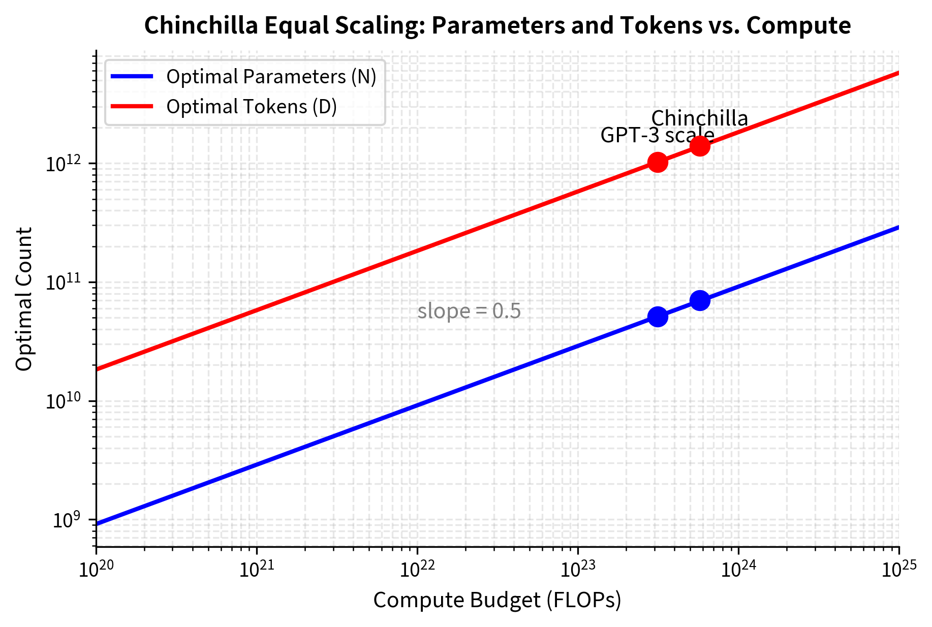
The Chinchilla findings established that compute-optimal training scales parameters and tokens equally with the compute budget. This result has important implications for how we think about model development. It tells us that neither model capacity nor data exposure is inherently more valuable; they are complements that must grow in tandem.
where:
- : the optimal number of model parameters for a given compute budget
- : the optimal number of training tokens for a given compute budget
- : the square root of compute, indicating both quantities scale with the same exponent
- : indicates proportionality (the quantities scale together, differing only by a constant factor)
The exponent of 0.5 appearing for both quantities is the mathematical signature of balanced scaling. To understand why this matters, consider what the square root implies operationally. When you increase your compute budget by a factor of 10, you should increase both model size and training tokens by a factor of . Neither dimension dominates, and both grow at the same rate.
This equal scaling arises from the structure of the loss function and how gradients balance across the two dimensions. Intuitively, think of model parameters and training data as two ingredients in a recipe. If you have abundant flour but little yeast, adding more flour will not improve your bread; you need more yeast. Similarly, if you have a massive model but limited training data, the model lacks the gradient signals needed to properly configure all those parameters. Conversely, if you have abundant data but a tiny model, the model lacks the capacity to absorb all the patterns present in the data. The equal scaling law tells us that these limitations bite at roughly the same rate, so optimal progress requires advancing both fronts simultaneously.
This result has important practical implications. Before Chinchilla, the prevailing wisdom based on Kaplan scaling suggested scaling models much faster than data. This led to models like Gopher (280B parameters, 300B tokens), which were significantly undertrained by Chinchilla standards. The compute spent on Gopher would have produced a better model at around 70B parameters trained on 1.4T tokens.
Optimal Allocation Formulas
Let's derive the formulas for compute-optimal training from first principles. This derivation illuminates the mathematical machinery behind the Chinchilla recommendations and provides insight into why the specific ratios emerge. Building on the Chinchilla loss function:
where:
- : the expected loss as a function of model size and data
- : the irreducible entropy of natural language (the theoretical minimum loss)
- : empirically fitted coefficients that determine the relative importance of model size vs. data
- : model parameters raised to power , capturing how loss decreases with model size
- : training tokens raised to power , capturing how loss decreases with more data
This functional form reveals important structure in language model training. The loss decomposes into three distinct components, each with a clear interpretation. The constant term represents the irreducible entropy of natural language, the inherent unpredictability that no model, however large or well-trained, can overcome. Human language contains genuine randomness: there are many ways to phrase the same idea, and even expert human predictions of the next word would not achieve zero error. The second term captures how loss decreases as you add model capacity. The power law form means that doubling your parameters doesn't halve this component of loss; rather, it reduces it by a factor of . The diminishing returns are already built into this formulation. Similarly, the third term captures how loss decreases with more training data, again with diminishing returns governed by the exponent .
The functional form reveals that loss decreases as power laws in both and , but with different exponents, meaning model size and data have different marginal returns. To find the optimal allocation given a fixed compute budget , we minimize loss subject to this constraint.
Using the method of Lagrange multipliers (or substitution), the optimal allocation satisfies:
where all variables are as defined above for the loss function. This implicit equation emerges from setting the partial derivatives of the Lagrangian to zero. The left side represents the ratio of parameters to tokens we seek to determine. The right side involves the empirical constants from the loss function, weighted by the ratio of exponents. The self-referential nature of this equation, where the ratio appears on both sides, reflects the coupled nature of the optimization problem. It can be solved by substituting the empirically fitted values (, , and the ratio ). After simplification, this yields a tokens-to-parameters ratio that Chinchilla estimated empirically:
This ratio tells us that for every parameter in your model, you should train on approximately 20 tokens. A 1B parameter model should see about 20B tokens, and a 70B model should see about 1.4T tokens.
This result is notable for its simplicity. Despite the complex optimization landscape and the many factors that could influence training, the optimal ratio distills to a single number that holds across orders of magnitude in compute scale. This ratio is remarkably stable across compute scales. Whether you're training a 1B or 100B parameter model, compute-optimal training uses approximately 20 tokens per parameter.
To develop intuition for why 20 tokens per parameter is the magic number, consider what happens at the extremes. If you train with far fewer tokens per parameter (say 2), your model has enormous capacity relative to the training signal it receives. Many parameters will be undertrained, effectively storing noise rather than useful patterns. The model might memorize training examples rather than learning generalizable features. Conversely, if you train with far more tokens per parameter (say 200), you're repeatedly refining a model that has already extracted most of what it can from the data given its limited capacity. The marginal improvement from each additional token becomes negligible. The ratio of 20 represents the sweet spot where both forms of inefficiency are minimized.
Practical Formulas
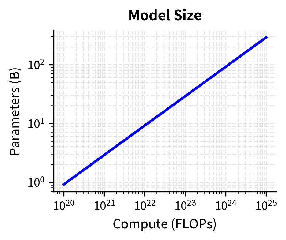
Given a compute budget (in FLOPs), the compute-optimal model size and token count are:
These formulas follow from combining with . Substituting the second into the first gives , which we solve for . This algebra transforms the abstract scaling principles into concrete, calculator-ready equations. The factor of 120 in the denominator encapsulates both the computational cost structure (the 6) and the optimal data ratio (the 20), bundling all the Chinchilla insights into a single coefficient.
For back-of-the-envelope calculations, these can be approximated as:
where:
- : the optimal number of model parameters
- : the optimal number of training tokens
- : total compute budget in FLOPs
- : derived from solving for
- : the token coefficient, since
These numerical coefficients make the formulas immediately usable. Given any compute budget expressed in FLOPs, you can quickly estimate the optimal allocation by taking the square root and scaling. The coefficient 0.091 for parameters is conveniently close to 0.1, making mental math tractable: a budget of FLOPs suggests optimal parameters around , or roughly 10 billion parameters.
Let's implement these formulas:
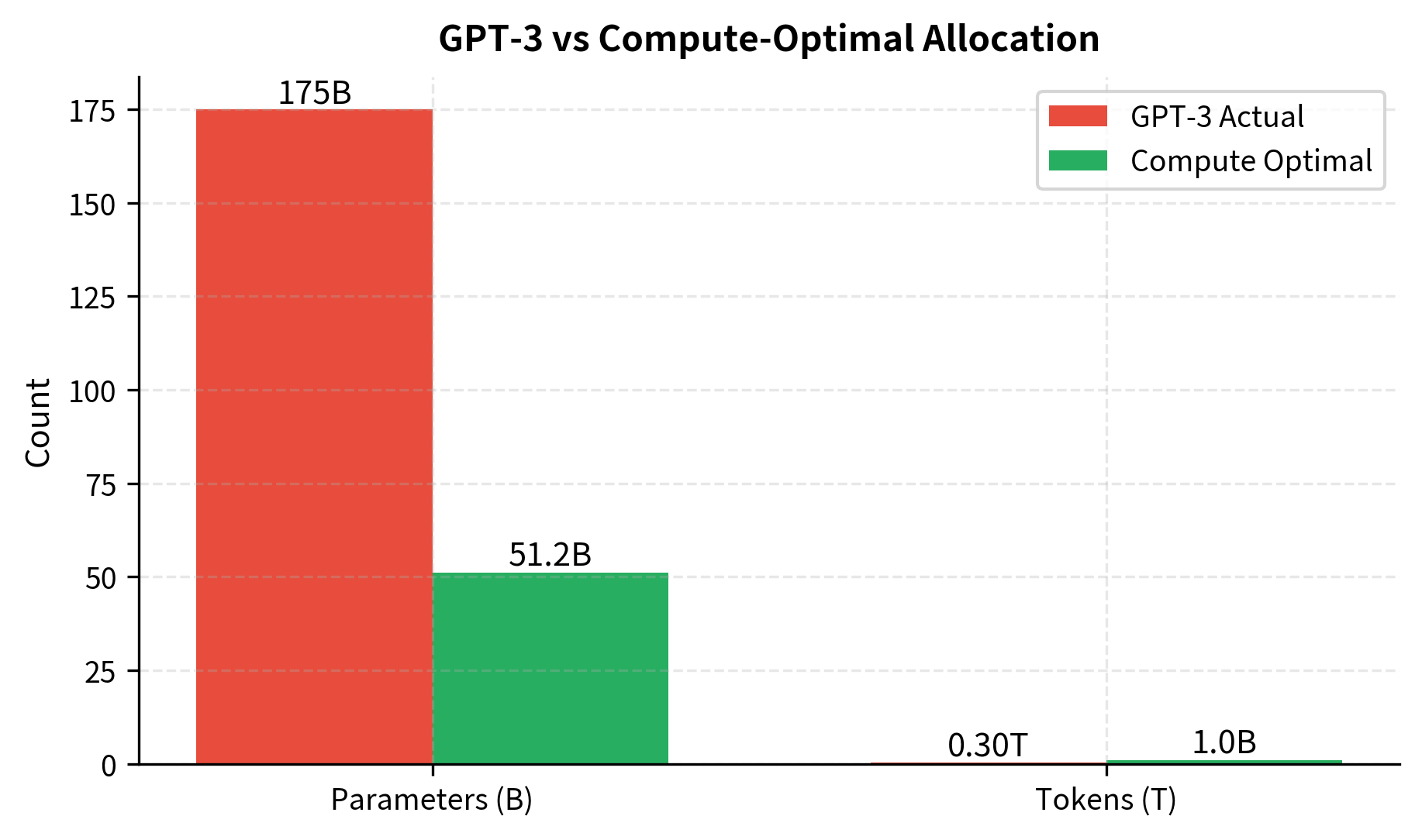
This calculation reveals that GPT-3 was significantly undertrained by Chinchilla standards. The comparison is striking: GPT-3 used only 1.7 tokens per parameter, roughly ten times less than the Chinchilla-optimal 20. This means the vast majority of GPT-3's 175 billion parameters were receiving insufficient training signal, they contributed to computational cost without being properly configured by data. The same compute budget would have produced a better model with around 51B parameters trained on over 1T tokens. This is essentially what Chinchilla demonstrated: their 70B model (trained on 1.4T tokens) outperformed the 280B Gopher despite using comparable compute.
Worked Example: Planning a Training Run
Let's walk through a complete example of planning a compute-optimal training run. This exercise illustrates how the theoretical formulas translate into concrete engineering decisions and demonstrates the cascade of choices that flow from the initial compute budget. Suppose you have access to a cluster with the following specifications:
- 128 A100 GPUs (80GB each)
- 2 weeks of dedicated training time
- Need to decide on model architecture and data requirements
Step 1: Calculate Available Compute
First, we estimate the total FLOPs available. This calculation bridges the gap between hardware specifications and the abstract compute budget that appears in our formulas. Understanding this translation is essential because hardware specifications are typically given in theoretical peak performance, while practical training achieves only a fraction of this peak:
Step 2: Determine Optimal Allocation
With our compute budget established, we can now apply the Chinchilla formulas to determine how that compute should be allocated. This step converts an abstract resource constraint into concrete targets for model size and data requirements:
Step 3: Choose Architecture
The optimal parameter count guides architecture selection. However, parameter count alone does not determine architecture, there are many ways to arrange 2.2 billion parameters. The key architectural decisions involve the tradeoff between depth (number of layers) and width (hidden dimension), along with choices about attention heads, feed-forward dimensions, and normalization strategies. For a ~2.2B parameter model, we need to choose depth (layers), width (hidden dimension), and other hyperparameters:
Step 4: Plan Data Pipeline
The optimal token count determines data requirements. This step connects the abstract token count to the concrete challenge of sourcing, processing, and storing training data. The gap between "we need 44 billion tokens" and "we have these specific datasets available" requires careful planning:
This planning process shows how compute-optimal allocation drives downstream decisions about architecture and data sourcing. The cascade from compute budget to model size to architecture to data requirements illustrates why compute-optimal thinking must inform the entire planning process, not just final training decisions.
Training Efficiency in Practice
Compute-optimal formulas assume you extract maximum value from each FLOP. In practice, many factors affect training efficiency, and optimizing these factors can significantly impact your effective compute budget. The gap between theoretical compute (what the formulas predict) and practical compute (what you actually achieve) can be substantial. Understanding this gap is essential for realistic planning and for identifying opportunities to improve training efficiency.
Model FLOPs Utilization
Model FLOPs Utilization (MFU) measures what fraction of theoretical peak hardware performance you actually achieve. This metric captures the cumulative effect of all inefficiencies in a training system, from memory bandwidth bottlenecks to communication overhead to operations that cannot fully utilize specialized hardware:
where:
- : Model FLOPs Utilization, a ratio between 0 and 1 (often expressed as a percentage)
- : the actual floating-point operations per second achieved during training
- : the theoretical maximum operations per second the hardware can perform
For example, an A100 GPU has a peak of 312 TFLOPS for FP16 tensor operations. If your training achieves 140 TFLOPS of actual compute, your MFU is . The gap comes from memory bandwidth limitations, communication overhead, and operations that cannot fully utilize tensor cores. This 55% gap might seem wasteful, but it reflects real constraints. Moving data between GPU memory and compute units takes time; synchronizing gradients across GPUs requires communication; and not every operation in a transformer maps efficiently onto tensor cores.
Typical MFU values for LLM training range from 30% to 60%, depending on:
- Hardware configuration: Multi-GPU communication overhead reduces MFU as cluster size grows
- Batch size: Larger batches amortize fixed costs but may require more memory
- Model architecture: Some operations (LayerNorm, activations) are memory-bound rather than compute-bound
- Precision: Mixed precision training (FP16/BF16 with FP32 accumulation) typically achieves higher MFU than FP32
Each of these factors represents an engineering challenge with its own optimization strategies. Hardware communication overhead can be reduced through careful placement of operations, overlapping communication with computation, and using efficient collective primitives. Batch size choices involve tradeoffs between memory pressure, gradient quality, and throughput. Architecture decisions affect the ratio of compute-bound to memory-bound operations, with implications for how efficiently the hardware can be utilized.
A 30% improvement in MFU (from 30% to 60%) cuts training time in half. This makes MFU optimization a critical concern for compute-optimal training. The practical implication is that engineering effort invested in improving MFU pays dividends equivalent to acquiring additional hardware. Improving MFU from 30% to 60% is equivalent to doubling your GPU count at no additional hardware cost.
Learning Rate Schedules
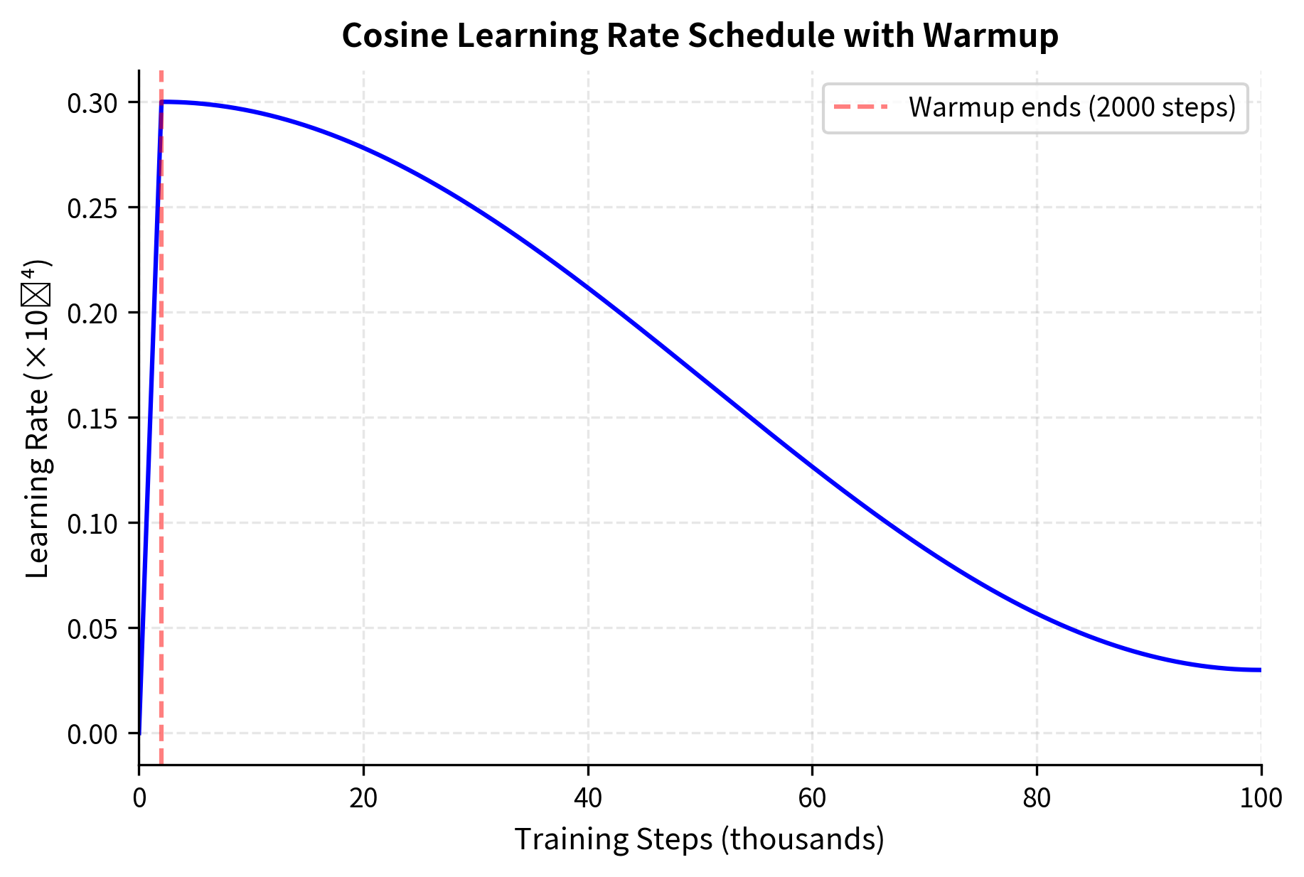
Learning rate scheduling significantly affects training efficiency. The learning rate controls how aggressively the optimizer updates model parameters in response to gradient signals. Too high, and training becomes unstable as updates overshoot optimal parameter values. Too low, and training proceeds sluggishly, wasting compute on inefficient updates. The standard approach for LLM training uses:
- Warmup: Linear increase from near-zero to peak learning rate
- Decay: Cosine or linear decay to a minimum value
The warmup phase serves a critical stability function. At initialization, model parameters are random and gradients can be unreliable. Large learning rates applied to noisy gradients cause training to diverge. By starting with small learning rates and gradually increasing, warmup allows the model to find a stable region of the loss landscape before aggressive optimization begins. The decay phase addresses a different concern: as training progresses and the model approaches a good solution, large learning rates cause the optimizer to overshoot and oscillate around the minimum. Gradually reducing the learning rate allows fine-grained convergence.
The key parameters are:
- Peak learning rate: Scales inversely with model size; larger models use smaller learning rates
- Warmup steps: Typically 0.1% to 1% of total training steps
- Minimum learning rate: Usually 10% of peak, though some schedules decay to zero
Batch Size Scaling
Batch size affects both training dynamics and compute efficiency. Understanding batch size requires recognizing that gradient descent operates on estimated gradients. Each batch provides a noisy estimate of the true gradient, with larger batches providing more accurate estimates at the cost of more computation per update. The critical batch size is the point beyond which larger batches provide diminishing returns. Below this threshold, doubling batch size nearly halves training time. Above it, larger batches waste compute on redundant gradient information.
The diminishing returns arise from the statistical nature of gradient estimation. With small batches, each sample contributes significant independent information about the gradient direction. As batch size grows, samples begin to provide redundant information, they agree on the gradient direction, so averaging more of them improves the estimate only marginally. The critical batch size marks the transition between these regimes.
Empirically, the critical batch size scales with loss. As training progresses, the gradient signal becomes noisier relative to its magnitude, meaning that averaging over more samples (larger batches) provides diminishing returns. The relationship is:
where:
- : the critical batch size, beyond which larger batches provide diminishing returns
- : the inverse of the current loss value
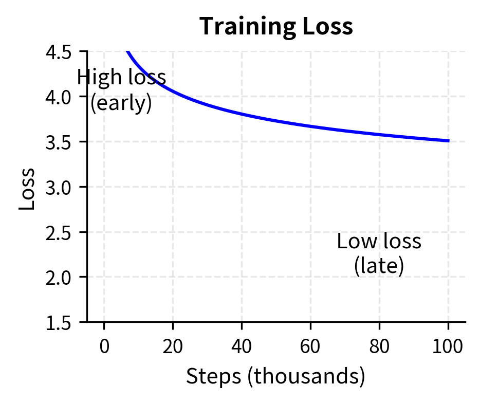
This inverse relationship has an intuitive explanation: when loss is high (early in training), gradients are large and consistent across samples, so even small batches provide reliable gradient estimates. As loss decreases and the model approaches convergence, gradients become smaller and noisier, requiring more samples to average out the noise and get a reliable signal. This is why early in training (when loss is high), smaller batches are optimal. As the model improves and loss drops, it can benefit from larger batches.
Think of it this way: early in training, the model is making large, obvious mistakes that any sample can reveal. A small batch suffices to identify that "the model thinks 'the' should follow 'the', and that's wrong." Later in training, the model's errors are subtle, and any individual sample might push the gradient in a misleading direction due to noise. Larger batches average out these idiosyncratic signals to reveal the true underlying gradient.
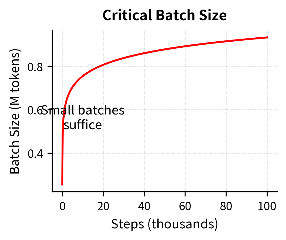
As training progresses and loss decreases, the critical batch size increases. This motivates batch size warmup strategies that start with smaller batches and gradually increase throughout training.
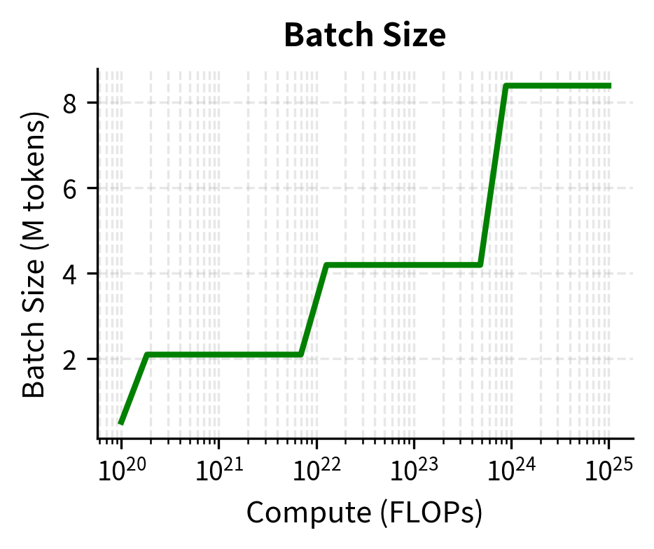
For compute-optimal training, practitioners typically:
- Start with batch sizes of 256K to 1M tokens
- Increase batch size 2-4x during training if the schedule allows
- Use gradient accumulation to achieve large effective batch sizes on limited hardware
Compute-Optimal Recipes
Based on scaling laws and practical experience, we can establish concrete recipes for different compute scales. These recipes synthesize insights from Chinchilla and subsequent work to provide starting points for training runs. They represent practical wisdom distilled from experience, not rigid prescriptions. Each recipe encodes decisions about architecture, hyperparameters, and training procedures that have been validated across many training runs.
Small-Scale Training (10^20 - 10^21 FLOPs)
This regime corresponds to models in the 100M to 1B parameter range, trainable on a single node of 8 GPUs in days to weeks. These scales are accessible to academic researchers and small teams, making them important proving grounds for new techniques.
The key recommendations are:
- Architecture: 12-24 layers, 768-2048 hidden dimension
- Tokens: 2-20B tokens (maintaining 20:1 token-to-parameter ratio)
- Learning rate: 3e-4 to 6e-4 peak
- Batch size: 256K to 512K tokens
- Warmup: 1% of total steps
Medium-Scale Training (10^22 - 10^23 FLOPs)
This regime covers models from 3B to 30B parameters, requiring multi-node training over weeks. These scales represent the domain of well-resourced research labs and enterprise training efforts. The engineering challenges shift from single-machine optimization to distributed systems coordination.
The key recommendations are:
- Architecture: 32-48 layers, 3072-5120 hidden dimension
- Tokens: 60B-600B tokens
- Learning rate: 1.5e-4 to 3e-4 peak
- Batch size: 1M to 4M tokens
- Warmup: 0.5% of total steps
- Parallelism: Tensor parallelism across 4-8 GPUs, data parallelism across nodes
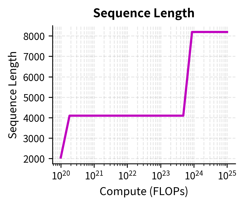
Large-Scale Training (10^24+ FLOPs)
For frontier models (70B+ parameters), compute-optimal training requires careful attention to factors that become critical only at extreme scale. Training runs at this scale can take months, making each decision consequential and recovery from errors expensive.
The key considerations are:
- Extended context: Longer sequences (4K-32K tokens) for quality
- Data quality: Heavy filtering and deduplication become essential
- Checkpoint strategy: Frequent saves due to long training times
- Gradient checkpointing: Trade compute for memory to fit larger models

Beyond Compute Optimality
Compute-optimal allocation minimizes loss for a fixed compute budget, but this is not always the right objective. Several scenarios call for deviating from the Chinchilla ratio. Understanding when and why to deviate requires looking beyond "minimize validation loss given training compute" to consider the full lifecycle of a model.
Inference Constraints
If your model will serve many inference requests, a smaller, longer-trained model may be preferable. The extra training compute is a one-time cost, while inference compute accumulates over the model's lifetime. This asymmetry changes the optimization problem significantly.
Consider a model that will process 1 trillion tokens during deployment. The total lifetime compute is:
where:
- : total compute over the model's lifetime (training plus inference)
- : training compute (forward and backward passes)
- : inference compute (forward passes only, hence factor of 2 not 6)
- : total tokens processed during inference deployment
The factor of 2 for inference (vs. 6 for training) reflects that inference only requires forward passes. During training, we compute the forward pass, then the backward pass for gradients, then apply optimizer updates. During inference, we only need the forward pass to generate predictions. This is why inference-heavy applications favor smaller, over-trained models. When is large, the optimal training allocation shifts toward smaller models.
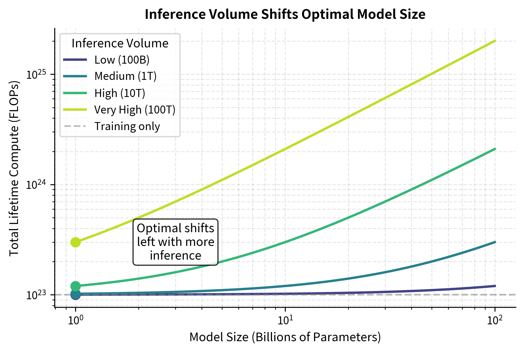
The implication is clear: for a model that will serve billions of inference requests, the optimal strategy may be to train a model that is two or three times smaller than the Chinchilla-optimal size, but train it on correspondingly more data. This "inference-optimal" model will have slightly higher loss than a Chinchilla-optimal model trained with the same compute, but the total lifetime cost (training plus inference) will be lower.
This reasoning led to models like LLaMA 2, which was 7B parameters trained on 2T tokens (286 tokens per parameter), intentionally "over-trained" by Chinchilla standards but more efficient at inference.
Data Constraints
When high-quality training data is limited, you may not have enough tokens to train a compute-optimal model. In this case, you face a choice:
- Train a smaller model on available data (staying near 20:1 ratio)
- Train the larger model with data repetition (exceeding 1 epoch)
- Invest in data augmentation or synthetic data generation
We'll explore these tradeoffs in detail in the upcoming chapter on Data-Constrained Scaling.
Capability Thresholds
Some capabilities emerge only above certain model sizes, as we'll discuss in Part XXII on Emergence. If your application requires a capability that emerges at 10B parameters, a compute-optimal 3B model will not suffice regardless of how much data you train on.
In such cases, the strategy is to train an undertrained larger model that crosses the capability threshold, then potentially continue training or fine-tune on domain-specific data.
Limitations and Impact
Compute-optimal training changed how the field approaches model development. Before Chinchilla, the assumption was that bigger models were always better, leading to parameter counts that outpaced training data. The 20:1 tokens-to-parameters guideline provided a concrete, actionable target and redirected industry investment toward data curation and extended training.
However, the Chinchilla ratio has important limitations. The original analysis focused on validation loss as the optimization target, which does not correlate perfectly with downstream task performance. Some capabilities may require different scaling behaviors than raw perplexity improvement. The 20:1 ratio also assumes specific hyperparameter choices (learning rate schedules, batch sizes) and may not hold for significantly different training setups.
The ratio also emerged from training on English-dominated web text. Different data distributions, such as multilingual corpora, code, or scientific literature, may have different optimal allocation curves. Recent work has shown that heavily filtered data enables more efficient training, potentially shifting the optimal ratio toward even more tokens per parameter.
Perhaps most importantly, compute-optimal training optimizes for a single training run. In practice, organizations may prefer smaller models that enable faster iteration, easier deployment, and lower inference costs. The "optimal" allocation depends on the full lifecycle cost, not just training compute.
Despite these caveats, the Chinchilla framework provides useful guardrails. Training a 100B model on 100B tokens is clearly wasteful; training a 1B model on 200B tokens likely hits diminishing returns. The 20:1 ratio gives practitioners a well-calibrated starting point from which to make informed deviations based on their specific constraints.
Summary
This chapter translated scaling laws into practical training recipes. The key takeaways are:
- Compute-optimal allocation balances model size and training tokens according to , where both scale as with compute budget
- Planning a training run involves calculating total FLOPs, deriving optimal parameter and token counts, selecting an architecture, and sizing the data pipeline accordingly
- Training efficiency depends critically on Model FLOPs Utilization, which varies from 30-60% depending on hardware configuration, batch size, and implementation quality
- Hyperparameters scale with model size: larger models use smaller learning rates, larger batch sizes, and longer sequences
- Practical recipes vary by scale, from single-node runs at 10^21 FLOPs to distributed training at 10^24 FLOPs and beyond
- Deviation from optimality is appropriate when inference costs dominate, data is constrained, or capability thresholds matter more than raw loss
The next chapter on Data-Constrained Scaling explores what happens when you can't reach the optimal token count, examining strategies for training under data limitations and the effectiveness of data repetition.
Key Parameters
The key parameters for compute-optimal training are:
- tokens_per_param: The optimal ratio of training tokens to model parameters, approximately 20 for Chinchilla-optimal training.
- compute_flops: Total compute budget in floating-point operations, determining the scale of training.
- mfu (Model FLOPs Utilization): Fraction of theoretical peak hardware performance achieved during training, typically 30-60%.
- peak_lr: Maximum learning rate during training, scaling inversely with model size.
- warmup_steps: Number of steps for linear learning rate warmup, typically 0.5-1% of total steps.
- batch_tokens: Number of tokens per batch, scaling with model size from 256K to 8M tokens.
Quiz
Ready to test your understanding? Take this quick quiz to reinforce what you've learned about compute-optimal training and resource allocation.

Comments