KV Cache Explained: Efficient Attention for LLM Generation

When you ask a language model to complete the sentence "The capital of France is," it generates tokens one at a time: first "Paris," then perhaps a comma, then additional context. At each step, the model computes attention over all previous tokens to decide what comes next. Without optimization, this means the model recomputes the same attention calculations for "The," "capital," "of," "France," "is" every single time it generates a new token. For a 100-token response, that's nearly 5,000 redundant computations just for the prompt tokens.

The key-value cache, commonly called KV cache, eliminates this redundancy by storing the intermediate attention computations and reusing them across generation steps. This optimization reduces the complexity of autoregressive generation from quadratic to linear, making inference with large language models feasible.

As we explored in Part XVIII, decoder-only transformers generate text one token at a time. At each step, the model takes all tokens generated so far (including the prompt) and predicts the next token. The computational core of this process is the self-attention mechanism, which allows each token to gather information from all tokens that came before it. To understand why caching provides such dramatic benefits, we must first examine exactly how attention operates during generation and identify where the redundant work occurs.

Recall from Part X that self-attention computes queries, keys, and values from the input. The fundamental insight behind these three components is that attention works like an information retrieval system: queries represent what a token is looking for, keys represent what each token offers, and values contain the actual information to be retrieved. We can express this through three linear projections:

where:

• $X$: the input embedding matrix, containing the vector representations of all tokens in the sequence
• $W_Q, W_K, W_V$: the learned projection matrices that transform inputs into query, key, and value subspaces, each capturing a different aspect of the token's meaning
• $Q, K, V$: the resulting matrices, where Q contains vectors representing what each token seeks, K contains vectors representing what each token can be matched against, and V contains the actual content to be aggregated

Each of these projection matrices is learned during training to extract the most useful representations for the attention mechanism. Once training is complete, these matrices remain fixed during inference. This means that given the same input token, the projections will always produce the same key and value vectors, a property that forms the foundation for caching.

The attention mechanism then computes a weighted sum of values based on the compatibility between queries and keys. This compatibility is measured through dot products, which capture how well a query's "question" matches each key's "answer." The full attention formula is:

where:

• $Q, K, V$: the query, key, and value matrices computed from the input
• $K^T$: the transpose of the key matrix, arranged so that the dot product between queries and keys can be computed efficiently through matrix multiplication
• $d_k$: the dimension of the key vectors, used for scaling to prevent the dot products from growing too large and causing vanishing gradients in the softmax
• $\text{softmax}$: the function that converts raw compatibility scores into probability weights summing to 1, ensuring all weights are positive and amplifying differences so that tokens with higher compatibility receive substantially more attention

The scaling factor $\sqrt{d_k}$ is critical. Without this normalization, the dot products between high-dimensional vectors can become very large in magnitude. When these large values pass through the softmax function, the result becomes extremely peaked, meaning almost all attention weight concentrates on a single token. This causes gradients to vanish for all other positions, making training unstable. The square root scaling keeps the variance of the dot products roughly constant regardless of the dimension.

During generation, let's trace what happens at each step to understand precisely where redundancy arises. Suppose we're generating a response to a 10-token prompt. The model must produce one token at a time, with each new token depending on everything that came before it.

Step 1: The model processes all 10 prompt tokens simultaneously in what we call the prefill phase. It computes the $Q$, $K$, $V$ matrices, each of shape $(10, d_k)$ or $(10, d_v)$ depending on the specific projection. The attention mechanism then allows each prompt token to attend to all previous prompt tokens, establishing the initial context representation.

Step 2: After generating the first new token, we now have 11 tokens total. Without any optimization, the model would need to process the entire 11-token sequence from scratch. This means computing $Q$, $K$, $V$ for all 11 tokens, even though 10 of them are unchanged from the previous step.

Step 3: With 12 tokens total, we compute $Q$, $K$, $V$ for all 12 tokens, once again recomputing the projections for the original prompt tokens that haven't changed at all.

Notice the wasteful pattern emerging: at step $t$, we recompute the keys and values for the first 10 prompt tokens, even though nothing about them has changed since step 1. The same tokens, passing through the same fixed projection matrices $W_K$ and $W_V$, produce the same $K$ and $V$ vectors every single time. This redundancy stems from a fundamental property of the attention mechanism: the key and value for a given token depend only on that token's embedding and the projection weights, not on what comes after it in the sequence.

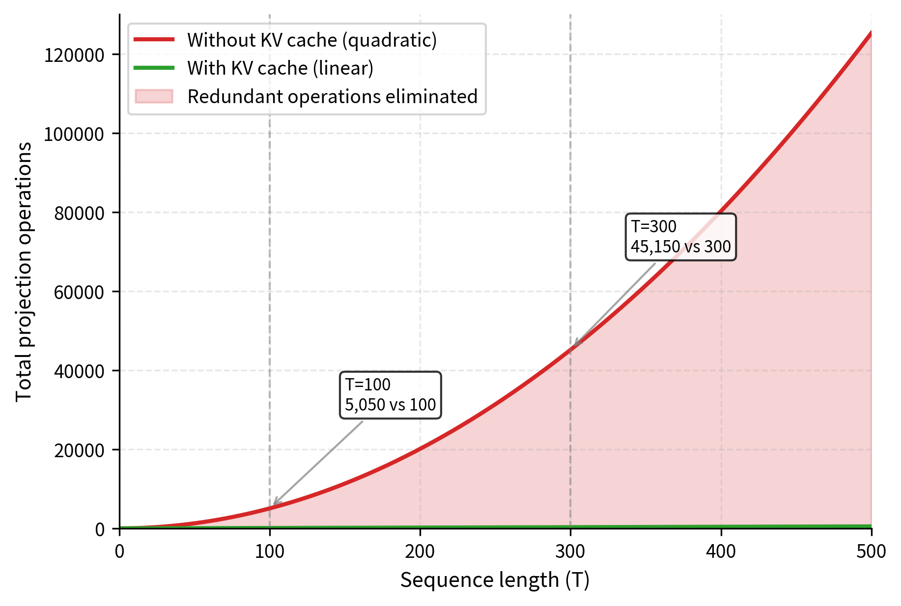
This redundancy has concrete costs that grow dramatically with sequence length. For a model with $L$ layers, $H$ attention heads, and head dimension $d_h$, generating $T$ tokens requires computing $K$ and $V$ projections repeatedly at every step. The total number of projection operations across all generation steps sums to:

where:

• $T$: the final sequence length, representing the total number of tokens processed including both the prompt and generated tokens
• $t$: the current step number, which also represents the sequence length at that particular step
• $\sum_{t=1}^{T} t$: the sum of the arithmetic progression $1 + 2 + 3 + \ldots + T$, capturing the total number of token-projection operations across all steps

This quadratic scaling has severe implications for practical deployment. If generating 100 tokens requires $\frac{100 \times 101}{2} = 5,050$ projection operations, then generating 1,000 tokens requires $\frac{1000 \times 1001}{2} = 500,500$ operations, a 100-fold increase in work for only a 10-fold increase in output length. This contrasts with the ideal case where each token's keys and values are computed only once, requiring $T$ projection operations. The KV cache achieves this by computing each projection once and storing it for future reuse.

The insight behind KV caching is straightforward once we recognize where the redundancy lies: since each token's key and value vectors depend only on that token's representation and the fixed projection weights, we can compute them once and store them for reuse in all subsequent generation steps. The query vectors, by contrast, must be recomputed because they are used differently at each step. A query asks "what information should I attend to?" and the answer depends on the token's position in the evolving sequence.

This asymmetry between queries and key-values is fundamental to understanding the cache. When token 5 generates a query, it needs to attend to tokens 1 through 4. When token 10 generates a query, it needs to attend to tokens 1 through 9. The keys and values for tokens 1 through 4 are the same in both cases, they haven't changed. But the query's role is different: it's always asking about everything that came before, and "everything that came before" grows with each step.

During generation with KV caching, the process changes fundamentally from the naive approach:

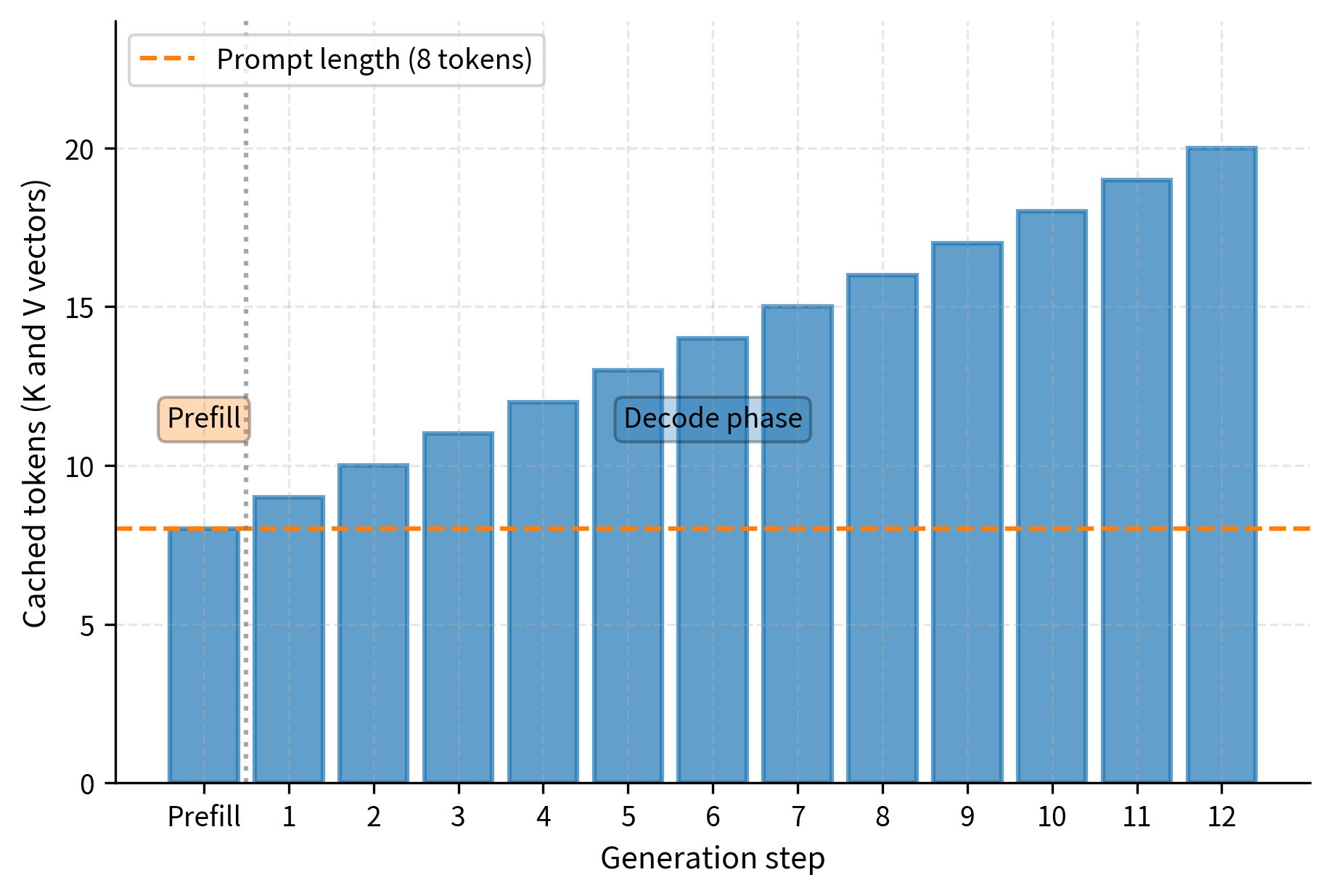
Prefill phase (Step 1): Process all prompt tokens at once, computing queries, keys, and values for the entire prompt. Store the computed $K$ and $V$ matrices in the cache, as these will be reused throughout generation. Use the queries to compute attention within the prompt, establishing the initial hidden states.

Decode phase (Steps 2+): For each new token, the process is efficient:

1. Compute $Q$, $K$, $V$ only for the single new token
2. Append the new $K$ and $V$ vectors to the end of the cache
3. Compute attention using the new $Q$ against all cached $K$ values
4. Weight all cached $V$ values by the resulting attention scores
5. Produce the output for this position

The crucial difference is that we only compute projections for one token per step (the newly generated one), while the attention computation can freely access all previously computed keys and values through the cache. This transforms the projection work from quadratic to linear in the total sequence length.

Let's formalize this caching mechanism to understand exactly how it achieves the computational savings. The formalization reveals that caching is not an approximation but an algebraically equivalent reformulation of the attention computation.

At generation step $t$, let $x_t$ denote the embedding of the newly generated token. This embedding captures all the information the model has about this token at the input to the attention layer. We project this single token's embedding to obtain its query, key, and value vectors:

where:

• $x_t$: the input embedding for the current token at step $t$, a vector of dimension $d_{\text{model}}$
• $W_Q, W_K, W_V$: the fixed projection matrices shared across all positions and all generation steps
• $q_t$: the query vector representing what the current token is seeking to attend to
• $k_t$: the key vector representing how this token can be matched by future queries
• $v_t$: the value vector containing the information this token contributes when attended to

Note the important distinction from the non-cached case: each of these is a single vector of dimension $d_k$ or $d_v$, not a full matrix covering all positions. We compute projections for exactly one token, not the entire sequence.

The cache serves as the model's memory of past tokens, maintaining the history of key and value vectors computed in all previous steps. At the beginning of step $t$, before processing the new token, the cache contains concatenated matrices:

where:

• $K_{\text{cache}}, V_{\text{cache}}$: matrices storing the complete history of keys and values for all previous $t-1$ tokens
• $k_i, v_i$: the key and value vectors computed when token $i$ was first processed
• $[;]$: the concatenation operation along the sequence dimension, stacking vectors as rows
• $d_k, d_v$: the dimensions of the key and value vectors, often equal in practice

This cache represents all the "memory" the attention mechanism has of the sequence so far. Each row corresponds to a token's contribution to the attention computation.

After computing the new token's projections, we update the cache by appending the new key and value vectors:

where:

• $K_{\text{cache}}, V_{\text{cache}}$: the cached key and value matrices being extended with new entries
• $\leftarrow$: the assignment operator indicating an in-place update to the stored cache state
• $k_t, v_t$: the newly computed key and value vectors being appended to preserve the sequence history

After this update, the cache contains keys and values for all $t$ tokens, ready for the attention computation.

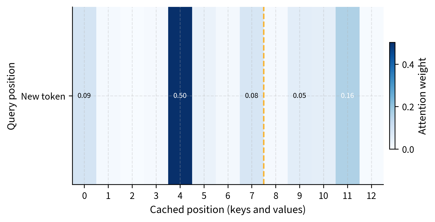
With the cache updated, the model computes attention for the new token by having its query vector interact with the entire history:

where:

• $a_t$: the attention weights for the current step, a vector of $t$ probabilities representing how much the new token should attend to each previous position
• $q_t$: the query vector for the current token, seeking relevant information from the context
• $K_{\text{cache}}^T$: the transpose of the cached key matrix, shaped for efficient dot product computation with the query
• $V_{\text{cache}}$: the cached value matrix containing the actual content to be retrieved and aggregated
• $d_k$: the dimension of key vectors, providing the scaling factor for numerical stability
• $d_v$: the dimension of value vectors, determining the output size
• $o_t$: the final attention output for step $t$, a weighted combination of all cached values

The computation $q_t K_{\text{cache}}^T$ produces a vector of $t$ scores, one for each cached position. These scores measure how relevant each previous token is to the current query. After scaling and applying softmax, these become proper attention weights that sum to 1. Finally, multiplying by $V_{\text{cache}}$ aggregates the cached values according to these weights, producing the output vector that captures all the relevant information from the sequence history.

This formulation achieves efficiency because the matrix multiplications involve a single query vector against the cached matrices, requiring $O(t \times d)$ operations rather than $O(t^2 \times d)$ that would be needed to recompute attention from scratch.

The KV cache must be maintained separately for each layer and each attention head in the transformer architecture. This requirement arises because different layers and heads learn different attention patterns and have different projection weights. Layer 1's keys and values are fundamentally different from layer 32's, as each layer captures different levels of abstraction. Similarly, within a layer, head 1 might learn to track syntactic relationships while head 4 tracks semantic similarity, each requiring its own separate cache.

For a transformer with $L$ layers and $H$ attention heads per layer, the complete cache consists of $2 \times L \times H$ tensors: one $K$ cache and one $V$ cache for each attention head at each layer. This combinatorial structure means that even modest models require tracking many separate cache tensors.

In practice, deep learning frameworks typically consolidate this organization into two tensors per layer, using an additional dimension to index across heads:

where:

• $K_{\text{cache}}^{(l)}, V_{\text{cache}}^{(l)}$: the key and value cache tensors for layer $l$, containing caches for all heads
• $B$: the batch size, allowing multiple sequences to be processed in parallel
• $H$: the number of attention heads, each with its own cached key-value pairs
• $T$: the current sequence length, growing as generation proceeds
• $d_h$: the head dimension, typically $d_{\text{model}} / H$

Some implementations combine keys and values into a single tensor of shape $(B, H, T, 2, d_h)$ or $(B, 2, H, T, d_h)$ for improved memory locality. This layout keeps each position's key and value adjacent in memory, which can improve cache efficiency during the attention computation. However, the logical structure remains the same regardless of the physical memory layout.

Understanding how the cache integrates with the transformer's layer-by-layer computation clarifies why the optimization is both correct and efficient. During the decode phase, when generating token by token, each transformer layer performs the following sequence of operations:

1. Receives the hidden state for only the new token: $h_t^{(l)} \in \mathbb{R}^{B \times 1 \times d_{\text{model}}}$. This is the representation of the new token as computed by the previous layer.
2. Projects this hidden state to obtain $q_t$, $k_t$, $v_t$ for the new token only.
3. Retrieves the cached $K_{\text{cache}}^{(l)}$ and $V_{\text{cache}}^{(l)}$ containing all previously computed keys and values for this layer.
4. Appends the new $k_t$ and $v_t$ to the cache, extending the history by one position.
5. Computes attention between the new query $q_t$ and the full cache, allowing the new token to attend to all previous positions.
6. Passes the attention output through the feed-forward network, which processes each position independently.
7. Returns the hidden state for the new token: $h_t^{(l+1)}$, ready for the next layer.

Notice that operations 1, 2, 6, and 7 all operate on just a single position. The feed-forward network, layer normalization, and residual connections process only the new token's hidden state, making them computationally trivial during decoding. The attention computation in step 5 is the only operation that touches the full sequence length, and even there, the work is linear in $t$ rather than quadratic because we compute attention for just one query position.

Understanding KV cache memory consumption is essential for deployment planning, as the cache often becomes the primary memory bottleneck in production systems. Unlike model weights that have a fixed size, the cache grows dynamically during generation and can easily exceed the model weights in memory usage for long sequences or large batches.

To derive the memory requirements, we must account for all the tensors that constitute the complete cache. For a single sequence of length $T$, we need to store keys and values for every layer and every head. The fundamental memory formula is:

where:

• $2$: accounts for storing both keys and values, as each requires a separate tensor
• $L$: the number of transformer layers, each maintaining its own independent cache
• $H$: the number of attention heads per layer
• $d_h$: the dimension of each head, determining the size of individual key and value vectors
• $T$: the sequence length in tokens, the dynamic factor that grows during generation
• $\text{bytes per element}$: the memory size required for a single floating-point number (e.g., 2 bytes for FP16, 4 bytes for FP32)

Since the total model dimension is typically expressed as $d_{\text{model}} = H \times d_h$, we can simplify this formula by substituting:

where:

• $d_{\text{model}}$: the total model dimension, equal to $H \times d_h$
• $L$: the number of layers in the model
• $T$: the sequence length
• $\text{bytes per element}$: the numerical precision in bytes

This simplified formula reveals an important insight: the cache memory scales with the product of model depth and width, multiplied by sequence length. Doubling any of these factors doubles the memory requirement.

To make these formulas concrete, let's calculate the cache requirements for a widely deployed model. The LLaMA 2 7B model has the following specifications:

• $L = 32$ layers
• $d_{\text{model}} = 4096$
• Typically stored in FP16 (2 bytes per element)

For a single sequence of length $T = 2048$, we can compute the cache size step by step:

A single 2048-token sequence requires a full gigabyte just for the KV cache. This is separate from the memory needed for model weights, activations, and other inference overhead.

For a batch of 8 sequences at the 4096-token context length, the memory requirement grows proportionally:

For comparison, the model weights themselves require about 14 GB in FP16. This means that for a batch of 8 long-context requests, the KV cache consumes more memory than the entire model. At longer context lengths or larger batch sizes, the cache can substantially exceed the model size, making memory management the critical challenge for deployment.

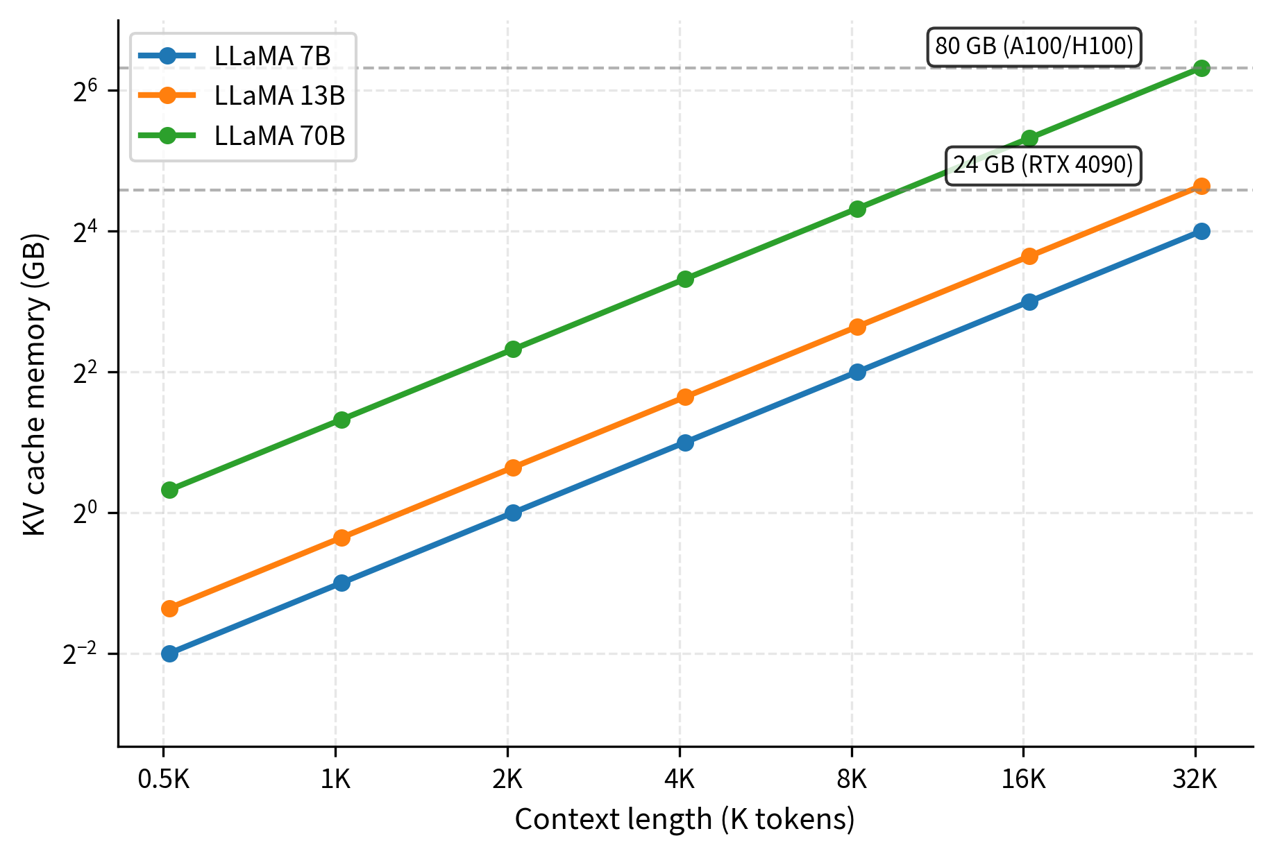
Larger models and longer contexts exacerbate the memory pressure, creating significant challenges for deployment at scale. The following table shows KV cache sizes for various model configurations, illustrating how the requirements grow across different architectural choices:

The cache memory scales linearly with both model size (via the $L \times d_{\text{model}}$ product) and context length. This linear scaling in context length, combined with the quadratic scaling of the attention computation itself, makes long-context inference particularly challenging. A model like GPT-4 with a 128K context window requires hundreds of gigabytes per sequence, necessitating distributed systems and sophisticated memory management strategies.

Efficient cache management involves critical decisions about memory allocation strategies, handling variable sequence lengths across concurrent requests, and managing batched generation effectively. These operational considerations often determine whether a deployment can achieve its throughput and latency targets.

Static allocation pre-allocates cache tensors for the maximum sequence length at the start of generation. This approach reserves all memory upfront, avoiding the overhead of repeated memory allocation during the generation process. Static allocation is preferred when:

• Maximum sequence length is known in advance
• Memory fragmentation must be avoided
• Consistent latency is required

Dynamic allocation grows the cache as needed, typically by allocating larger tensors and copying existing data when the current allocation is exhausted. This saves memory for shorter sequences but introduces allocation overhead and potential fragmentation. Modern frameworks often use a hybrid approach, allocating in chunks (e.g., 128 or 256 tokens at a time) to balance these tradeoffs.

When generating for multiple sequences simultaneously, cache management becomes more complex because different sequences may have different lengths. The typical approaches are:

• Padding: Allocate cache based on the longest sequence in the batch, padding shorter sequences. Simple but wasteful when sequence lengths vary significantly.
• Separate caches: Maintain independent cache tensors per sequence. Avoids wasted memory but complicates the attention computation and prevents batched matrix operations.
• Paged attention: Allocate cache in fixed-size blocks and track which blocks belong to which sequence. This approach, which we'll explore in detail in the upcoming chapter on Paged Attention, enables efficient memory utilization with variable-length sequences.

When a sequence reaches the model's maximum context length, the system must decide how to proceed:

• Truncation: Simply stop accepting new tokens or drop the oldest tokens
• Sliding window: Maintain only the most recent $W$ tokens, discarding older ones (as used in Mistral's architecture, discussed in Part XIX)
• Attention sinks: Keep initial tokens plus recent tokens, leveraging the attention sink phenomenon we covered in Part XV

Each strategy has tradeoffs between memory usage, coherence over long conversations, and computational complexity.

Let's build a simple KV cache implementation to see how these concepts work in practice.

Now let's demonstrate how the cache accelerates generation:

The output confirms that the cache has been initialized with the 8 prompt tokens. The key cache shape shows we have stored the projection results for these tokens, ready to be attended to by future generation steps.

The cache has grown by 5 tokens, now containing the history for 13 tokens total.

Let's compare the computational savings: The crucial detail is that we only processed the 5 new tokens through the model's projection layers, yet the attention mechanism had access to the full 13-token history via the cache.

The savings are substantial. For generation, the projection computation savings grow quadratically with sequence length.

A critical property of KV caching is that it must produce identical outputs to non-cached attention. Let's verify this:

The numerical equivalence confirms that caching is purely an optimization: it changes how we compute the result, not what we compute.

Let's measure actual memory consumption for different configurations:

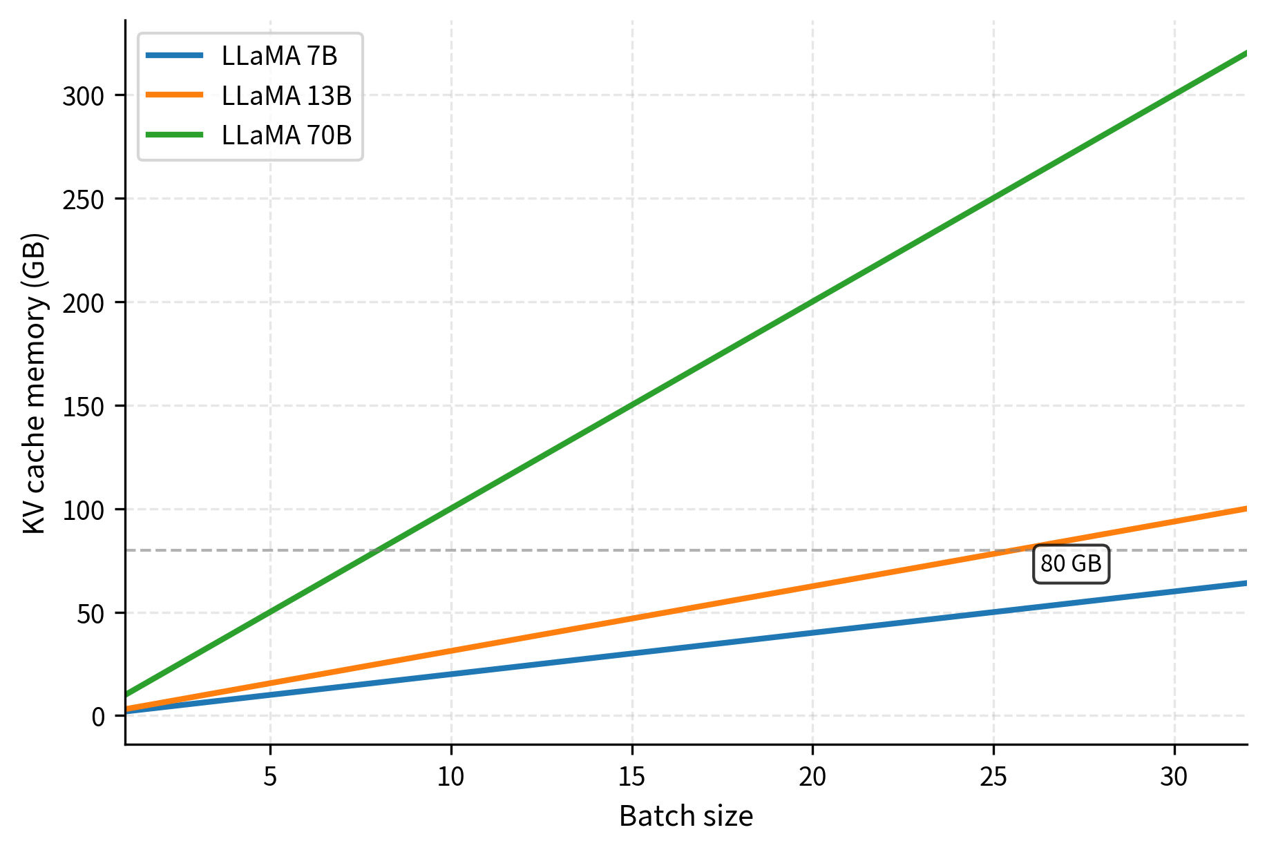
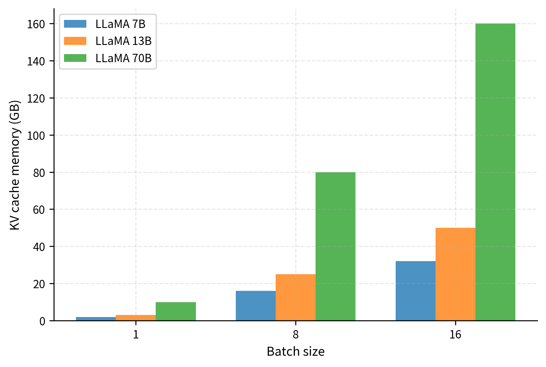
As context length increases, memory usage grows linearly. For the LLaMA-70B model, a single sequence at 8192 context requires 20 GB of cache memory, which is significant even for high-end hardware.

These numbers reveal why KV cache memory management is critical for production systems. A LLaMA-70B model serving 32 concurrent requests at 4K context requires over 160 GB just for the KV cache, exceeding what most single GPUs can provide.

The key parameters for the KV cache implementation are:

• d_model: The dimensionality of the model's hidden states.
• num_heads: The number of attention heads.
• head_dim: The dimension of each attention head ($d_{\text{model}} / \text{num\_heads}$).
• max_seq_len: The maximum sequence length the cache can store.
• batch_size: The number of sequences processed simultaneously.

KV caching introduces several challenges that drive ongoing research in inference optimization.

Memory consumption scales linearly with sequence length. While this is better than the quadratic scaling we'd face without caching, it still creates a hard constraint on context length and batch size. A server with 80 GB of GPU memory might fit the model weights comfortably but struggle to serve multiple long-context requests concurrently. This tension between throughput and context length is fundamental to LLM deployment.

Memory fragmentation becomes problematic with variable-length requests. When different sequences in a batch have different lengths, naive approaches either waste memory through padding or sacrifice batching efficiency. Production systems must carefully manage cache allocation to maximize GPU utilization. The upcoming chapter on Paged Attention addresses this with a memory management approach inspired by operating system virtual memory.

The cache must persist across the entire generation process. Unlike model weights that are read-only during inference, the KV cache is constantly updated. This means the cache cannot be easily offloaded to CPU during generation without incurring significant latency for memory transfers. Systems that need to handle many concurrent requests must carefully orchestrate which caches are active on GPU at any moment.

Grouped-Query Attention reduces cache size. As we discussed in Part XIX, architectures like LLaMA 2 70B use Grouped-Query Attention (GQA), where multiple query heads share a single key-value head. This reduces KV cache size proportionally. For example, if 8 query heads share 1 KV head, the cache is 8× smaller. This architectural choice was motivated specifically by the memory constraints we've described here.

The KV cache is a fundamental optimization that makes autoregressive generation practical. By storing and reusing the key and value projections from attention, we avoid recomputing the same values at every generation step. This reduces the computational overhead from quadratic to linear in the number of generated tokens.

The key concepts covered in this chapter are:

• Redundancy problem: Without caching, each generation step recomputes K and V for all previous tokens, wasting computation
• Cache structure: Separate K and V tensors per layer, growing with sequence length, storing projections for all processed tokens
• Memory requirements: Cache size scales as $2 \times L \times d_{\text{model}} \times T \times \text{bytes}$, easily reaching multiple gigabytes for long sequences
• Prefill vs decode: The initial prompt processing (prefill) populates the cache, while subsequent generation steps (decode) each process only one token
• Cache management: Decisions about static vs dynamic allocation, batching strategies, and context length limits significantly impact deployment efficiency

Understanding KV cache mechanics is essential for working with modern LLMs, as cache memory often becomes the primary constraint on throughput and context length. The next chapter examines KV cache memory in greater detail, followed by Paged Attention's approach to efficient memory management and techniques for compressing the cache to extend context lengths further.

Ready to test your understanding? Take this quick quiz to reinforce what you've learned about KV cache optimization in transformer inference.