

Discover how Activation-aware Weight Quantization protects salient weights to compress LLMs. Learn the algorithm, scaling factors, and AutoAWQ implementation.

This article is part of the free-to-read Language AI Handbook
Choose your expertise level to adjust how many terms are explained. Beginners see more tooltips, experts see fewer to maintain reading flow. Hover over underlined terms for instant definitions.
AWQ
In the previous chapter, we explored GPTQ's approach to quantization, which uses second-order Hessian information to minimize quantization error layer by layer. While GPTQ achieves impressive results, its reliance on expensive matrix inversions and sequential weight updates creates computational overhead that scales with model size. Activation-aware Weight Quantization (AWQ) takes a fundamentally different approach: instead of trying to optimally quantize all weights, it focuses on identifying and protecting the small subset of weights that matter most.
The core insight behind AWQ is straightforward. Not all weights in a neural network contribute equally to output quality. A small fraction of weights, perhaps 0.1-1% depending on the layer, have an outsized impact on model predictions. If we can identify these salient weights and protect them from aggressive quantization, we can apply standard low-bit quantization to everything else with minimal degradation. The key question becomes: how do we identify which weights are salient?
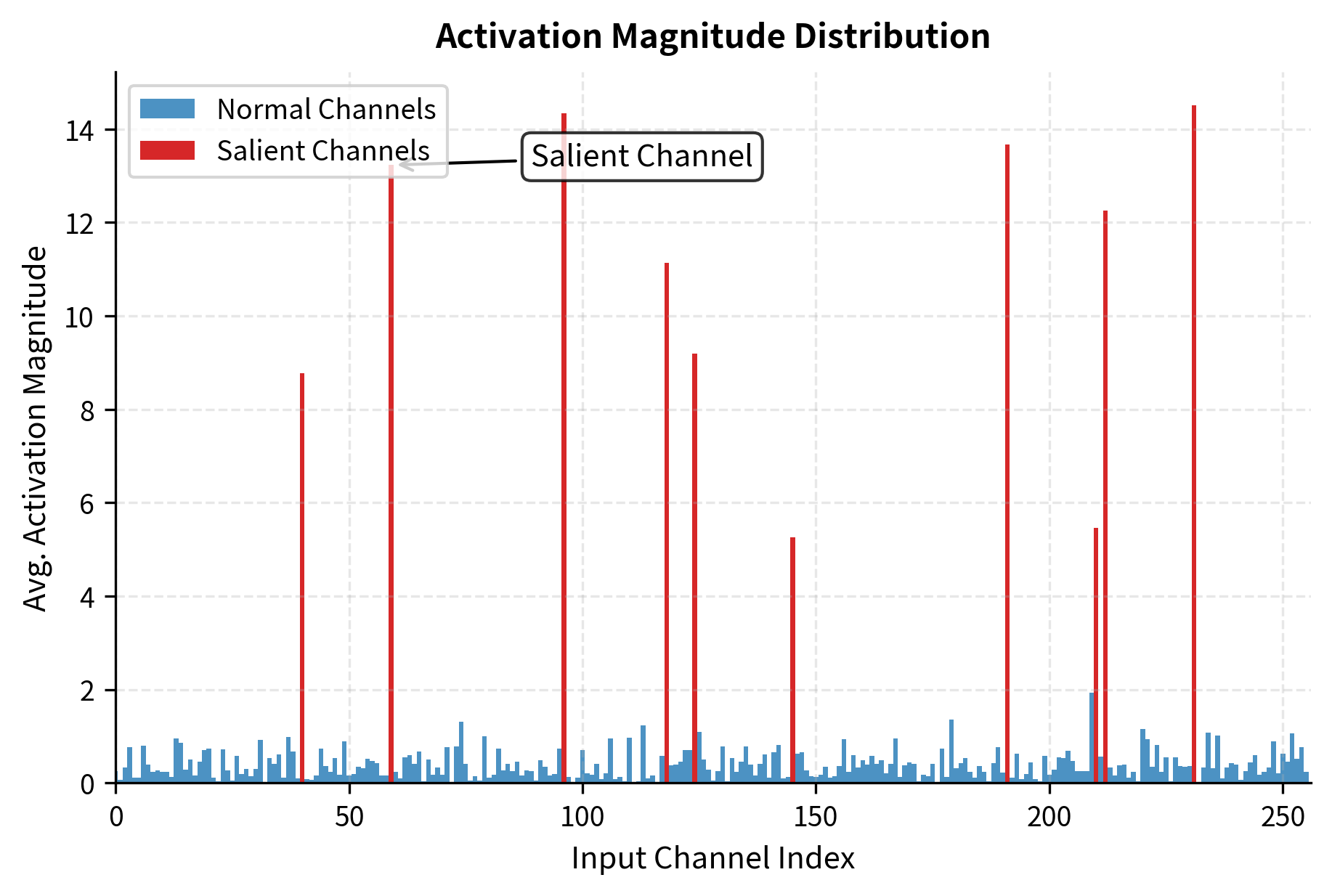
AWQ analyzes the activations. Weights that consistently multiply large activation values have more influence on the output than weights that typically see near-zero activations. By analyzing activation magnitudes across a calibration dataset, AWQ identifies salient weights and applies per-channel scaling factors that effectively give these weights more precision in the quantized representation.
Salient Weight Preservation
The observation underlying AWQ comes from analyzing weight and activation distributions in transformer models. To understand why some weights matter more than others, consider the forward pass through a neural network. Every linear layer performs a weighted sum of its inputs, but not all terms in that sum contribute equally to the final result. Consider a linear layer computing:
where:
- : the output vector containing the results of the linear transformation
- : the weight matrix containing the layer's learnable parameters
- : the input activation vector representing the features from the previous layer
The contribution of weight to output element is . This means a weight's actual impact depends not just on its magnitude but on the magnitude of the activation it multiplies. A weight with value 0.5 that consistently multiplies activations of magnitude 10 contributes far more to the output than a weight with value 2.0 that typically multiplies activations near zero. This observation forms the conceptual foundation of AWQ: the importance of a weight cannot be assessed in isolation but must be understood in the context of the activations it operates upon.
Weights that consistently multiply large activation values across the calibration dataset. These weights have disproportionate influence on model outputs, making their quantization errors more harmful to overall model quality.
Empirical analysis of large language models reveals that activation distributions are highly non-uniform across input channels. Some channels consistently produce large activations across many different inputs, while others typically remain near zero. This non-uniformity is not random; it reflects the learned structure of the model, where certain feature dimensions have become more important during training. This non-uniformity creates an opportunity for more intelligent quantization. If channel always has small activations, quantization errors in the weights connecting to that channel have minimal impact on the final computation. But if channel consistently produces large activations, those weights are salient and require protection because any error in their representation will be amplified by the large activation values.
The simplest approach to protecting salient weights would be to keep them in higher precision, creating a mixed-precision representation where important weights use 8 or 16 bits while less important weights use 4 bits. However, mixed-precision schemes complicate hardware implementation and sacrifice some of the memory and speed benefits we seek from quantization. Inference kernels optimized for uniform 4-bit weights cannot efficiently handle a mix of precisions, and the irregular memory access patterns that result from mixed precision degrade performance. AWQ takes a more clever approach: it uses scaling factors to effectively "hide" more precision in the quantized representation for salient weights while maintaining a uniform bit width throughout the model.
The Scaling Factor Insight
To understand AWQ's approach, recall from our discussion of quantization basics that the quantization error for a weight scales with the quantization step size. The step size determines how far apart adjacent representable values are in the quantized representation. When we quantize to bits with scale , the maximum error is approximately , since any real value can be at most half a step away from the nearest quantization level. For a standard per-tensor or per-channel quantization scheme, the scale is determined by the range of values being quantized:
where:
- : the quantization scale (step size), determining the distance between adjacent representable values
- : the maximum value in the weight tensor, defining the upper bound of the dynamic range
- : the minimum value in the weight tensor, defining the lower bound of the dynamic range
- : the quantization bit width (e.g., 4 for INT4)
- : the maximum integer value representable with bits (the number of discrete levels minus one)
This formula reveals an important insight: the quantization error is determined by how much of the available range each weight occupies. Weights that use more of the quantization range effectively receive finer resolution, while weights that occupy only a small portion of the range are represented more coarsely.
Now consider what happens when we multiply a weight by a constant before quantization, then divide by after dequantization. The weight's contribution to the output is unchanged because the scaling operations cancel out, but its quantization behavior shifts in a favorable way. The scaled weight occupies more of the quantization range, effectively getting finer granularity in the discrete representation. When we dequantize and divide by , the quantization error is also divided by , meaning the effective error in the original weight space is reduced by the same factor.
The catch is that scaling up one weight affects the overall range, potentially increasing quantization error for other weights in the same quantization group. If we scale up salient weights without adjusting anything else, the quantization scale increases to accommodate the larger values, and non-salient weights receive coarser quantization as a result. This is where the activation-awareness becomes crucial. If weight multiplies activations that are on average times larger than typical, scaling that weight up by while scaling down the corresponding activation channel by preserves the computation while reducing quantization error for that salient weight. The inverse scaling on the activation side can be absorbed into preceding layers, making the transformation invisible at inference time.
Mathematically, for an input channel , we can apply a scaling factor to the weights and absorb the inverse scaling into the preceding layer or activation:
where:
- : the output value for neuron
- : the weight connecting input to output
- : the input activation at channel
- : the scaling factor applied to channel
The key insight is that we want to be larger for channels with larger typical activations, protecting those salient weights with more precision in the quantized representation. Channels with large activations will have their weights scaled up, giving those weights more quantization levels to work with. Channels with small activations will have their weights left mostly unchanged or even scaled down slightly. The net effect is a redistribution of quantization precision from where it is wasted (low-activation channels) to where it matters most (high-activation channels).
The AWQ Algorithm
AWQ determines optimal per-channel scaling factors by analyzing activation statistics from a small calibration dataset. Unlike GPTQ, which requires solving optimization problems involving Hessian matrices, AWQ relies on straightforward statistical measurements that can be computed efficiently in a single forward pass. The algorithm proceeds through several stages: activation collection, scale computation, weight transformation, and standard quantization.
Activation Statistics Collection
The first step is running a calibration set through the model and collecting activation statistics. This calibration set need not be large; typically a few hundred examples suffice to obtain stable estimates of activation magnitudes. For each linear layer, we record the average magnitude of each input channel across the calibration examples:
where:
- : the average activation magnitude for channel , serving as a proxy for the channel's importance
- : the total number of calibration samples used to estimate statistics
- : the activation value at channel for the -th sample
- : the absolute magnitude of the activation, capturing signal strength regardless of sign
Taking the absolute value ensures we capture the activation strength regardless of whether the values tend to be positive or negative. The average across samples smooths out noise from individual examples and reveals the underlying pattern of which channels consistently carry strong signals. These channel-wise activation magnitudes tell us which weights are salient: weights in columns corresponding to high values are more important because they multiply large numbers during typical inference.
Computing Optimal Scaling Factors
Given activation statistics, AWQ computes scaling factors that balance two competing objectives:
- Protect salient weights: Channels with large activations should get larger scaling factors, expanding their weights to occupy more of the quantization range
- Don't harm other weights: Extreme scaling factors can hurt non-salient weights by compressing their share of the quantization range too aggressively
Finding the right balance requires a formula that grows with activation magnitude but not too aggressively. AWQ uses a simple but effective formula for the scaling factors:
where:
- : the calculated scaling factor for channel , determining how much to magnify the weights in this channel
- : the average activation magnitude for channel
- : the maximum average activation magnitude across all channels, serving as the normalization reference
- : a hyperparameter controlling scaling strength, balancing the protection of salient weights against the distortion of others
The normalization by ensures that scaling factors lie in the range , with the channel having the largest activations receiving a scaling factor of exactly 1. This prevents any channel from being scaled up, which would expand the overall weight range. Instead, less important channels are effectively scaled down relative to the most important ones.
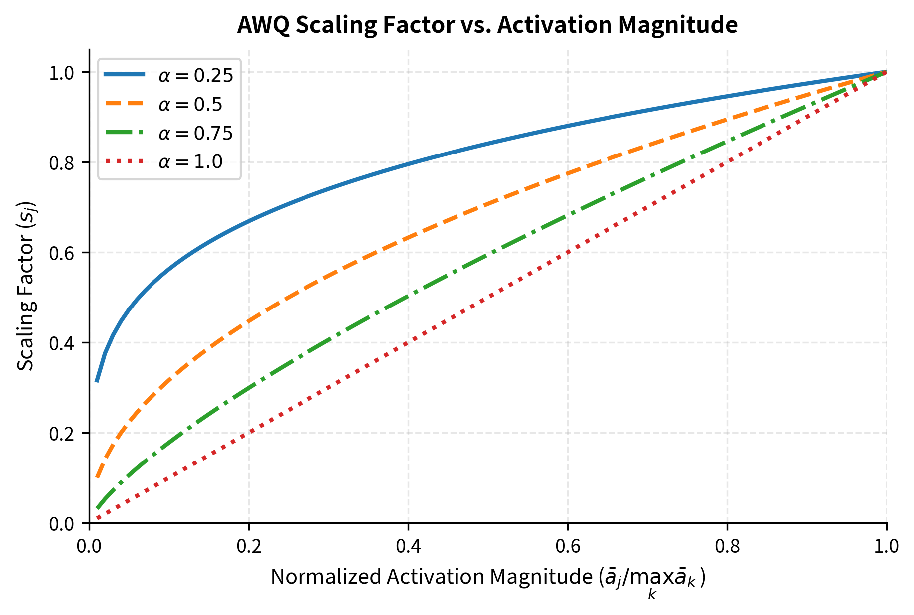
When , all scaling factors are 1 (no adjustment), and AWQ reduces to standard quantization without any activation-aware optimization. When , scaling factors are directly proportional to relative activation magnitudes, providing maximum differentiation between channels. In practice, values between 0.25 and 0.75 work well, with the original AWQ paper using grid search to find optimal values per layer.
The exponent provides a smooth tradeoff between the two objectives. Small values provide modest protection to salient weights while minimizing disruption to other weights, resulting in a more uniform treatment across channels. Larger values provide stronger protection for the most salient weights but may harm non-salient weights by compressing their range more aggressively. The optimal choice depends on the specific weight and activation distributions in each layer.
Weight Transformation and Quantization
With scaling factors computed, AWQ transforms the weights before applying standard quantization. The transformation is straightforward: for each input channel , the corresponding column of weights is multiplied by the scaling factor :
where:
- : the transformed (scaled) weight, which will be input to the quantization process
- : the original weight parameter
- : the scaling factor for channel , expanding the weight's magnitude to utilize more of the quantization range
This multiplication stretches the weights for high-activation channels while compressing those for low-activation channels. The resulting weight distribution is better suited for quantization because the most important weights now span a larger portion of the quantization range.
The inverse scaling must be applied somewhere to preserve the original computation. AWQ handles this by fusing the inverse scaling into the preceding layer's weights or biases. For transformer models, the LayerNorm or RMSNorm parameters can absorb this scaling efficiently. Since normalization layers output to the same channels that serve as inputs to the linear layer, multiplying the normalization scale by for each channel achieves the needed compensation without adding any runtime overhead.
After transformation, AWQ applies standard group-wise INT4 quantization to the scaled weights:
where:
- : the quantized-then-dequantized weight approximation, representing the value actually used during inference
- : the scaled weight being quantized
- : the quantization scale for the weight group, mapping the integer grid back to real values
- : the rounding operation to the nearest integer, which introduces the quantization error
The rounding operation is where information is lost, as continuous values are mapped to the nearest point on a discrete grid. However, because salient weights have been scaled up, they now occupy more grid points and suffer proportionally less error.
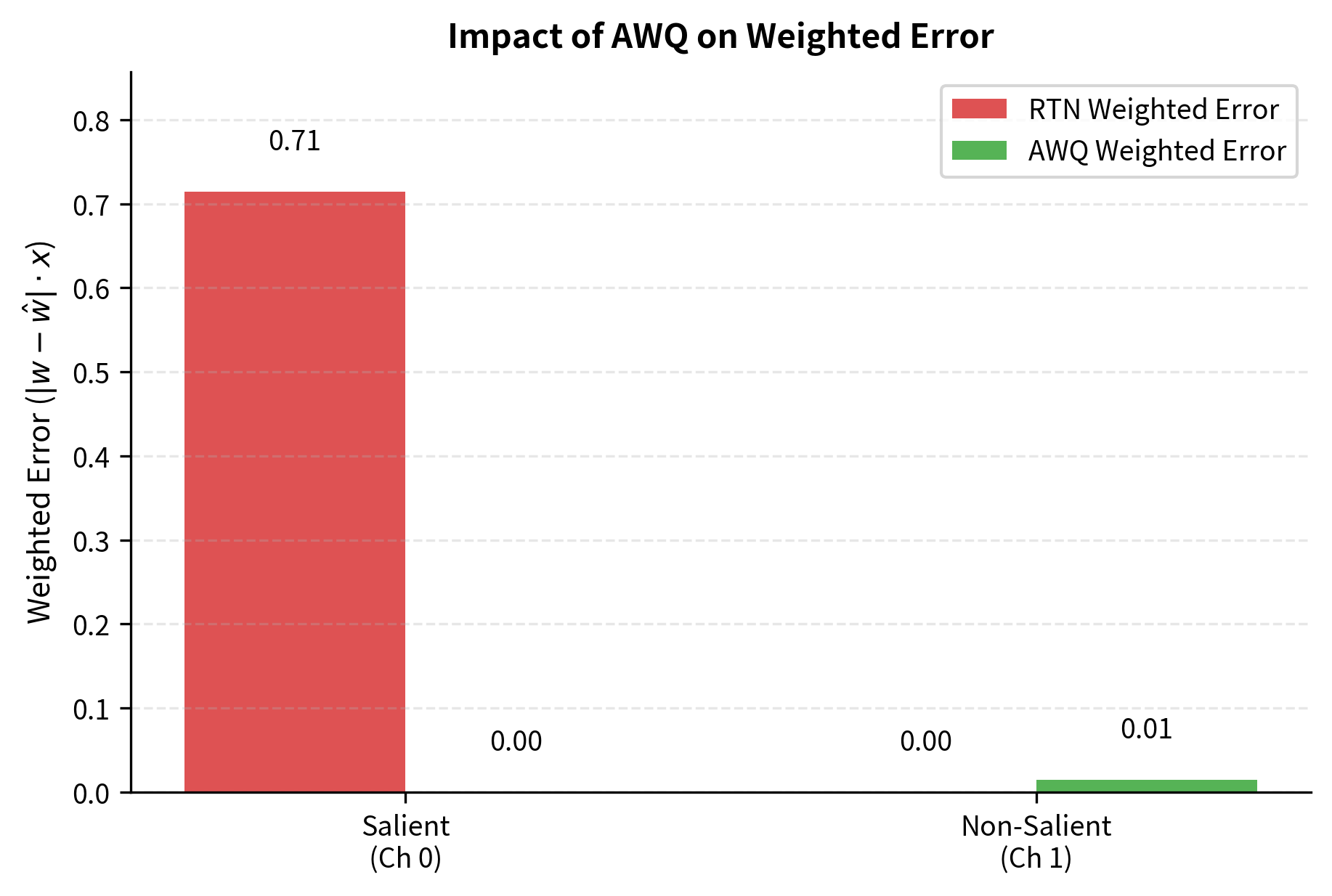
The final dequantized value, after applying the inverse channel scaling, has reduced error for salient weights:
where:
- : the effective quantization error for weight in the original unscaled domain
- : the base quantization error (approximately ) inherent to the INT4 grid
- : the channel scaling factor; dividing by this reduces the effective error magnitude for salient (scaled-up) channels
For salient channels where , the effective error is reduced proportionally. This is the core mechanism by which AWQ achieves better accuracy than naive quantization: it redistributes precision to where it matters most, reducing errors in the computations that have the largest impact on model outputs.
Grid Search Optimization
While the formula-based scaling provides a good starting point, AWQ refines the scaling factors through grid search. The exponent controls the aggressiveness of the scaling, and the optimal value varies across layers depending on their specific weight and activation distributions. For each layer, the algorithm:
- Generates candidate values (typically 0, 0.25, 0.5, 0.75, 1.0)
- For each , computes scaling factors and quantized weights
- Evaluates quantization error using mean squared error on calibration outputs
- Selects the that minimizes error
This per-layer grid search adds minimal computational overhead since we're only searching over a handful of values, unlike GPTQ's expensive Hessian computations. The search space is tiny, requiring only a few forward passes through each layer to evaluate the candidates. The resulting layer-specific values allow AWQ to adapt to the heterogeneous structure of modern neural networks, where different layers may have very different activation and weight distributions.
Implementation
Let's walk through a practical AWQ quantization using the AutoAWQ library, which implements the full AWQ algorithm with optimized kernels for inference.
We'll demonstrate AWQ quantization on a small model to show the workflow. The process involves loading the model, configuring quantization parameters, and running the algorithm on a calibration dataset.
AWQ requires a calibration dataset to compute activation statistics. The calibration set should be representative of the model's intended use case. For general-purpose language models, a diverse set of text samples works well.
The AWQ quantization configuration specifies the bit width, group size, and other parameters. Group size controls how many weights share a quantization scale, with smaller groups providing better accuracy at the cost of more scale storage.
The quantize method runs the full AWQ algorithm: it collects activation statistics from the calibration data, computes optimal per-channel scaling factors using grid search, transforms and quantizes the weights, and fuses the inverse scaling into preceding layers.
The output confirms the successful creation of the quantized model directory, which now contains the compressed weights and configuration files needed for inference.
Loading and Using AWQ Models
Once quantized, AWQ models can be loaded efficiently for inference. The AutoAWQ library provides optimized CUDA kernels that perform dequantization on-the-fly during matrix multiplication.
The generated text demonstrates that the 4-bit quantized model retains the linguistic capabilities of the original, producing coherent and contextually appropriate output.
The fuse_layers=True option enables additional optimizations that combine sequential operations, reducing memory bandwidth requirements and improving throughput.
Understanding the Quantization Structure
AWQ stores quantized weights in a packed format where multiple 4-bit values share bytes. Let's examine the structure of a quantized layer:
The inspection reveals the internal structure of AWQ quantization: weights are packed into INT32 tensors (qweight) while scales are kept in higher precision (scales). The compression ratio confirms the expected 4x reduction in memory usage compared to FP16.
Key Parameters
The key parameters for AWQ quantization are:
- w_bit: The bit width for weight quantization (e.g., 4).
- q_group_size: The number of weights that share a single scaling factor. Smaller groups improve accuracy but increase memory usage.
- zero_point: Whether to use asymmetric quantization (True) or symmetric (False).
- version: The quantization kernel version to use (e.g., "GEMM" for general matrix multiplication optimized kernels).
AWQ vs GPTQ
Both AWQ and GPTQ achieve INT4 quantization with minimal accuracy loss, but they approach the problem from fundamentally different angles. Understanding these differences helps you choose the right method for your use case.
Algorithmic Philosophy
GPTQ, as we discussed in the previous chapter, treats quantization as an optimization problem. It uses second-order information from the Hessian to determine how to round each weight to minimize the overall squared error. This approach is mathematically principled and provides optimal solutions within its framework, but computing and inverting the Hessian adds significant computational overhead.
AWQ takes an empirical, observation-driven approach. It recognizes that a small subset of weights dominates output quality and focuses protection on those weights. Rather than optimizing the quantization of each individual weight, AWQ optimizes the distribution of precision across weight groups by choosing appropriate scaling factors.
Quantization Speed
GPTQ's layer-by-layer optimization with Hessian computation creates substantial overhead, particularly for larger models. Quantizing a 7B parameter model with GPTQ typically takes 30-60 minutes on a modern GPU. AWQ's simpler algorithm, based on activation statistics and grid search over a handful of scaling parameters, completes much faster, often 2-4x quicker than GPTQ for the same model.
The speed difference becomes more pronounced as model size increases. For 70B+ parameter models, AWQ's advantage is particularly significant, with quantization completing in hours rather than many hours or days.
Accuracy Comparison
Both methods achieve excellent accuracy retention, typically within 0.5-1 perplexity points of the original FP16 model when quantizing to INT4. Empirical comparisons show they perform similarly across a range of benchmarks:
| Model Size | Method | Wiki2 PPL (FP16) | Wiki2 PPL (INT4) | Delta |
|---|---|---|---|---|
| 7B | GPTQ | 5.68 | 5.85 | +0.17 |
| 7B | AWQ | 5.68 | 5.82 | +0.14 |
| 13B | GPTQ | 5.09 | 5.20 | +0.11 |
| 13B | AWQ | 5.09 | 5.18 | +0.09 |
| 70B | GPTQ | 3.32 | 3.41 | +0.09 |
| 70B | AWQ | 3.32 | 3.40 | +0.08 |
AWQ often edges out GPTQ slightly on perplexity benchmarks, though differences are within noise margins. The more significant accuracy advantage of AWQ emerges in out-of-distribution scenarios: AWQ's activation-based importance estimation generalizes better to inputs outside the calibration distribution.
Inference Kernel Support
GPTQ has been available longer and has broader kernel support across different hardware platforms. Libraries like llama.cpp, ExLlama, and text-generation-inference all support GPTQ formats.
AWQ kernels are newer but have been rapidly adopted. The AutoAWQ library provides optimized CUDA kernels, and major inference frameworks like vLLM and TensorRT-LLM now include AWQ support. AWQ's simpler weight transformation (per-channel scaling rather than arbitrary linear combinations) also makes kernel implementation more straightforward.
When to Choose Each Method
Choose GPTQ when:
- You need maximum compatibility with existing inference infrastructure
- You're willing to spend more time on quantization for potentially optimal results
- You're quantizing smaller models where quantization time is not a bottleneck
Choose AWQ when:
- You're quantizing very large models (65B+) and quantization speed matters
- You need robust accuracy across diverse input distributions
- You're deploying on platforms with AWQ kernel support (vLLM, TensorRT-LLM)
Benefits and Practical Considerations
AWQ provides several advantages that make it particularly attractive for deploying large language models in resource-constrained environments.
Memory Efficiency
Like other INT4 quantization methods, AWQ reduces model memory footprint by approximately 4x compared to FP16. A 7B parameter model drops from ~14GB to ~4GB, enabling deployment on consumer GPUs. A 70B model fits in ~40GB, making it accessible on high-end professional GPUs rather than requiring multi-GPU setups.
The memory savings extend beyond weight storage. AWQ's simpler transformation (per-channel scaling) adds minimal metadata overhead compared to methods that store additional calibration information. The scales and zero points required for group-wise quantization typically add only 0.5-1% to the compressed model size.
Inference Speed
AWQ achieves throughput improvements of 1.5-3x over FP16 inference on modern GPUs, depending on the specific hardware and model architecture. These speedups come from two sources:
- Reduced memory bandwidth: Reading 4-bit weights requires 4x less bandwidth than 16-bit weights, and modern inference is often memory-bandwidth limited
- Efficient dequantization: AWQ's per-channel scaling maps cleanly to tensor operations, enabling highly optimized dequantization kernels
The actual speedup depends heavily on your inference setup. Memory-bound scenarios (large batch sizes, long sequences, limited GPU memory bandwidth) see the largest improvements. Compute-bound scenarios see smaller but still significant gains.
Calibration Sensitivity
AWQ requires only a small calibration dataset, typically 128-512 samples, to compute reliable activation statistics. The algorithm is robust to the specific calibration samples chosen, as it only uses them to compute channel-wise average magnitudes. This contrasts with methods that use calibration data for layer-wise optimization, which can overfit to the specific samples.
However, the calibration data should still be representative of the model's intended use case. Quantizing a code generation model using only English prose samples may not yield optimal results for code completion tasks, since activation patterns differ between domains.
Limitations and Edge Cases
AWQ's activation-awareness can struggle in certain scenarios. If a weight is truly important but happens to see small activations on the calibration set, AWQ will not protect it. This can occur when:
- The calibration set misses important input patterns
- Certain model behaviors only activate rarely but crucially
- Domain shift between calibration and deployment data is significant
Additionally, AWQ's assumption that per-channel scaling is sufficient may not capture all forms of weight saliency. Some weights may be important due to their interaction with other weights in complex ways that per-channel statistics don't capture. GPTQ's Hessian-based approach can sometimes identify these subtler patterns.
For most practical deployments, these limitations are minor. AWQ consistently achieves excellent results across diverse models and tasks, and its speed and simplicity advantages make it a compelling default choice for INT4 quantization.
Summary
AWQ represents a shift in quantization philosophy, from optimizing all weights equally to protecting the small subset that matters most. The key ideas covered in this chapter include:
Salient weight identification: AWQ observes that weights multiplying large activations have disproportionate impact on outputs. By analyzing activation magnitudes from a calibration dataset, it identifies which weights deserve protection.
Per-channel scaling: Rather than keeping salient weights at higher precision, AWQ uses scaling factors to effectively give them more resolution in the quantized representation. Weights are scaled up before quantization, with the inverse scaling fused into preceding layers.
Efficient algorithm: AWQ avoids GPTQ's expensive Hessian computations in favor of simple activation statistics and grid search over scaling hyperparameters, enabling faster quantization of large models.
Practical tradeoffs: AWQ and GPTQ achieve similar accuracy, but AWQ offers faster quantization and often better generalization to out-of-distribution inputs. GPTQ has broader ecosystem support due to its earlier release.
The next chapter explores the GGUF format, which provides a standardized way to store and distribute quantized models across different inference engines and hardware platforms.
Quiz
Ready to test your understanding? Take this quick quiz to reinforce what you've learned about Activation-aware Weight Quantization (AWQ).

Comments