

Discover how GPTQ optimizes weight quantization using Hessian-based error compensation to compress LLMs to 4 bits while maintaining near-FP16 accuracy.

This article is part of the free-to-read Language AI Handbook
Choose your expertise level to adjust how many terms are explained. Beginners see more tooltips, experts see fewer to maintain reading flow. Hover over underlined terms for instant definitions.
GPTQ
In the previous chapters on INT8 and INT4 quantization, we explored straightforward approaches to weight compression: round each weight to the nearest representable value in the target format. While these methods work reasonably well, they treat each weight independently, ignoring the complex interactions between weights in a neural network. A small rounding error in one weight might be catastrophic for model quality, while a larger error in another weight might barely matter.
GPTQ (GPT Quantization) takes a fundamentally different approach. Rather than treating quantization as a simple rounding problem, GPTQ frames it as an optimization problem: given a layer's weights, find the quantized values that minimize the layer's output error. The key insight is that when you quantize one weight, you can partially compensate for the resulting error by adjusting the remaining weights before they too are quantized.
This compensation mechanism, combined with algorithmic optimizations, allows GPTQ to achieve low quantization error. Models quantized with GPTQ to 4 bits often perform nearly as well as their full-precision counterparts, enabling LLMs with tens of billions of parameters to run on consumer GPUs. GPTQ was one of the first methods to make models like LLaMA-65B practically usable on hardware that would otherwise be unable to load them.
The Layer-Wise Reconstruction Objective
To understand how GPTQ approaches quantization, we must first establish what it means to quantize well. The fundamental question is: what objective should we optimize? One natural answer might be to minimize the difference between original and quantized weights directly. However, this ignores a crucial insight: not all weight errors are equally harmful. What truly matters is how quantization affects the layer's output, because the output is what downstream computations depend upon.
GPTQ operates on one layer at a time, treating each layer's quantization as an independent optimization problem. This layer-wise decomposition is both a practical necessity and a reasonable approximation. Consider a linear layer with weights and inputs , where represents the number of calibration tokens we use to estimate the layer's behavior. The goal is to find quantized weights that minimize the reconstruction error:
where:
- : the reconstruction error (loss) for the quantized weights
- : the original high-precision weight matrix
- : the quantized weight matrix
- : the input matrix (calibration data)
- : the Frobenius norm (square root of the sum of squared elements)
This loss function measures how much the layer's output changes due to quantization. Notice that we are comparing outputs, not weights directly. This distinction is essential: a weight that interacts with large input values will have a greater impact on the output than a weight that sees only small inputs. The Frobenius norm provides a natural way to aggregate these output differences into a single scalar that we can minimize.
Why focus on layer outputs rather than the final model loss? Computing gradients through the entire model for every quantization decision would be prohibitively expensive. Each quantization decision would require a full forward and backward pass, and with millions of weights to quantize, this approach simply does not scale. The layer-wise approach makes GPTQ tractable: we only need to run a forward pass through the model once to collect each layer's inputs, then we can quantize each layer independently. This factorization reduces a global optimization problem into many smaller, manageable subproblems.
The reconstruction error can be rewritten in a form that reveals important mathematical structure. This reformulation exposes the role of input correlations in determining which weights matter most. Expanding the Frobenius norm using the identity :
where:
- : the trace operator (sum of diagonal elements)
- : the weight error matrix
- : the transpose of the input matrix
The trace operation sums the diagonal elements of the resulting matrix. What emerges from this manipulation is that the loss depends on the weight errors not in isolation, but as weighted by the matrix . This matrix captures how the inputs correlate with each other: if two input dimensions tend to activate together, errors in their corresponding weights will interact.
Define , which we call the Hessian matrix (we'll explain why this name is appropriate shortly). The loss becomes:
where:
- : the trace operator
- : the weight error matrix
- : the Hessian matrix () that captures input correlations
- : a scaling factor arising from the definition of
This quadratic form indicates that the loss is a weighted sum of squared errors, where the weighting comes from the Hessian matrix. Errors in weights that correspond to highly active or correlated inputs are penalized more heavily than errors in weights that rarely contribute to the output.
Since the rows of don't interact in this expression (each output dimension is computed independently as a dot product with the inputs), we can optimize each row separately. This further simplifies our problem: instead of optimizing over all weights simultaneously, we can solve independent problems, each involving only weights. For a single row :
where:
- : a single row of the original weight matrix
- : the corresponding row of quantized weights
- : the Hessian matrix (shared across all rows)
- : the error vector for this row
This weighted squared error gives us the foundation for GPTQ's optimization strategy. The quadratic structure of this loss function is crucial because it enables closed-form solutions for optimal weight updates, as we will see in the following sections.
The Hessian and Its Role
The matrix is called the Hessian because it equals the second derivative of the reconstruction loss with respect to the weights. This naming reflects a connection to optimization theory. The Hessian matrix characterizes the local curvature of the loss landscape, telling us how rapidly the loss changes as we move in different directions through weight space.
To see why this matrix represents second derivatives, consider the loss for a single output neuron. We want to find weights that make the neuron's output match what it would produce with the original weights:
where:
- : the weight vector being optimized
- : the -th input vector from the calibration set
- : the target output scalar (computed using the original weights )
- : the total number of calibration tokens
This is a standard least-squares objective. To find its minimum, we compute the gradient by differentiating with respect to each weight component. The gradient is:
where:
- : the gradient vector of the loss with respect to the weights
- : the weight vector
- : the -th input vector
- : the target output scalar
Taking the derivative once more, we obtain the Hessian, which tells us how the gradient itself changes as we modify the weights. And the Hessian (second derivative) is:
where:
- : the Hessian matrix
- : the second derivative of the loss function
- : the -th input vector
- : the matrix of all calibration inputs
The Hessian captures the curvature of the loss landscape around the current weights. Each element of this matrix has a specific interpretation that guides the quantization process. The diagonal elements indicate how sensitive the loss is to changes in weight . A large value means that small perturbations to this weight cause large changes in the output, making this weight "important" in the sense that we must quantize it carefully. The off-diagonal elements capture interactions between weights: they tell us how changes in one weight affect the optimal value of another. When two weights have a large off-diagonal element, their quantization errors are not independent; an error in one can be partially offset by adjusting the other.
The Hessian is simply a scaled covariance matrix of the layer's inputs. We don't need access to labels or backpropagation; we just need to observe what inputs flow through the layer during a forward pass on calibration data.
This observation has significant practical implications. Computing the Hessian requires only a forward pass through the network on calibration data. We never need to differentiate through the model or compute any target labels. The Hessian emerges naturally from the statistics of the inputs that the layer observes during normal operation. This makes GPTQ a true post-training quantization method: we take a pre-trained model, run it on some representative data, and use the resulting statistics to guide quantization.
Optimal Brain Quantization
GPTQ builds on a framework called Optimal Brain Quantization (OBQ), which itself descends from classical work on neural network pruning. The historical connection is illuminating: pruning and quantization are closely related problems. In pruning, we set certain weights exactly to zero. In quantization, we round weights to the nearest value in a discrete set. Both operations introduce error, and in both cases we want to minimize the impact on the network's output.
The core insight of OBQ is that when you quantize one weight, you can compute the optimal adjustment to all remaining weights that minimizes the resulting increase in loss. This is not a heuristic or approximation; given the quadratic structure of our loss function, there exists a closed-form formula for the best possible compensation.
Suppose we've decided to quantize weight to value . We want to adjust the remaining weights (where denotes the set of weights not yet quantized) to minimize:
where:
- : the original weight vector
- : the quantized weight vector (incorporating both the quantized weight and the adjustment )
- : the Hessian matrix
- : the optimal adjustment vector we want to find for the remaining weights
- : the quantized value for weight
The optimization proceeds as follows. We have committed to a particular quantized value for weight , which introduces an error . The question is: how should we modify the remaining weights to absorb as much of this error as possible? Because our loss is quadratic, we can differentiate with respect to , set the result to zero, and solve for the optimal adjustment.
Taking the derivative and setting it to zero yields the optimal update:
where:
- : the optimal adjustment vector for the remaining unquantized weights
- : the quantization error for the current weight
- : the diagonal element of the inverse Hessian corresponding to weight
- : the elements of the -th column of the inverse Hessian corresponding to the remaining weights
Let's unpack this formula to build intuition for what it means. The numerator is the quantization error for weight , simply the difference between what we wanted and what we got. The denominator represents the inverse curvature, which measures how flexible the loss landscape is with respect to weight ; a larger value implies the model is less sensitive to errors in this weight, which means errors can be more easily absorbed by other weights. When this value is large, the penalty for error in weight is small, making compensation easier. The vector determines how this error should be distributed across remaining weights based on their correlations with weight . Weights that are strongly correlated with (in terms of their effect on the output) receive larger adjustments.
The resulting increase in loss from quantizing weight (after optimal compensation) is:
where:
- : the increase in reconstruction error caused by quantizing weight
- : the squared quantization error
- : the diagonal element of the inverse Hessian (representing the "stiffness" of weight )
This formula tells us exactly how much each quantization decision costs, accounting for optimal compensation. The cost depends on two factors: the squared quantization error and the inverse curvature. Weights where is large can be quantized with relatively low cost even if the rounding error is substantial. Conversely, weights with small values are stiff: even small errors cause significant loss increases.
The GPTQ Algorithm
The naive OBQ approach would quantize weights one at a time, choosing at each step the weight whose quantization causes the smallest loss increase. While this strategy appears straightforward, its computational cost is prohibitive. Each step requires examining all remaining weights to find the best candidate, and after quantizing each weight, we must update the inverse Hessian. This requires operations per weight, yielding complexity per row and for the entire layer. That's far too slow for large models where can be in the thousands.
GPTQ makes three key modifications that reduce the total complexity to while maintaining nearly identical accuracy. The insight is that the optimal quantization order matters less than one might expect. What matters more is performing the compensation correctly.
Column-wise processing: Instead of quantizing weights one at a time in optimal order, GPTQ processes all weights in a fixed column order. Alternatively, it uses a smart ordering based on Hessian diagonals, called ActOrder. Processing columns together enables vectorization, allowing us to quantize all rows of the weight matrix simultaneously for a given column.
Lazy batch updates: Rather than updating all remaining weights after each quantization, GPTQ accumulates updates in blocks and applies them periodically. This improves cache efficiency dramatically because memory access patterns become more predictable and localized.
Cholesky-based inverse updates: Computing and updating the full inverse Hessian is expensive. GPTQ uses the Cholesky decomposition of the inverse Hessian, which can be updated efficiently as columns are processed. The triangular structure of the Cholesky factor allows updates in time per column after an initial factorization.
Here's the algorithm in detail:
-
Collect calibration data: Run a small set of examples through the model, recording each layer's inputs .
-
Compute the Hessian: For each layer, compute and its inverse (or Cholesky factor).
-
Process each row of the weight matrix: For each row :
a. For each column from 0 to :
- Quantize:
- Compute error:
- Update remaining weights:
b. Store the quantized row
-
Replace the layer's weights with their quantized values plus any required metadata (scales, zero points).
The order in which columns are processed affects accuracy. The default left-to-right order works reasonably well, but ActOrder (processing columns in decreasing order of Hessian diagonal) often improves results by quantizing the most important weights first, when there are still many remaining weights to absorb compensation.
Mathematical Details of the Update
The inverse Hessian update is a critical mathematical component that enables efficient processing. After quantizing column , we need to update the inverse Hessian to reflect that column is no longer a free variable. The weight at column has been fixed to its quantized value; it can no longer be adjusted to compensate for future quantization errors.
Let be the inverse Hessian restricted to the remaining (unquantized) weights. After removing column/row , the new inverse is:
where:
- : the updated inverse Hessian element at row , column
- : the current inverse Hessian element at row , column
- : elements from the -th column/row of the current inverse Hessian
- : the diagonal element corresponding to weight
- : indices of the remaining unquantized weights
This formula is a rank-one update that removes the row and column corresponding to . The intuition is that by fixing weight , we eliminate one degree of freedom from our optimization problem. The relationships between remaining weights must be adjusted to account for this lost flexibility. Computing this update naively would cost per column, but the Cholesky decomposition enables a much more efficient approach.
The Cholesky factorization gives us where is lower triangular. This factorization is particularly valuable because the triangular structure directly encodes the sequential dependencies between weights. The -th column of directly gives us the coefficients needed for the weight update, and removing column corresponds to simply moving to the next column of . This reduces the per-column update cost to after the initial factorization.
Calibration Data
GPTQ requires calibration data to estimate the Hessian. The quality and quantity of this data affects quantization results:
-
Quantity: GPTQ typically uses 128-1024 samples. More samples give a better Hessian estimate but increase computation.
-
Representativeness: The calibration data should resemble the data the model will see at inference. Using random text to calibrate a code model yields worse results than using code samples.
-
Sequence length: Longer sequences provide more tokens per sample. Most implementations use 2048 tokens per sequence.
The calibration data doesn't need labels; GPTQ only performs forward passes to collect layer activations. Common choices include random samples from C4 (web text), WikiText (Wikipedia), or domain-specific data for specialized models.
Group Quantization
Standard per-tensor or per-channel quantization uses a single scale and zero point for many weights. GPTQ often employs group quantization, where weights are divided into groups (commonly 128 weights each) that share quantization parameters.
Group quantization provides a middle ground between accuracy and overhead:
-
Per-tensor quantization: One scale for all weights. Minimum storage overhead but potentially high quantization error if weight distributions vary.
-
Per-group quantization: Separate scales for groups of 128 weights. Small overhead (one FP16 scale per 128 INT4 weights = 0.125 bits/weight) with substantially better accuracy.
-
Per-weight quantization: Individual scales per weight. Maximum accuracy but impractical overhead.
With group size 128 and 4-bit weights, the effective storage is approximately 4.125 bits per weight, a tiny overhead for significant accuracy gains.
Implementation with AutoGPTQ
Let's see GPTQ in practice using the AutoGPTQ library, which provides an efficient implementation of the algorithm.
First, we'll load a small model to demonstrate the quantization process:
Let's examine the original model's memory footprint:
The output shows that 4-bit quantization reduces the memory footprint to a quarter of its FP16 size. For this 125M parameter model, this means dropping from over 200 MB to a much more manageable size, illustrating the efficiency gains crucial for deploying larger models.
Now let's implement a simplified version of the GPTQ core algorithm to understand how it works:
Here's the core GPTQ algorithm for a single row of weights:
Let's demonstrate this on a sample weight matrix:
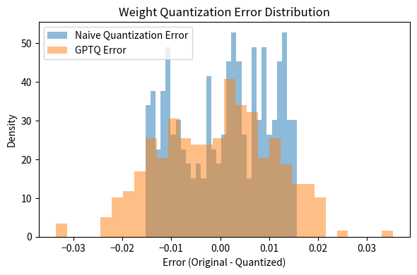
The GPTQ algorithm achieves substantially lower reconstruction error by compensating for each quantization decision. This error compensation is what distinguishes GPTQ from naive round-to-nearest approaches.
Measuring Output Reconstruction Error
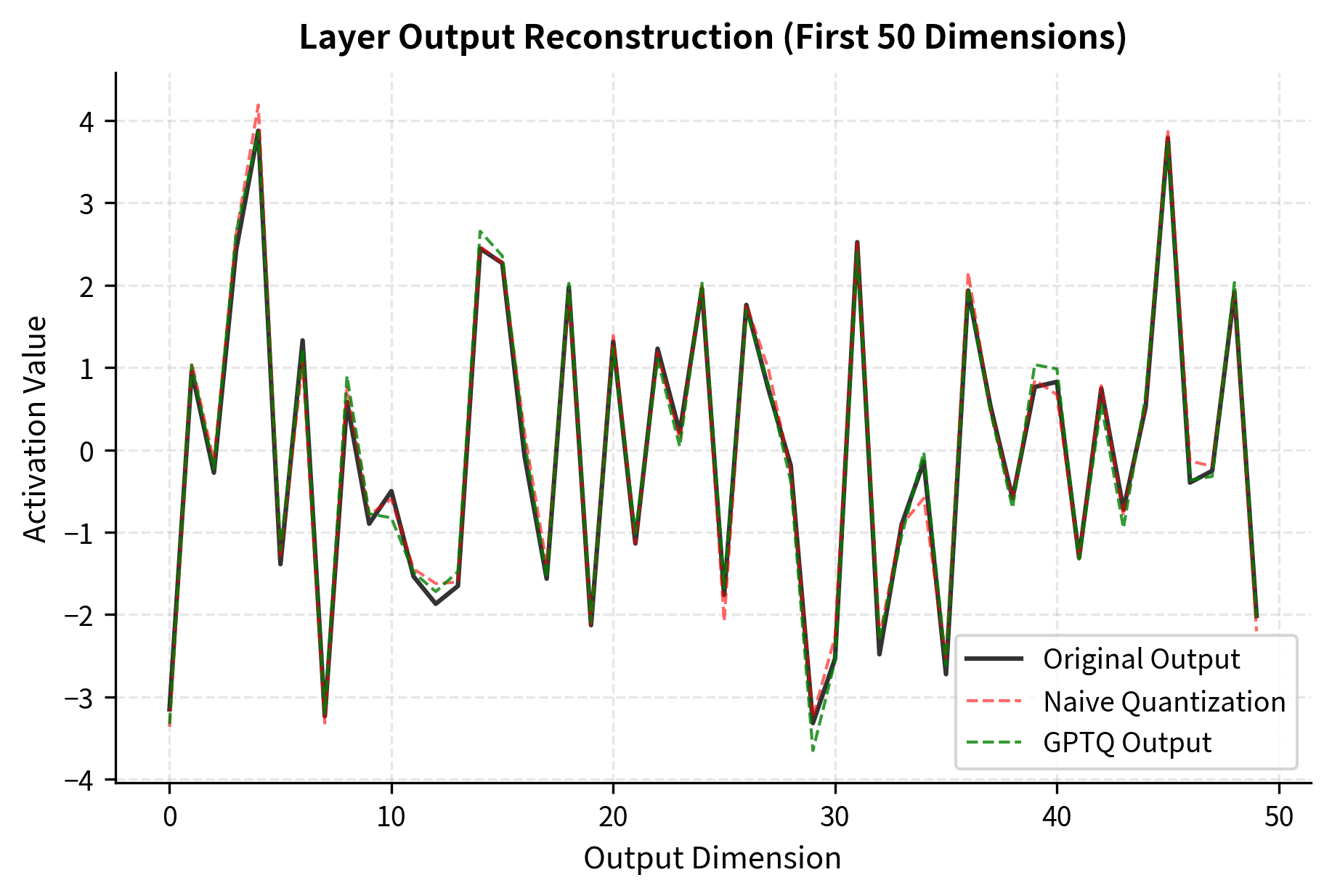
The true measure of quantization quality is the layer output error, not just the weight error. Let's verify that GPTQ minimizes output reconstruction error:
The improvement in output reconstruction error is even more pronounced than the improvement in weight error, which is exactly what we want since it's the outputs that affect model predictions.
Using AutoGPTQ in Practice
For production use, the AutoGPTQ library provides an optimized implementation with GPU acceleration. Here's how you would use it:
Key Parameters
The key parameters for AutoGPTQ are:
- bits: Target bit width, typically 4 or 8
- group_size: Number of weights sharing quantization parameters (128 is common)
- desc_act: Whether to use activation ordering (ActOrder), which processes columns by importance
- damp_percent: Dampening factor added to Hessian diagonal for stability
ActOrder: Activation-Based Column Ordering
The order in which GPTQ processes columns affects the final quantization error. The default left-to-right order treats all weights equally, but some weights are more important than others.
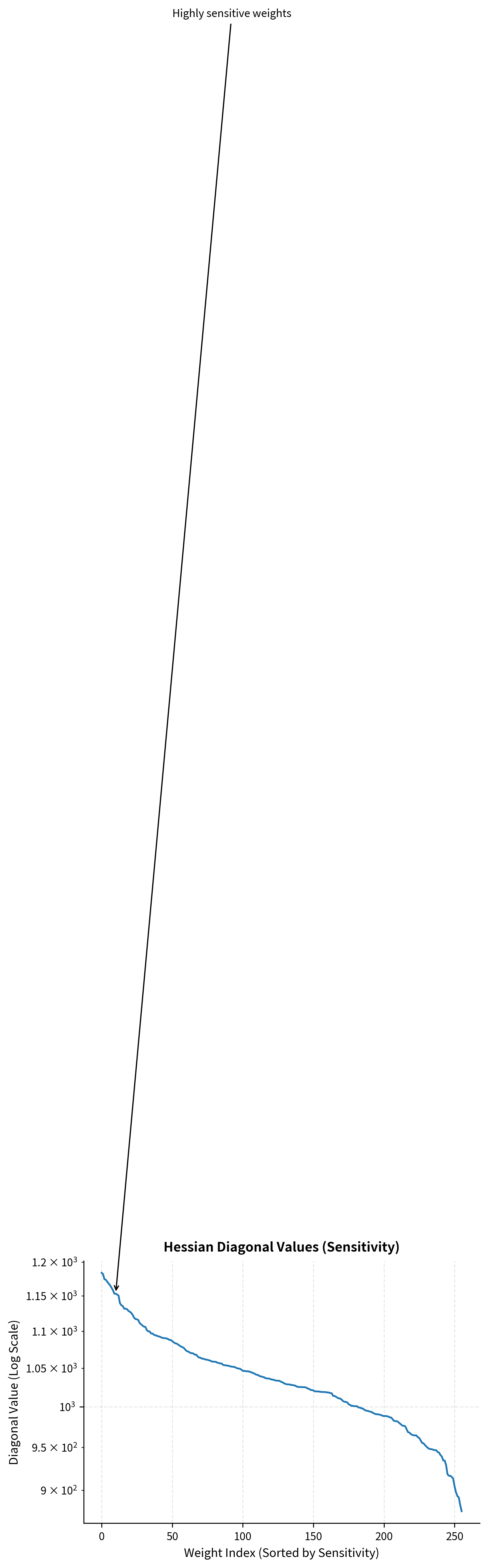
ActOrder (activation ordering) processes columns in decreasing order of their Hessian diagonal values . Weights with larger have greater impact on the output and are quantized first, when the most other weights are available for compensation.
The Hessian diagonal values reveal that the 'important' columns have much higher sensitivity (larger values) than the least important ones. Processing these sensitive columns first minimizes the accumulation of error.
ActOrder typically improves perplexity by 0.1-0.5 points at 4-bit precision, with the benefit more pronounced for smaller models where each weight matters more.
Perplexity Comparison
The ultimate test of quantization quality is model performance on downstream tasks. For language models, perplexity on held-out text provides a good proxy. Here's typical performance for GPTQ-quantized LLaMA models on WikiText-2:
| Model | FP16 PPL | GPTQ 4-bit PPL | Degradation |
|---|---|---|---|
| LLaMA-7B | 5.68 | 5.85 | +0.17 |
| LLaMA-13B | 5.09 | 5.20 | +0.11 |
| LLaMA-30B | 4.77 | 4.84 | +0.07 |
| LLaMA-65B | 4.53 | 4.58 | +0.05 |
The perplexity degradation shrinks with model size. Larger models have more redundancy and can better absorb quantization error. At 65B parameters, the difference between FP16 and GPTQ 4-bit is barely measurable on most benchmarks.
Limitations and Impact
GPTQ revolutionized LLM deployment by making aggressive quantization practical. A 65B parameter model that requires 130GB in FP16 fits in under 35GB with GPTQ 4-bit quantization. This brought state-of-the-art language models from server clusters to consumer GPUs.
However, GPTQ has several limitations worth understanding:
Calibration sensitivity. The quality of quantization depends on the calibration data. Models quantized with calibration data from one domain may perform poorly on another. For specialized applications (code generation, medical text), using domain-specific calibration data is important.
Computational cost. GPTQ quantization is significantly slower than naive round-to-nearest. Quantizing a 7B model takes around 10-30 minutes on a modern GPU, and the time scales superlinearly with model size due to the Hessian computations. This is acceptable for one-time quantization but makes GPTQ unsuitable for dynamic quantization during inference.
Layer-wise approximation. By optimizing each layer independently, GPTQ ignores how quantization errors compound across layers. A small error in early layers might be amplified by later layers. Methods like GPTQ don't account for this cross-layer interaction.
Activation quantization. GPTQ only quantizes weights, not activations. For inference on specialized hardware that requires both weight and activation quantization, additional techniques are needed.
Outlier sensitivity. The Hessian estimation can be skewed by outlier activations. As discussed in our chapter on INT8 quantization, transformer models sometimes produce extreme activation values that disproportionately influence the statistics. The dampening factor helps but doesn't fully solve this.
Despite these limitations, GPTQ remains one of the most effective post-training quantization methods for LLMs. Its combination of theoretical foundation (optimal error compensation) and practical efficiency (Cholesky-based updates) set the standard for weight quantization.
The success of GPTQ inspired subsequent work like AWQ (Activation-aware Weight Quantization), which we'll explore in the next chapter. AWQ takes a different approach by preserving important weights rather than compensating for errors, often achieving even better results on certain models.
Summary
GPTQ transforms weight quantization from a simple rounding problem into an optimization problem. By compensating for each weight's quantization error through updates to remaining weights, GPTQ achieves reconstruction error far below what naive quantization can manage.
The key elements that make GPTQ work are the Hessian matrix (capturing weight importance through input statistics), the optimal compensation formula (distributing error across correlated weights), and algorithmic optimizations (Cholesky factorization, column-wise processing) that make the approach tractable at scale.
For you, GPTQ means that 4-bit quantization is practical for production LLM deployment. Models lose minimal accuracy while fitting in a fraction of the original memory. The calibration data requirements and quantization time are modest costs for the dramatic efficiency gains.
Understanding GPTQ also provides insight into the broader space of quantization methods. The principle of error compensation, rather than pure rounding, appears in various forms across modern quantization techniques. Whether you're deploying a quantized model or developing new efficiency methods, the foundations established by GPTQ remain essential knowledge.
Quiz
Ready to test your understanding? Take this quick quiz to reinforce what you've learned about GPTQ.

Comments