

Discover GGUF format for storing quantized LLMs. Learn file structure, quantization types, llama.cpp integration, and deploying models on consumer hardware.

This article is part of the free-to-read Language AI Handbook
Choose your expertise level to adjust how many terms are explained. Beginners see more tooltips, experts see fewer to maintain reading flow. Hover over underlined terms for instant definitions.
GGUF Format
The quantization techniques we've explored so far, from INT8 to GPTQ and AWQ, represent powerful compression methods. However, a quantized model is only useful if you can actually run it. This is where theory meets practice, requiring both an efficient storage format and a capable inference engine. You need a file format that can store quantized weights efficiently and an inference engine that can execute them quickly. The GGUF format and its companion project llama.cpp have become the de facto standard for running large language models on consumer hardware, enabling everything from laptops to smartphones to run models that would otherwise require datacenter GPUs.
GGUF (GPT-Generated Unified Format) is a binary file format designed specifically for storing quantized neural network weights along with all the metadata needed to load and run them. Unlike generic serialization formats like PyTorch's .pt files or SafeTensors, GGUF was purpose-built for efficient CPU inference of transformer models. It supports a wide array of quantization schemes, from simple 4-bit integer quantization to sophisticated mixed-precision approaches, and packages everything into a single self-contained file.
From GGML to GGUF
The story of GGUF begins with GGML (Georgi Gerganov Machine Learning), a tensor library written in C that Georgi Gerganov created in 2022. Unlike frameworks such as PyTorch or TensorFlow that were designed for training on GPUs, GGML focused exclusively on inference and was optimized primarily for CPUs. This seemingly counterintuitive choice proved wise: while GPUs excel at parallel matrix operations, CPUs are available everywhere and can efficiently run quantized models that fit in system memory.
The original GGML library used a simple file format with a binary header followed by tensor data. Each model architecture had its own loading code, and metadata about the model (vocabulary, hyperparameters, tokenizer configuration) was stored in separate files or hardcoded into the loading routines. This worked, but it was fragile and didn't scale well as the community wanted to support more architectures.
In August 2023, the community introduced GGUF as a successor format. The key improvements:
- Self-contained metadata: All model information lives in a single file.
- Architecture agnostic design: The same format works for any supported architecture.
- Extensibility: New metadata fields can be added without breaking backward compatibility.
- Memory mapping: Tensor data can be accessed directly from disk without full loading.
- Alignment guarantees: Data is aligned for efficient memory access.
The transition wasn't instantaneous. For several months, you would see both .ggml and .gguf files floating around the community. Today, GGUF has essentially replaced GGML entirely, and the llama.cpp project only supports the newer format.
GGUF File Structure
A GGUF file consists of three main sections: a header, metadata key-value pairs, and tensor data. Understanding this structure helps when you need to inspect models, debug loading issues, or build your own tooling. The design philosophy behind this organization prioritizes both human readability during debugging and machine efficiency during loading: By separating the concerns into distinct sections, parsers can quickly validate a file, extract configuration without touching the weights, or memory-map only the tensor data for inference.
Header
The file begins with a fixed header that identifies it as GGUF and provides the counts needed to parse the rest. This header serves as both a validation mechanism and a roadmap for the parser: it tells parsers exactly how much data to expect in subsequent sections.
Offset  Size    Field
0       4       Magic number ("GGUF" = 0x46554747)
4       4       Version (currently 3)
8       8       Number of tensors
16      8       Number of metadata key-value pairs
Where:
- Offset: the byte position from the start of the file where each field begins (measured in bytes from position 0)
- Size: the number of bytes allocated for each field (1, 4, or 8 bytes depending on the data type)
- Field: a description of what information is stored at that location
- Magic number (0x46554747): a specific 4-byte sequence that spells "GGUF" in little-endian byte order. is used to quickly verify file type validity. When a parser reads these first four bytes and finds this exact sequence, it can be confident the file is a genuine GGUF file rather than some other format or corrupted data.
- Version (currently 3): the format version number. allows parsers to handle different format iterations while maintaining backward compatibility. When the format evolves to add new features or change how data is organized, the version number increments, signaling to parsers which set of rules to apply.
- Number of tensors: the total count of weight tensors stored in this file. tells parsers how many tensor definitions to expect in the tensor information section. Knowing this count upfront allows parsers to allocate appropriate data structures before reading tensor metadata.
- Number of metadata key-value pairs: the count of metadata entries following the header. indicates how many key-value pairs the parser must read before reaching tensor information. Like the tensor count, this enables efficient parsing by eliminating the need to scan for end markers.
The magic number lets tools quickly verify they're looking at a GGUF file. The version field allows the format to evolve while maintaining backward compatibility. Versions 1 and 2 had different alignment and encoding rules; version 3 is the current standard. This versioning strategy means that as the community discovers better ways to organize data or needs to support new quantization methods, the format can adapt without breaking existing files.
Metadata
Following the header, metadata is stored as a sequence of key-value pairs. This section contains all the information an inference engine needs to understand and execute the model, from basic architecture parameters to complete tokenizer vocabularies. Each pair consists of:
- A string key (UTF-8, length-prefixed)
- A type code indicating the value type
- The value itself
The supported value types include:
- Scalars: uint8, int8, uint16, int16, uint32, int32, uint64, int64, float32, float64, bool
- String: UTF-8 encoded, length-prefixed
- Array: A type code, followed by a count, followed by that many values
GGUF defines a standard set of metadata keys with specific meanings. The most important ones include:
general.architecture: The model family (e.g., "llama", "falcon", "mpt")general.name: Human-readable model namegeneral.quantization_version: Version of the quantization process{arch}.context_length: Maximum sequence length{arch}.embedding_length: Hidden dimension size{arch}.block_count: Number of transformer layers{arch}.attention.head_count: Number of attention heads{arch}.attention.head_count_kv: Number of key-value heads (for GQA)tokenizer.ggml.model: Tokenizer type ("llama", "gpt2", etc.)tokenizer.ggml.tokens: Array of vocabulary tokenstokenizer.ggml.scores: Token scores for SentencePiece modelstokenizer.ggml.token_type: Type of each token (normal, special, etc.)
This metadata allows the inference engine to configure itself entirely from the file contents. There is no need for separate configuration files or hardcoded model-specific logic. The self-describing nature of GGUF means that a single inference engine can load any supported model architecture without prior knowledge of its specific configuration.
Tensor Information
After the metadata comes information about each tensor. This section acts as an index or table of contents for the actual weight data, providing everything needed to locate and interpret each tensor without having to parse the tensor data itself. For each tensor, the file stores:
- Name (string)
- Number of dimensions
- Dimensions array
- Data type (quantization format)
- Offset into the data section
Note that this section contains only tensor metadata, not the actual weights. The tensor data comes later, after alignment padding. This separation is deliberate and crucial for efficient loading. By placing tensor metadata before the data, parsers can build a complete map of all tensors, allocate memory appropriately, and then load only the tensors actually needed for inference.
Tensor Data
The final section contains the actual tensor data, aligned to a specified boundary (typically 32 bytes) for efficient memory-mapped access. When loading a GGUF file, inference engines can memory-map this section directly rather than copying the data into newly allocated memory. This dramatically reduces loading time for large models. Memory mapping is particularly powerful because it allows the operating system to manage which portions of the model are actually resident in RAM, enabling inference on models that might not entirely fit in available memory.
The tensor data is stored in the quantized format specified in the tensor information section. Different tensors can use different quantization formats within the same file, enabling mixed-precision approaches where attention weights might use higher precision than feed-forward layers. This flexibility is essential for optimizing the quality-size tradeoff, as different parts of a model have different sensitivities to quantization error.
Quantization Types
GGUF supports an extensive array of quantization schemes. Understanding the naming conventions and trade-offs helps you choose the right model variant for your hardware constraints. The quantization landscape in GGUF has evolved considerably since the format's introduction, with newer methods achieving better quality at the same bit widths through more sophisticated compression strategies.
Naming Convention
Quantization types in GGUF follow a naming pattern: Q{bits}_{variant}. The bits indicate the average bits per weight, and the variant specifies the quantization method. This naming convention makes it straightforward to compare options and understand roughly what to expect from each format in terms of file size and quality.
The basic quantization types:
-
Q4_0: Simple 4-bit quantization with a single scale factor per block of 32 weights
-
Q4_1: 4-bit with both scale and minimum values per block
-
Q5_0: 5-bit quantization (4 bits + 1 extra bit per weight)
-
Q5_1: 5-bit with scale and minimum
-
Q8_0: 8-bit quantization, high quality but larger files K-quant methods, introduced in mid-2023, brought significant quality improvements. They use different block sizes and more sophisticated quantization schemes. The "K" designation indicates that these methods employ a key innovation in how they allocate quantization levels across the weight distribution.
-
Q2_K: Aggressive 2-bit quantization, smallest files but noticeable quality loss
-
Q3_K_S: 3-bit "small" variant, smaller files
-
Q3_K_M: 3-bit "medium", balanced
-
Q3_K_L: 3-bit "large", higher quality
-
Q4_K_S: 4-bit small, good balance of size and quality
-
Q4_K_M: 4-bit medium, the most popular choice for many users
-
Q5_K_S: 5-bit small
-
Q5_K_M: 5-bit medium, excellent quality
-
Q6_K: 6-bit, near-original quality
The K-quant methods improve on the basic Q4/Q5 formats by using non-uniform quantization. Rather than dividing the weight range evenly, they place more quantization levels where weights are densest. This approach recognizes that weight distributions in neural networks are not uniform: they tend to cluster around zero with long tails. By concentrating quantization levels where most weights actually lie, K-quant methods preserve more information with the same number of bits. They also use "super-blocks" that group multiple blocks together with shared statistics, further reducing overhead while maintaining accuracy.
I-Quant Methods
More recently, "importance matrix" (I-quant) methods have emerged:
- IQ1_S, IQ1_M: Extreme 1-bit quantization using importance weighting
- IQ2_XXS, IQ2_XS, IQ2_S, IQ2_M: Various 2-bit importance-weighted variants
- IQ3_XXS, IQ3_XS, IQ3_S, IQ3_M: 3-bit variants
- IQ4_NL, IQ4_XS: 4-bit with non-linear quantization
I-quant methods use calibration data to measure which weights have the most impact on model outputs, then allocate more precision to those weights. This connects to the ideas behind AWQ that we covered in the previous chapter, though implemented differently. The fundamental insight is the same: not all weights matter equally for model quality, so a smart quantization scheme should spend its limited precision budget where it counts most.
Comparing Quality vs Size
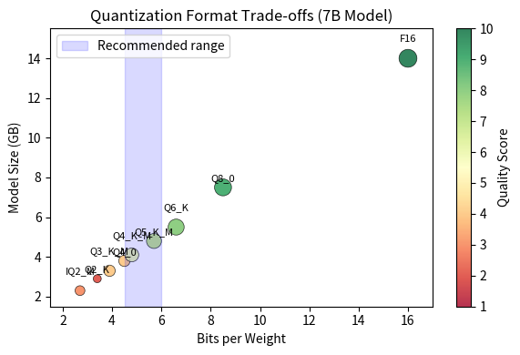
The practical trade-offs between quantization types can be substantial. The table below provides estimates for a 7 billion parameter model, showing how different quantization choices affect both storage requirements and expected quality.
| Type | Bits/Weight | Size (7B model) | Quality |
|---|---|---|---|
| F16 | 16.0 | ~14 GB | Original |
| Q8_0 | 8.5 | ~7.5 GB | Excellent |
| Q6_K | 6.6 | ~5.5 GB | Very good |
| Q5_K_M | 5.7 | ~4.8 GB | Good |
| Q4_K_M | 4.8 | ~4.1 GB | Good |
| Q4_0 | 4.5 | ~3.8 GB | Fair |
| Q3_K_M | 3.9 | ~3.3 GB | Moderate |
| Q2_K | 3.4 | ~2.9 GB | Poor |
| IQ2_M | 2.7 | ~2.3 GB | Fair for size |
The "bits per weight" column includes overhead from scale factors and other metadata, so it's always slightly higher than the base quantization level. This overhead varies by method because different quantization schemes store different amounts of auxiliary information alongside the quantized weights. For most use cases, Q4_K_M offers an excellent balance: models are about 4× smaller than FP16 with quality losses that are often imperceptible in practice. This sweet spot makes Q4_K_M the default recommendation for users who want to run large models on consumer hardware while maintaining reasonable quality.
llama.cpp Integration
llama.cpp is the reference implementation for GGUF inference. Originally created to run LLaMA models on MacBooks, it has evolved into a comprehensive inference engine supporting dozens of architectures.
Architecture
llama.cpp is written in C/C++ with a focus on portability and performance. - No external dependencies: Everything needed is included in the source tree
- Platform abstraction: Runs on Windows, macOS, Linux, iOS, Android
- Hardware acceleration: Supports Metal (Apple), CUDA (NVIDIA), ROCm (AMD), Vulkan, OpenCL
- SIMD optimization: Hand-tuned kernels for AVX, AVX2, AVX-512, NEON
The inference pipeline follows a straightforward flow:
- Memory-map the GGUF file
- Parse metadata to determine architecture and configuration
- Set up compute context based on available hardware
- Create the computation graph for forward passes
- Execute inference, processing one token at a time
Supported Architectures
Beyond LLaMA, llama.cpp now supports an extensive - LLaMA family: LLaMA, LLaMA 2, LLaMA 3, Code Llama
- Mistral family: Mistral, Mixtral (including MoE support)
- Other open models: Falcon, MPT, GPT-NeoX, Qwen, Phi, Gemma, RWKV
- Embedding models: BERT, Nomic-Embed
Each architecture is implemented as a set of layer definitions that map to the metadata stored in GGUF files. When you load a GGUF model, llama.cpp reads the general.architecture field and instantiates the appropriate layer stack.
Quantization with llama.cpp
The llama.cpp project includes a tool called quantize that converts models between formats. Starting from a full-precision GGUF file (typically converted from Hugging Face format), you can produce any of the quantization variants:
For I-quant methods, you can provide an importance matrix derived from calibration data:
The importance matrix is generated by running sample text through the model and measuring gradient magnitudes, similar to the calibration process in AWQ.
Working with GGUF Files
Let's explore GGUF files programmatically. While llama.cpp's command-line tools are useful, Python libraries provide a more interactive way to inspect and manipulate these files.
Now let's create a function to read and display the metadata from a GGUF file:
To demonstrate this parser, we need a GGUF file. Let's use the gguf Python library to create a simple one:
The output displays the GGUF file header information and metadata we just created, showing version 3 (the current GGUF standard), along with the model configuration we defined. The metadata fields show the model configuration: context length of 2048 tokens, embedding dimensions of 256, 4 transformer blocks, and 8 attention heads. This demonstrates how GGUF files package all necessary model information into a single self-contained format. In a real model, you would see many more metadata fields describing the full architecture configuration, including tokenizer information, feed-forward dimensions, and architecture-specific parameters.
Using the gguf Library
The gguf library provides higher-level APIs for reading GGUF files:
The inspection output summarizes the GGUF file structure, showing the architecture type (demo), key model parameters (context length, embedding size, block count, attention heads), and tensor statistics (total size and quantization types). This provides a quick overview of what's stored in the file and how the model is configured. The total tensor size of approximately 0.25 MB reflects our small demonstration model with a single 256×256 weight matrix.
Inspecting Tensor Information
Let's look more closely at the tensors stored in a GGUF file:
The tensor details reveal the structure and storage requirements of each weight tensor in the file. Our demo shows a single FP32 tensor of shape [256, 256], consuming about 0.25 MB (256 × 256 × 4 bytes per float32). In a real quantized model, you would see multiple quantization types used strategically. For example, embedding layers often use Q8_0 for better quality since they directly impact token representations, while most attention and feed-forward network (FFN) layers use Q4_K_M for efficiency since the quality loss is minimal for these layers.
Converting Models to GGUF
A common workflow is converting a Hugging Face model to GGUF format. The llama.cpp repository includes conversion scripts for this purpose. Here's the conceptual process:
The conversion process reads the model weights from Hugging Face's safetensors format, reorganizes them according to GGUF conventions, and writes out the new file with all necessary metadata extracted from the model's configuration.
For models not yet supported by llama.cpp, you may need to write custom conversion code. The key is mapping the model's weight names to the expected GGUF tensor names:
The conversion examples demonstrate how HuggingFace tensor names map to GGUF's standardized naming conventions. Layer-specific weights transform from HuggingFace's nested structure (model.layers.N.component) to GGUF's flattened block-based naming (blk.N.component). For instance, model.layers.0.self_attn.q_proj.weight becomes blk.0.attn_q.weight. Model-level tensors like embeddings (token_embd.weight) and output layers (output.weight) use fixed names without layer indices. This consistent naming allows llama.cpp to load any LLaMA-architecture model without architecture-specific code, as the inference engine can locate weights by their standardized names.
Running Inference with llama.cpp Python Bindings
While llama.cpp is primarily a C++ project, Python bindings are available through the llama-cpp-python package. This makes it easy to use GGUF models from Python:
The key parameters when loading a model include:
- n_ctx: The context window size. Larger contexts require more memory for the KV cache.
- n_threads: Number of CPU threads. Usually set to the number of physical cores.
- n_gpu_layers: How many layers to offload to GPU. Partial offloading helps when VRAM is limited.
- n_batch: Batch size for prompt processing. Larger batches are faster but use more memory.
For GPU acceleration, llama.cpp supports multiple backends. The choice depends on your hardware:
Memory Requirements
Understanding memory requirements helps you choose the right quantization level for your hardware. The total memory needed includes:
- Model weights: Size depends on quantization
- KV cache: Grows with context length and batch size
- Computation buffers: Temporary storage for intermediate activations weight memory requirements, we use a straightforward calculation. Given the number of parameters and the bits per weight for a specific quantization type, we can compute the total storage needed. The core idea is simple: each parameter requires a certain number of bits to store, and we convert this total bit count first to bytes, then to gigabytes for human-readable output. The formula converts parameter count to total bits, then to bytes, then to gigabytes:
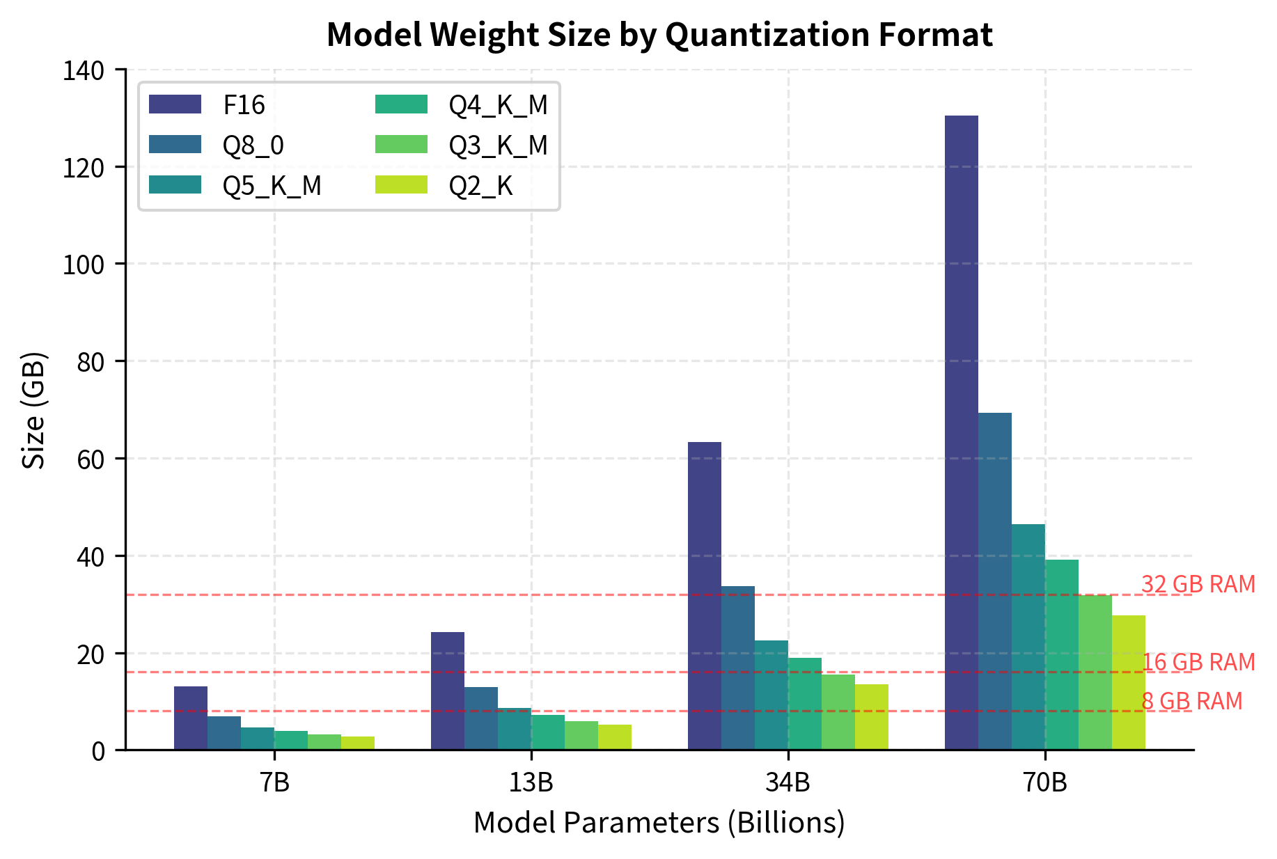
The model size estimates show how quantization dramatically reduces storage requirements. A 7B parameter model in FP16 format requires about 14 GB, while Q4_K_M quantization reduces this to approximately 4.1 GB (a 3.4× reduction), making it feasible to run on consumer hardware with 8-16 GB of RAM. Moving to more aggressive quantization like Q2_K further reduces size to 2.9 GB, though at the cost of model quality. These estimates cover only the model weights and don't include the KV cache, which can be substantial for long contexts. A 7B model with 4096 context length typically needs an additional 1-2 GB for the cache when using FP16 KV values, bringing total memory requirements to 5-6 GB for Q4_K_M models.
To understand how much memory the KV cache requires, we need to account for several factors working together: the number of layers storing caches, the size of each cache entry, the number of tokens being cached, and the precision of the cached values. During inference, the model stores attention keys and values for all tokens in the context window, meaning this cache grows linearly with sequence length. This calculation helps determine whether a model will fit in available memory, as the KV cache can sometimes rival or even exceed the model weights in size for very long contexts.
The KV cache memory requirement can be estimated using:
where:
- is the number of transformer layers in the model. Each layer maintains its own key-value cache, storing the computed attention keys and values so they don't need to be recomputed for previously processed tokens.
- is the hidden dimension size (embedding length). It determines the size of each cached vector, as every cached key and value is a vector of this dimensionality.
- is the context length (maximum sequence length). It represents how many token positions we need to cache, with longer contexts requiring proportionally more memory.
- is the number of bits per KV value (16 for FP16, 8 for Q8, etc.). It controls the precision of cached values, where lower precision reduces memory but may affect numerical accuracy.
- is a factor accounting for both key and value caches (we store one cache for keys and one for values)
- is the conversion factor from bits to bytes
- is the conversion factor from bytes to gigabytes
The formula computes total memory by first calculating the number of bits needed, then converting to gigabytes through two unit conversions. Let's examine each component step by step to build intuition for how these factors combine.
The numerator calculates the total number of bits required:
This product can be understood in stages, building up from basic quantities to the final bit count. First, gives us the total number of scalar values in one cache (either keys or values). Here's why: each of the layers needs to cache tokens, and each token's representation is a -dimensional vector. Multiplying these together gives the total count of individual numbers we need to store for one cache. Since we need separate caches for both keys and values, we multiply by 2. Finally, multiplying by converts from the count of values to the count of bits, since each value requires bits of storage.
The denominator performs two sequential unit conversions:
Dividing by 8 converts bits to bytes (8 bits = 1 byte), and dividing by converts bytes to gigabytes (1 GB = bytes = 1,073,741,824 bytes). These conversions happen in sequence, moving from bits to bytes to gigabytes, giving us a final result in units that are easy to compare against available system memory.
The factor of 2 is critical because attention mechanisms require separate caches for keys and values at each layer. Without this factor, we would only be accounting for one of the two caches. The key cache stores the projections used to match against queries, while the value cache stores the information that gets retrieved once a match is found.
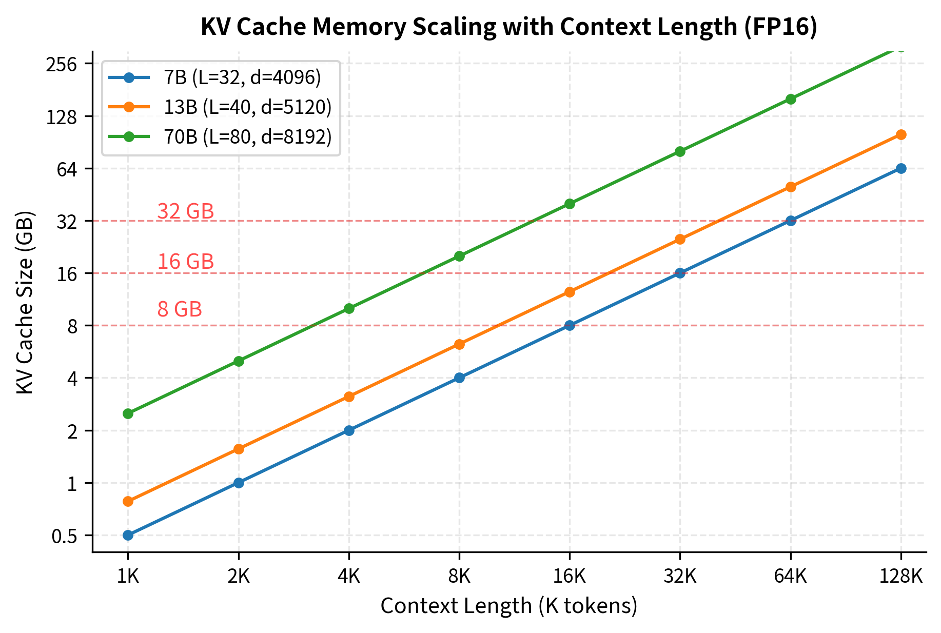
The multiplicative structure of this formula has important implications for system design. Doubling any factor (layers, dimension, or context length) doubles the memory requirement. This linear scaling means that extending context windows comes with a predictable but substantial memory cost. For instance, moving from a 4K to an 8K context doubles the KV cache requirement, while moving to 32K contexts requires 8× more memory for the cache alone.
Let's see how this formula works in practice with a concrete example. Consider a typical 7B parameter model with the following specifications:
- transformer layers
- hidden dimensions
- context length (maximum sequence length)
- bits per value (FP16 precision)
Substituting these values into our formula:
This calculation shows that the KV cache requires approximately 2 GB of additional memory beyond the model weights themselves. To understand why this result makes sense, let's break down the calculation into clear stages that build intuition for the memory requirements.
First, we calculate the total number of values that need to be cached. This includes both keys and values across all layers and all token positions:
This tells us we need to store over 1 billion individual numbers. The sheer scale of this count illustrates why the KV cache consumes so much memory. Next, we convert this count to bytes. Since each value uses FP16 precision (16 bits = 2 bytes), we multiply by 2:
Finally, we convert bytes to gigabytes by dividing by :
The multiplicative structure of this formula reveals an important scaling property. Since context length appears as a direct multiplier in the numerator, doubling the context length doubles the memory requirement. This linear scaling means that extending context windows comes with a predictable but substantial memory cost.
For example, if a model requires 2 GB of KV cache at 4K context:
- At 8K context,
- At 16K context,
- At 32K context,
This makes KV cache management critical for long-context applications. Moving from 4K to 32K contexts requires 8× more memory for the cache alone, which can quickly exceed available RAM or VRAM on consumer hardware. This scaling behavior explains why many long-context models employ specialized techniques like sliding window attention or sparse attention patterns to limit KV cache growth.
Limitations and Practical Considerations
GGUF and llama.cpp have made local LLM inference remarkably accessible, but several limitations are worth understanding.
Quality degradation at low bit widths remains the fundamental challenge. While Q4_K_M preserves most model capabilities for many tasks, aggressive quantization such as Q2_K or IQ2 causes noticeable degradation, especially for tasks requiring precise factual recall or complex reasoning. The impact varies by model architecture and size. Larger models tolerate quantization better because they have more redundancy in their representations.
CPU inference is slower than GPU inference, sometimes by an order of magnitude or more. For a 7B model, you might see 20-30 tokens per second on a modern CPU versus 80-100+ tokens per second on a mid-range GPU. This is acceptable for interactive use but can be limiting for batch processing. llama.cpp's GPU support has improved dramatically, but it still trails dedicated inference frameworks like vLLM for high-throughput serving.
Memory bandwidth often bottlenecks performance more than compute. Modern CPUs and GPUs can perform calculations faster than they can load weights from memory. This is why quantization helps. Moving from FP16 to Q4 not only reduces memory footprint by 4×, but also speeds up inference by roughly 2-3× because you are loading fewer bytes. Techniques like model sharding and layer-wise loading can help when models don't fit in memory, but they come with performance penalties.
Not all architectures are equally supported. While llama.cpp covers the major model families, newer or more exotic architectures may lag behind. The pace of new model releases means that quantized versions sometimes are not available immediately. The community-driven nature of llama.cpp means popular models get support quickly, but niche architectures may require custom work.
Tokenizer fidelity can be an issue when converting models. GGUF stores tokenizer information in its metadata, but subtle differences in how tokenizers handle edge cases can cause divergence from the original model's behavior. This is usually minor but can affect reproducibility for certain prompts.
Summary
GGUF has become the standard format for distributing and running quantized language models on consumer hardware. Its design priorities (self-contained metadata, efficient memory mapping, and flexible quantization support) make it well-suited for the diverse ecosystem of local LLM deployment.
The quantization options within GGUF span from near-lossless Q8_0 to aggressive IQ2 methods, with Q4_K_M emerging as the sweet spot for most users. The K-quant methods brought meaningful quality improvements over the original simple quantization schemes, and importance-based methods continue to push the frontier of what's possible at extreme compression levels.
llama.cpp provides the inference engine that brings GGUF models to life. Its CPU-first design with optional GPU acceleration means the same model file can run across a remarkable range of hardware, from smartphones to workstations. The Python bindings through llama-cpp-python make it easy to integrate GGUF models into applications.
Understanding GGUF empowers you to make informed choices about model variants, troubleshoot loading issues, and even create custom tooling for your specific needs. As we'll see in upcoming chapters on speculative decoding and inference serving, these foundations in model formats and efficient inference become building blocks for more sophisticated deployment strategies.
Key Parameters
The key parameters for working with GGUF models and llama.cpp:
- n_ctx: Context window size. Determines maximum sequence length the model can process.
- n_threads: Number of CPU threads to use for inference.
- n_gpu_layers: Number of transformer layers to offload to GPU (0 for CPU-only, -1 for all layers).
- n_batch: Batch size for prompt processing, affecting memory usage and throughput.
- tensor_split: Distribution of layers across multiple GPUs when using multi-GPU setups.
Quiz
Ready to test your understanding? Take this quick quiz to reinforce what you've learned about the GGUF format and efficient model inference.

Comments