LoRA Hyperparameters: Rank, Alpha & Target Module Selection

In the previous chapters, we established the mathematical foundation of LoRA and walked through its implementation. You now understand that LoRA introduces trainable low-rank matrices $A$ and $B$ to approximate weight updates without modifying the original model. But a critical question remains: how do you choose the hyperparameters that govern LoRA's behavior?

The hyperparameters you select fundamentally shape the trade-off between adaptation capacity and efficiency. A rank that's too low might not capture the complexity your task requires; a rank that's too high wastes compute and memory while potentially overfitting. Similarly, choosing which layers to adapt and how to scale their contributions can mean the difference between a well-adapted model and one that fails to generalize.

This chapter provides practical guidance for configuring LoRA based on empirical findings and intuition about what each hyperparameter controls.

The rank $r$ is LoRA's most important hyperparameter. It determines the dimensionality of the low-rank decomposition and directly controls the number of trainable parameters introduced. Understanding rank requires thinking carefully about what these low-rank matrices actually represent: they define a compressed subspace within which all adaptation must occur. A higher rank provides a richer, more flexible subspace capable of capturing more nuanced transformations, while a lower rank constrains the adaptation to simpler patterns that can be expressed with fewer degrees of freedom.

Recall from our discussion of LoRA mathematics that for a weight matrix $W \in \mathbb{R}^{d_{out} \times d_{in}}$, LoRA introduces:

where:

• $\Delta W$: the low-rank update matrix that captures all task-specific modifications to the original weights
• $B$: the up-projection matrix ($\in \mathbb{R}^{d_{out} \times r}$), which maps from the compressed rank-$r$ space back to the output dimension
• $A$: the down-projection matrix ($\in \mathbb{R}^{r \times d_{in}}$), which projects the input into the compressed rank-$r$ space

The fundamental insight here is that the product $BA$ can only produce matrices of rank at most $r$, regardless of how large $d_{in}$ and $d_{out}$ might be. This means we are implicitly assuming that the difference between what the pre-trained model computes and what we need for our specific task can be well-approximated by a low-rank transformation. This assumption is surprisingly valid in practice, as we will see.

Since the adapter consists of matrices $A$ ($r \times d_{in}$) and $B$ ($d_{out} \times r$), the total parameter count is the sum of their elements. To understand this concretely, consider that matrix $A$ has $r$ rows and $d_{in}$ columns, yielding $r \times d_{in}$ individual learnable parameters. Similarly, matrix $B$ has $d_{out}$ rows and $r$ columns, contributing $d_{out} \times r$ parameters. The number of trainable parameters per adapted weight matrix is therefore:

where:

• $\text{params}$: the total count of trainable parameters for the adapter
• $r$: the rank hyperparameter, the single value that controls the capacity of the entire adaptation
• $d_{out}$: the output dimension of the layer being adapted
• $d_{in}$: the input dimension of the layer being adapted

This formula reveals an elegant property: the parameter count scales linearly with rank. Doubling the rank exactly doubles the number of trainable parameters. It also scales linearly with the sum of dimensions rather than their product, which is the key insight that makes LoRA so efficient. For a square weight matrix where $d_{in} = d_{out} = d$, the original weight matrix has $d^2$ parameters while LoRA adds only $2rd$ parameters, a savings factor of $\frac{d}{2r}$.

Let's examine how rank affects parameter counts for typical transformer dimensions. This analysis will make concrete the dramatic parameter savings that LoRA provides across different model scales.

The parameter efficiency is striking and reveals why LoRA has become so popular for resource-constrained fine-tuning. For a 4096-dimensional model (like LLaMA-7B's hidden dimension), rank 16 uses about 0.8% of the parameters compared to full fine-tuning. This represents a reduction of more than 100x in the number of parameters that must be stored, optimized, and potentially distributed across training runs. This efficiency is why LoRA enables fine-tuning on consumer hardware: where full fine-tuning of a 7B parameter model might require multiple high-end GPUs, LoRA adaptation can often be accomplished on a single GPU with 16GB or even less memory.

Research and practitioner experience have converged on general guidelines that provide useful starting points. These recommendations emerge from extensive experimentation across diverse tasks and model architectures:

• Rank 4-8: Suitable for simple classification tasks, sentiment analysis, and tasks where the pre-trained model already performs reasonably well. At these ranks, you are making only subtle adjustments to the model's behavior, which is often sufficient when the pre-training distribution closely matches your target domain.
• Rank 16-32: The sweet spot for most instruction tuning and domain adaptation tasks. These ranks provide enough capacity to learn new behavioral patterns while remaining extremely parameter-efficient.
• Rank 64-128: Appropriate for complex tasks requiring significant behavior changes, multilingual adaptation, or when data is abundant. Here, you have capacity comparable to more substantial model modifications.
• Rank 256+: Rarely necessary; consider whether full fine-tuning might be more appropriate. At these ranks, you are approaching the parameter counts where the low-rank assumption provides diminishing benefits.

The original LoRA paper found that even rank 4 achieved competitive results on many tasks, suggesting that the update matrices for adapting pre-trained models often have low intrinsic dimensionality. This finding suggests that the space of useful adaptations is fundamentally lower-dimensional than the full weight space. This observation aligns with findings from the intrinsic dimensionality literature, which showed that fine-tuning can be effective in surprisingly low-dimensional subspaces. The implication is that pre-trained models have already learned rich, general representations, and task-specific adaptation primarily involves steering these existing capabilities rather than learning entirely new transformations.

The relationship between task complexity and optimal rank isn't strictly linear, and understanding the factors that influence this relationship helps you make informed decisions. Consider these factors when selecting rank:

Distance from pre-training distribution: Tasks requiring the model to behave very differently from its pre-training (e.g., adapting an English model to code generation) typically benefit from higher ranks. The model needs to learn substantial new patterns rather than slightly adjust existing ones. When the target behavior diverges significantly from what the model learned during pre-training, the required transformation has higher intrinsic dimensionality, necessitating a larger subspace for the adaptation.

Task-specific structure: Some tasks have inherently low-rank structure in the transformations they require. Classification problems that distinguish between a small number of categories often require fewer parameters than generation tasks that must produce diverse, nuanced outputs. A sentiment classifier essentially needs to learn a projection onto a low-dimensional decision boundary, while a creative writing assistant must capture subtle stylistic variations across an expansive output space.

Dataset size: With limited data (hundreds to low thousands of examples), lower ranks act as regularization, preventing overfitting. The constraint of a small subspace limits the model's ability to memorize training examples. Larger datasets can support higher ranks without memorization, as there is sufficient signal to guide learning in a higher-dimensional space.

Let's visualize how rank affects training dynamics using a simple simulation. This experiment creates a synthetic task with known intrinsic dimensionality and observes how different LoRA ranks perform in capturing the required transformation.

The simulation reveals important dynamics that generalize to real-world LoRA training. When the LoRA rank is below the true intrinsic dimensionality of the task (ranks 2 and 4 here), the model underfits and cannot fully capture the required transformation. The loss plateaus above the noise floor because the adapter simply lacks the capacity to represent the target function. Once the rank meets or exceeds the intrinsic dimensionality, convergence becomes similar, with higher ranks offering only marginal improvements. This demonstrates a key principle: beyond a certain point, additional rank provides diminishing returns, as the extra dimensions in the subspace go unused.

To understand this phenomenon more concretely, we can examine how well different ranks approximate a target low-rank transformation by measuring reconstruction error.

The visualization demonstrates a key insight: once the approximation rank reaches the target's true rank of 8, the reconstruction error drops to essentially zero. Additional rank beyond this point provides no benefit for this particular transformation. In practice, the "true rank" of a task-specific adaptation is unknown, but this principle explains why empirical tuning often reveals a clear knee in performance as rank increases.

The scaling factor $\alpha$ (alpha) is LoRA's second key hyperparameter. While rank determines the capacity of the adaptation, alpha controls the magnitude of the adaptation's contribution to the model's output. The adapted layer output $h$ sums the frozen pre-trained projection with the scaled low-rank update. As discussed in the LoRA mathematics chapter, the formula is:

where:

• $h$: the output vector of the adapted layer, combining both original and adapted computations
• $W$: the frozen pre-trained weight matrix that remains unchanged throughout training
• $x$: the input vector to the layer
• $Wx$: the output from the frozen pre-trained weights, representing the model's original behavior
• $BAx$: the update computed by the low-rank adapter, representing the task-specific modification
• $\alpha$: the scaling constant, a hyperparameter you set before training
• $r$: the rank of the LoRA matrices
• $\frac{\alpha}{r}$: the scaling factor that controls adaptation strength, computed from the ratio of alpha to rank
• $B$: the up-projection matrix that expands the low-rank representation
• $A$: the down-projection matrix that compresses the input

The ratio $\frac{\alpha}{r}$ scales the LoRA output before adding it to the original transformation. This ratio is the key quantity that determines how strongly the adaptation influences the model's predictions relative to its pre-trained behavior.

Alpha serves multiple purposes in the LoRA framework, each addressing a different practical concern:

Learning rate decoupling: By scaling the LoRA output, alpha allows you to use the same learning rate regardless of rank. Without this scaling, changing rank would require retuning the learning rate to achieve similar training dynamics. Consider what happens without the $\frac{\alpha}{r}$ factor: a rank-64 adapter would produce outputs with approximately 8 times the magnitude of a rank-8 adapter (due to the summation over more dimensions), completely changing the effective step size of gradient updates. The alpha scaling normalizes these differences.

Initialization stability: The $\frac{\alpha}{r}$ factor compensates for the fact that higher ranks produce outputs with higher variance (since more terms are summed). When matrix $A$ maps the input to $r$ dimensions and matrix $B$ maps those back to the output space, the variance of the resulting transformation scales roughly with $r$. The normalization by $r$ in the denominator counteracts this growth, helping maintain consistent output magnitudes across different rank choices.

Adaptation strength: Practically, alpha controls how much the LoRA adaptation influences the model's output relative to the frozen pre-trained weights. A larger alpha amplifies the adapter's contribution, allowing more aggressive modification of the model's behavior. A smaller alpha produces more conservative updates, keeping the model closer to its pre-trained state.

The ratio $\frac{\alpha}{r}$ determines the effective scaling and is the quantity that directly influences training behavior. Understanding this ratio helps you reason about different configuration choices. Common configurations include:

• $\alpha = r$: The most common choice, resulting in a scaling factor of 1. The LoRA update contributes with the same magnitude as if there were no explicit scaling. This provides a neutral baseline where the raw adapter output is added directly to the pre-trained computation.
• $\alpha = 2r$: Doubles the LoRA contribution, potentially accelerating adaptation but risking instability. With stronger updates, the model can adapt more quickly, but gradients may become large enough to cause training difficulties.
• $\alpha = r/2$: Halves the LoRA contribution, providing more conservative updates. This is useful when you want the model to retain more of its pre-trained behavior or when training with limited data where aggressive updates might lead to overfitting.

The LoRA-to-original ratio scales linearly with $\frac{\alpha}{r}$, exactly as the formula predicts. When alpha equals rank (16 in this example), the LoRA contribution has magnitude roughly proportional to the original output. Doubling alpha to 32 doubles this ratio, while halving alpha to 8 halves it. This linear relationship makes it straightforward to reason about how configuration changes will affect the model's behavior.

Selecting alpha in practice involves balancing several considerations. Here are guidelines based on common scenarios:

Default choice ($\alpha = r$): Start here. It provides balanced adaptation and has been validated across many tasks. The scaling factor of 1 means the adapter's influence is neither amplified nor diminished, giving you a clean baseline from which to adjust.

Higher alpha ($\alpha > r$): Consider when:

• You need faster adaptation with limited training steps, as stronger updates allow more learning per iteration
• The task requires strong deviation from pre-trained behavior, necessitating larger modifications
• You're using a low learning rate and want to compensate without changing the optimizer configuration

Lower alpha ($\alpha < r$): Consider when:

• Fine-tuning on limited data (extra regularization), where conservative updates help prevent the model from overwriting its useful pre-trained knowledge
• You want to preserve more of the pre-trained model's behavior, important for tasks where the original capabilities should remain intact
• Training is unstable with default settings, and reducing the adaptation strength can restore stable convergence

A common pattern in practice is to fix $\alpha = 16$ or $\alpha = 32$ regardless of rank. This means changing rank also changes the effective scaling, which can be useful: lower ranks get relatively stronger updates, partially compensating for their reduced capacity. This approach simplifies hyperparameter tuning by reducing the number of independent variables you need to consider.

With fixed alpha, lower ranks receive stronger per-parameter updates (higher effective scaling), while higher ranks receive more diluted updates. This implicit regularization can help: smaller adapters need more "strength" to achieve meaningful adaptation with their limited capacity. Conversely, larger adapters have enough parameters that each individual parameter can contribute less while still achieving substantial overall modification.

LoRA can be applied to any linear transformation in the model, but which layers you adapt significantly impacts both performance and efficiency. The choice of target modules determines which aspects of the model's computation you are modifying, and different choices lead to qualitatively different adaptations.

Recall from Part XII that transformer blocks contain several linear transformations, each playing a distinct role in the model's computation:

• Attention projections: $W_Q$, $W_K$, $W_V$ for queries, keys, and values; $W_O$ for output projection. These matrices control how the model attends to different parts of the input sequence and how it combines information across positions.
• Feed-forward networks: Two linear layers (up-projection and down-projection in standard architectures, plus gate projection in gated architectures like SwiGLU). These layers transform each token's representation independently, storing and retrieving factual knowledge.

Each of these has different roles and different responses to LoRA adaptation. Adapting attention layers primarily affects how the model routes and combines information, while adapting feed-forward layers affects what information is stored and retrieved at each position.

The original LoRA paper primarily experimented with attention weight matrices and found that adapting $W_Q$ and $W_V$ worked well for many tasks. This focus on attention was partly practical, as it kept parameter counts low, and partly theoretical, as attention mechanisms are thought to be more task-specific than the general-purpose transformations in feed-forward layers. However, subsequent work has explored broader patterns and found that different tasks benefit from different targeting strategies.

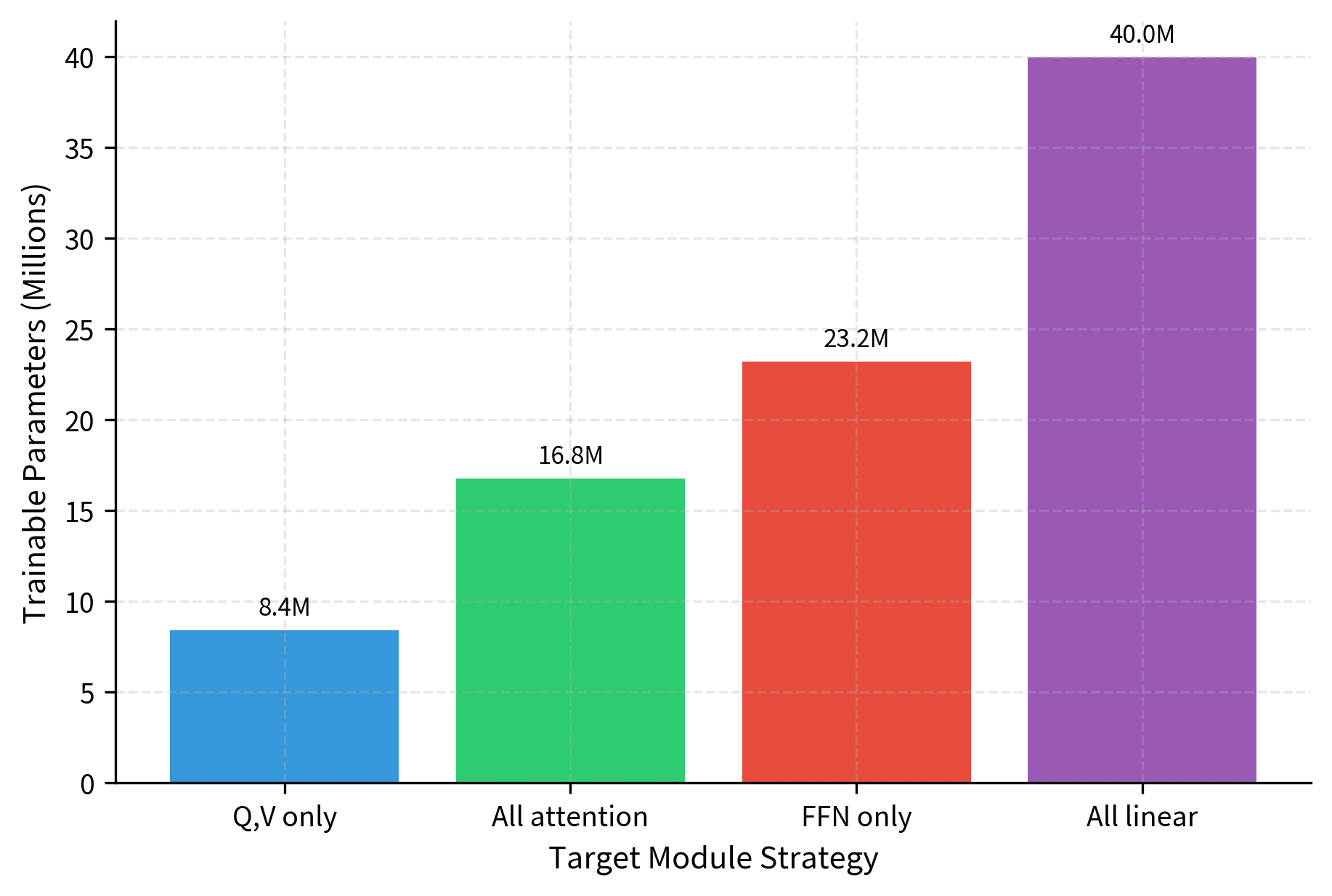
The visualization highlights the trade-off between adaptation depth and parameter efficiency. While attention-only strategies remain extremely lightweight, including feed-forward networks (All Linear) increases the parameter count significantly, though it remains a small fraction of the total model size. Notice that FFN-only adaptation actually uses more parameters than all-attention adaptation, because the feed-forward intermediate dimension (11008 in this example) is much larger than the hidden dimension (4096).

Choosing which modules to target requires balancing task requirements with computational constraints. Here are guidelines organized by strategy:

Attention-only (Q, V or all attention): Start here for most tasks. Attention layers determine how information flows between tokens, making them highly influential for task adaptation. When you modify query and value projections, you change what the model looks for in the input and what it extracts from attended positions. The original LoRA paper found Q and V sufficient for many tasks, though including K and O can help for more complex adaptations that require modifying how keys are computed and how attended information is projected back to the residual stream.

Feed-forward layers: These serve as "memory" in transformers, storing factual and procedural knowledge learned during pre-training. Research has shown that specific factual associations are often localized in particular feed-forward layers. Adapting FFN layers becomes important when:

• Your task requires new factual knowledge not present in the pre-training data
• You're adapting to a significantly different domain with domain-specific terminology or conventions
• Attention-only adaptation isn't achieving desired performance, suggesting the limitation lies in what knowledge is being retrieved rather than how information flows

All linear layers: Most comprehensive but also most parameter-heavy. Use when:

• You have abundant training data sufficient to support the increased capacity
• The task requires substantial behavioral changes across multiple dimensions
• You've validated that simpler strategies underperform and the extra parameters are justified

Let's examine how different targeting strategies affect model behavior in practice by comparing concrete parameter counts.

Focusing on Q and V projections keeps the trainable parameter count under 0.1% of the total model size, representing extreme parameter efficiency. Expanding to all attention matrices doubles this footprint, while including FFN layers (All Linear) increases it nearly five-fold, though still remaining below 0.5%. Even the most comprehensive strategy adapts less than one percent of the model's parameters, highlighting LoRA's fundamental efficiency advantage over full fine-tuning.

An advanced strategy allows different ranks for different layer types. This recognizes that attention and FFN layers may have different intrinsic dimensionalities for adaptation: the patterns needed to modify attention behavior might be simpler (lower rank) than those needed to inject new knowledge into feed-forward layers (higher rank).

By allocating higher ranks to the FFN layers (which often require more capacity to store new knowledge) and lower ranks to attention layers (where steering behavior is often simpler), this mixed strategy optimizes the parameter budget. The total count lies between the attention-only and all-linear approaches, providing a middle ground that acknowledges the different roles these components play.

LoRA dropout applies dropout to the LoRA branch during training, providing regularization that can improve generalization. Unlike standard dropout which is applied throughout the network, LoRA dropout specifically targets the adapter pathway, leaving the frozen pre-trained computation unaffected.

Dropout is applied after the first matrix multiplication in the LoRA path, introducing stochastic noise during the forward pass:

where:

• $h$: the layer output, combining frozen and adapted computations
• $W$: the frozen pre-trained weight matrix
• $x$: the input vector
• $\alpha$: the scaling constant
• $r$: the rank hyperparameter
• $B$: the up-projection matrix
• $A$: the down-projection matrix
• $\text{Dropout}(\cdot)$: the dropout operation that randomly zeros elements
• $Ax$: the intermediate low-rank projection, the target of dropout

During training, elements of $Ax$ are randomly zeroed with probability $p$, and the remaining elements are scaled by $\frac{1}{1-p}$ to maintain expected values. This rescaling ensures that the expected output magnitude remains the same whether dropout is applied or not. At inference time, dropout is disabled and the full LoRA contribution is used, giving consistent and deterministic predictions.

As we discussed in Part VII on dropout, this prevents co-adaptation of features and acts as an ensemble of subnetworks. Each training step effectively uses a different random subset of the adapter's capacity, forcing the model to learn robust representations that don't rely on any single pathway. In the LoRA context, it prevents the low-rank adaptation from overfitting to training examples by ensuring that the adaptation remains effective even when parts of it are randomly disabled.

Common dropout rates for LoRA range from 0.0 to 0.1, with several factors influencing the choice:

• Dataset size: Smaller datasets benefit from higher dropout (0.05-0.1) to prevent overfitting, as the regularization helps the model generalize from limited examples. Large datasets may need little to no dropout, as the abundance of training signal naturally prevents memorization.
• Rank: Higher ranks have more capacity to overfit, making dropout more valuable. The additional parameters in a high-rank adapter provide more opportunities for the model to memorize training examples. Very low ranks (4 or less) often work fine without dropout, as their limited capacity already provides implicit regularization.
• Task complexity: Simple classification tasks typically need less regularization than generation tasks. Generation requires the model to produce diverse, coherent outputs, making it more susceptible to subtle forms of overfitting that dropout can help prevent.

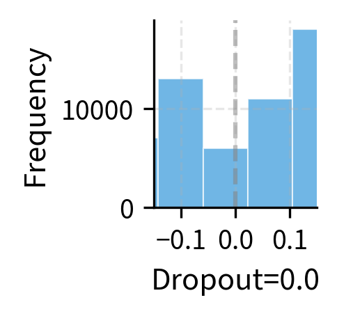
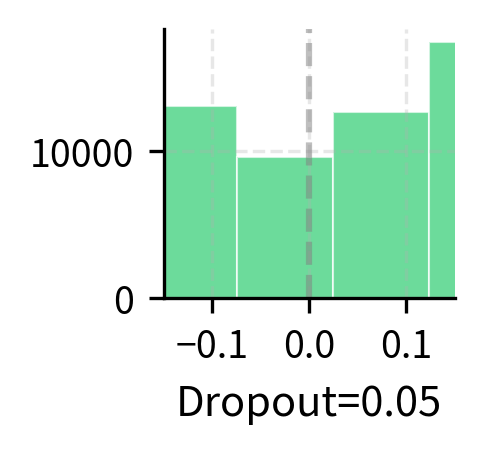
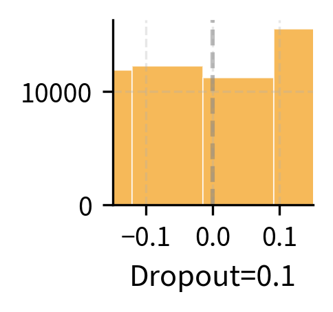
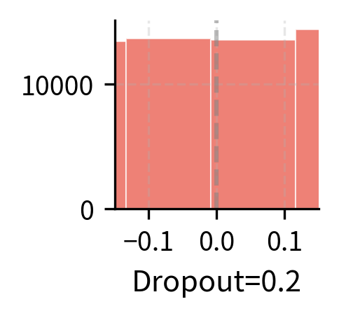
Higher dropout rates introduce more variance in training, which can help prevent overfitting but may also slow convergence. The output variance scales with dropout, as random subsets of the LoRA capacity are used for each forward pass. Notice that at 20% dropout, the output variance is substantial, meaning the model receives different signals on different training steps. This stochasticity encourages learning representations that are robust to partial information, but too much variance can make training unstable.

LoRA dropout interacts with rank and alpha in subtle ways that merit careful consideration:

Rank-dropout interaction: With higher ranks, each forward pass uses a larger absolute number of features even at the same dropout rate. A rank-64 adapter with 10% dropout still uses roughly 58 features on average, while a rank-8 adapter uses only about 7. This means dropout is relatively more aggressive for low-rank configurations. A 10% dropout on a rank-4 adapter leaves only about 3.6 features active on average, which may severely limit the adapter's effective capacity. Consider using lower dropout rates with lower ranks.

Alpha-dropout interaction: Dropout doesn't change the expected value of the output due to the rescaling, but it does change the gradient variance. Each training step sees a different random subset of the network, leading to gradients that fluctuate around their expected values. Higher alpha amplifies both the mean and variance of gradients, so combining high alpha with high dropout can lead to noisy training. If you observe training instability with high alpha, reducing dropout may help restore smooth convergence.

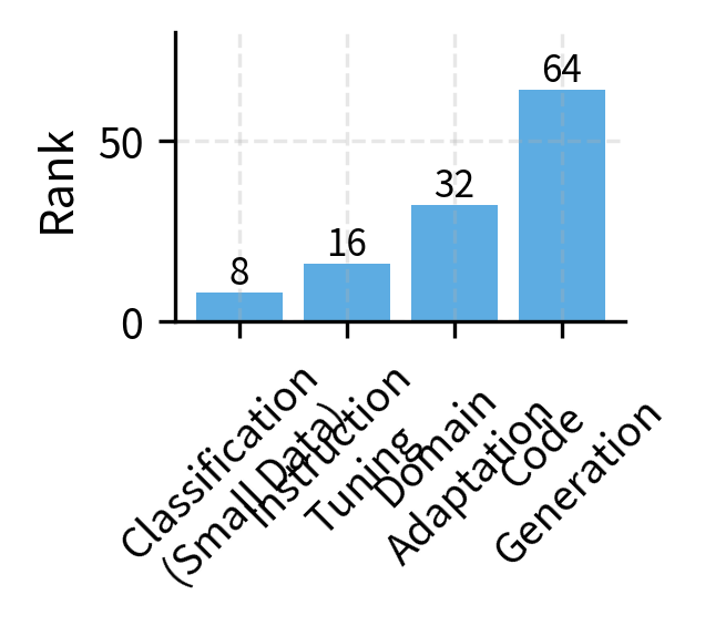
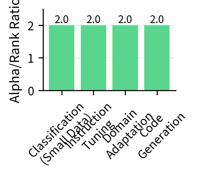
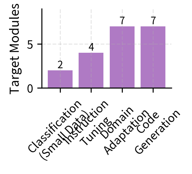
Let's consolidate these guidelines into practical configurations for common scenarios. These recipes represent starting points based on accumulated practitioner experience, though optimal configurations may vary based on your specific model, data, and requirements.

Here's how these hyperparameters come together in practice, demonstrating the configuration structure you would use with the PEFT library.

The configuration targets all attention matrices with rank 16 and alpha 32, creating a scaling factor of 2. This amplified scaling helps the adapter make meaningful contributions despite its small parameter count. The modest dropout of 0.05 provides light regularization without significantly slowing convergence. This setup balances capacity with stability, making it a robust starting point for instruction tuning tasks.

When optimal values aren't clear from guidelines, systematic search can help. The key is to search efficiently, focusing computational resources on the hyperparameters most likely to impact performance.

Not all hyperparameters deserve equal search effort. Prioritize in this order:

1. Target modules: The biggest impact on both performance and efficiency. Start with attention-only, expand if needed. This decision fundamentally changes what aspects of the model you are adapting.
2. Rank: Affects capacity directly. Search powers of 2 (4, 8, 16, 32) as these are natural scales for the problem.
3. Alpha: Usually set relative to rank. Try $\alpha = r$, then $\alpha = 2r$ if more adaptation strength is needed.
4. Dropout: Fine-tune last. Start with 0.05, increase to 0.1 if overfitting, decrease to 0 if underfitting.

A balanced search with 36 configurations is manageable for most projects. Each configuration trains quickly due to LoRA's efficiency, making hyperparameter search practical even on limited hardware. Where full fine-tuning might require days to evaluate a single configuration, LoRA often allows evaluating dozens of configurations in the same timeframe.

Despite LoRA's flexibility, hyperparameter selection involves inherent trade-offs and limitations that you should keep in mind.

The relationship between hyperparameters and performance isn't always predictable from first principles. Tasks that seem similar may have different optimal configurations due to subtle differences in the required transformations. A classification task on legal documents might need different settings than one on social media text, even if both are binary classification problems. The domain vocabulary, sentence structure, and implicit knowledge requirements all affect what adaptation the model needs.

Transfer of hyperparameters across model sizes is imperfect. A rank that works well for a 7B parameter model may be suboptimal for a 70B model, as the intrinsic dimensionality of useful adaptations doesn't scale linearly with model size. Larger models often require relatively smaller ranks (as a fraction of hidden dimensions) to achieve similar results. This may be because larger models have richer internal representations that require only minor steering for new tasks.

The interaction between LoRA hyperparameters and training hyperparameters (learning rate, batch size, schedule) adds another layer of complexity. The optimal learning rate for rank-8 LoRA differs from rank-64, and the relationship isn't simply linear. When changing LoRA hyperparameters, you may need to re-tune training parameters for best results. Consider this interaction when interpreting experimental results.

Finally, these guidelines assume standard fine-tuning scenarios. Emerging techniques like QLoRA (which we'll cover next) introduce additional hyperparameters and interactions. Methods like AdaLoRA dynamically adjust rank during training, partially automating the selection process but introducing their own tuning considerations.

The key parameters for LoRA configuration are:

• Rank (r): Determines the capacity of the update matrices. Start with 8-16 for simple tasks, increasing to 32-64 for complex adaptations.
• Alpha ($\alpha$): Controls the strength of the adaptation relative to the pre-trained weights. Often set equal to rank (1x scaling) or double the rank (2x scaling).
• Target Modules: Determines which model layers are adapted. Attention projections (Q, V) are the standard starting point; FFN layers can be added for increased capacity.
• Dropout: Provides regularization. Typical values are 0.05-0.1, with higher values used for smaller datasets.

The next chapter introduces QLoRA, which combines LoRA with quantization to enable fine-tuning of large models on consumer hardware by storing the frozen model in reduced precision.

Ready to test your understanding? Take this quick quiz to reinforce what you've learned about LoRA hyperparameters and their configuration.