LoRA Mathematics: Low-Rank Adaptation Formulas & Gradients

In the previous chapter, we introduced LoRA as a parameter-efficient fine-tuning method that adapts large language models by learning low-rank updates to weight matrices. Instead of modifying the full weight matrix $W \in \mathbb{R}^{d \times k}$, LoRA learns two smaller matrices whose product represents the weight change. Now we turn to the mathematical foundations that make this approach work. Understanding LoRA's mathematics reveals why the method is both theoretically grounded and practically effective. The formulation connects to fundamental concepts from linear algebra, specifically matrix decomposition techniques from Part III. By examining the initialization scheme, gradient flow, and rank selection criteria, You will gain the intuition needed to apply LoRA effectively and understand its variants covered in upcoming chapters.

LoRA reparameterizes weight updates using a factorized form that captures the essence of efficient adaptation. Rather than learning an arbitrary update to each weight matrix, LoRA constrains the update to live in a low-dimensional subspace. This constraint reflects the empirical observation that useful fine-tuning updates often have simple structure, revealing important patterns in how models adapt to new tasks.

For a pre-trained weight matrix $W_0 \in \mathbb{R}^{d \times k}$, LoRA expresses the adapted weight as:

where:

• $W$: the adapted weight matrix (final parameters)
• $W_0$: the pre-trained weight matrix (frozen)
• $\Delta W$: the weight update matrix (learned)
• $B \in \mathbb{R}^{d \times r}$: the up-projection matrix
• $A \in \mathbb{R}^{r \times k}$: the down-projection matrix
• $r \ll \min(d, k)$: the rank of the adaptation

The key insight is that $\Delta W = BA$ has rank at most $r$. To understand why, recall that the rank of a matrix product cannot exceed the rank of either factor. Since $A$ has $r$ rows and $B$ has $r$ columns, the product $BA$ can have rank at most $r$. Even though $\Delta W$ has the same dimensions as $W_0$, potentially millions of entries, it lives in a much lower-dimensional subspace determined by the choice of $r$. This constraint is what enables LoRA's parameter efficiency: instead of learning $d \times k$ independent parameters, we learn only $r \times (d + k)$ parameters while still producing updates that span the full weight matrix dimensions.

During the forward pass, the network must compute the output of each adapted layer. This computation reveals opportunities for efficient implementation and clarifies each matrix's role in the decomposition.

For an input $x \in \mathbb{R}^k$, the output $h \in \mathbb{R}^d$ is computed as:

where:

• $h$: the output vector of the layer
• $W$: the full adapted weight matrix
• $x$: the input vector to the layer
• $W_0$: the frozen pre-trained weight matrix
• $B$: the trainable up-projection matrix
• $A$: the trainable down-projection matrix

The final line reveals LoRA's computational structure. The parenthesization in $B(Ax)$ is critical for computational efficiency. The naive approach would form the full $d \times k$ matrix $BA$ explicitly and then multiply by $x$. This defeats the purpose of the low-rank decomposition because we would need to compute and store a matrix with $dk$ entries.

Instead, we exploit the associativity of matrix multiplication to compute the result sequentially through a bottleneck of dimension $r$. The computation proceeds in three stages:

1. First, we compute $z = Ax$, yielding $z \in \mathbb{R}^r$. This operation involves an $r \times k$ matrix multiplying a $k$-dimensional vector, requiring $O(rk)$ operations.
2. Next, we compute $\Delta h = Bz$, yielding $\Delta h \in \mathbb{R}^d$. This involves a $d \times r$ matrix multiplying an $r$-dimensional vector, requiring $O(dr)$ operations.
3. Finally, we add the base model's output: $h = W_0 x + \Delta h$.

This sequential computation requires $O(rk + dr) = O(r(d+k))$ operations for the LoRA path, compared to $O(dk)$ if we materialized the full update matrix. When $r \ll \min(d, k)$, which is the regime where LoRA operates, this provides significant savings during both training and inference. For a typical transformer layer where $d = k = 4096$ and $r = 16$, the LoRA path requires roughly 0.8% of the operations needed to compute with a full update matrix.

The original LoRA paper introduces a scaling factor $\alpha$ to control the magnitude of the low-rank update. This scaling factor plays a crucial role in making LoRA practical across different settings and ranks.

The scaled formulation is:

where:

• $h$: the output vector
• $W_0$: the pre-trained weight matrix
• $x$: the input vector
• $\alpha$: a constant scaling factor (hyperparameter)
• $r$: the rank of the LoRA matrices
• $B$: the up-projection matrix
• $A$: the down-projection matrix
• $BA$: the low-rank update matrix product

The ratio $\frac{\alpha}{r}$ serves several important purposes.

• Learning rate stability: Without the scaling factor, changing the rank $r$ would fundamentally alter the magnitude of updates produced by the LoRA path. A higher rank means more terms contributing to the product $BA$, which, all else being equal, would produce larger outputs. By dividing by $r$, we normalize this effect, allowing the same learning rate to produce updates of similar magnitude regardless of rank choice.
• Initialization compatibility: As we'll see in the initialization section below, the scaling interacts with how we initialize $A$ and $B$ to ensure consistent behavior. The combination of proper initialization and scaling means that the model's behavior at the start of training doesn't depend sensitively on the rank choice.
• Hyperparameter transfer: Because the scaling normalizes the effect of rank, a good value of $\alpha$ often transfers across different rank choices. This simplifies hyperparameter search considerably: you can tune $\alpha$ at a lower rank where experiments are cheaper, then scale up the rank while keeping $\alpha$ fixed.

In practice, many implementations set $\alpha = r$, making the scaling factor equal to 1 and effectively removing the normalization. Others treat $\alpha$ as a tunable hyperparameter, typically in the range $[8, 64]$. The choice depends on whether you want rank-independent behavior (use $\alpha/r$ scaling) or prefer to absorb any magnitude adjustments into the learning rate (set $\alpha = r$).

The mathematical foundation of LoRA rests on the hypothesis that weight updates during fine-tuning have low intrinsic rank. This is a strong claim that deserves careful examination. Why should task-specific adaptations live in a low-dimensional subspace? To understand why this might be true, we can connect LoRA to concepts from matrix approximation theory and explore what empirical evidence tells us about the structure of fine-tuning updates.

Recall from our discussion of SVD in Part III that any matrix can be decomposed into a sum of rank-1 components, ordered by their importance. This decomposition shows when and why low-rank approximations work well.

Any matrix $M \in \mathbb{R}^{d \times k}$ can be decomposed as:

where:

• $M$: the matrix to be decomposed
• $U, V$: orthogonal matrices containing singular vectors
• $\Sigma$: diagonal matrix containing the singular values $\sigma_i$
• $\sigma_i$: the singular values, ordered such that $\sigma_1 \geq \sigma_2 \geq \ldots \geq 0$
• $u_i, v_i$: the left and right singular vectors corresponding to $\sigma_i$

The singular values tell us how much each rank-1 component contributes to the matrix. The largest singular value $\sigma_1$ corresponds to the most important direction, the direction along which the matrix stretches inputs the most. Subsequent singular values capture progressively less important directions.

The Eckart-Young-Mirsky theorem tells us that the best rank-$r$ approximation to $M$ in the Frobenius norm is obtained by keeping only the first $r$ terms:

where:

• $M_r$: the rank-$r$ matrix that best approximates $M$
• $r$: the target rank (number of components retained)
• $\sigma_i$: the singular values
• $u_i, v_i$: the singular vectors

Among all possible rank-$r$ matrices, the truncated SVD provides the one closest to $M$. The approximation error is precisely:

where:

• $\|M - M_r\|_F^2$: the squared Frobenius norm of the approximation error
• $\|\cdot\|_F$: the Frobenius norm (square root of sum of squared elements)
• $\sigma_i$: the singular values corresponding to the discarded directions

This formula reveals when low-rank approximations work well: if the singular values decay rapidly, then the terms we discard when truncating contribute little to the total, and a low-rank approximation captures most of the matrix's structure. Conversely, if all singular values are similar in magnitude, truncation loses substantial information.

Empirical studies of fine-tuned models provide encouraging evidence for LoRA's approach. When researchers compute the weight changes $\Delta W_{\text{full}} = W_{\text{finetuned}} - W_{\text{pretrained}}$ from full fine-tuning runs and examine their singular value spectra, they find rapid decay. A small number of singular values dominate while most are near zero. This suggests that the actual weight changes needed for successful fine-tuning can be well approximated by low-rank matrices.

The effectiveness of LoRA connects to the broader concept of intrinsic dimensionality in neural network training. Despite millions or billions of parameters, models need far fewer degrees of freedom for successful training. Called the "lottery ticket hypothesis" or "intrinsic dimensionality," this phenomenon shows that neural networks are vastly overparameterized for their tasks.

For fine-tuning specifically, the intuition supporting low-rank updates emerges from understanding what fine-tuning actually accomplishes:

1. Pre-training captures general structure: The pre-trained weights $W_0$ already encode rich representations of language. These weights have been shaped by exposure to vast amounts of text, learning general patterns about syntax, semantics, world knowledge, and reasoning. These representations are highly expressive and broadly useful.
2. Fine-tuning makes targeted adjustments: Adapting to a specific task requires modifying only certain aspects of these representations. A sentiment classifier needs only to adjust how certain features map to sentiment labels, not reorganize the model's understanding of language. A summarization model doesn't need new linguistic knowledge; it needs to learn task-specific patterns about what information to preserve and condense.
3. Targeted adjustments are low-rank: These task-specific modifications can often be expressed as linear combinations of a small number of directions in weight space. If fine-tuning primarily adjusts how the model uses existing features rather than learning entirely new ones, the weight changes will have structure that low-rank matrices can capture.

Full unconstrained fine-tuning doesn't produce exactly low-rank updates. Instead, we find that low-rank approximations suffice for most downstream tasks. Full-rank updates might capture noise or provide marginal gains on very demanding tasks, but for typical applications, the low-rank constraint sacrifices little while gaining substantial efficiency.

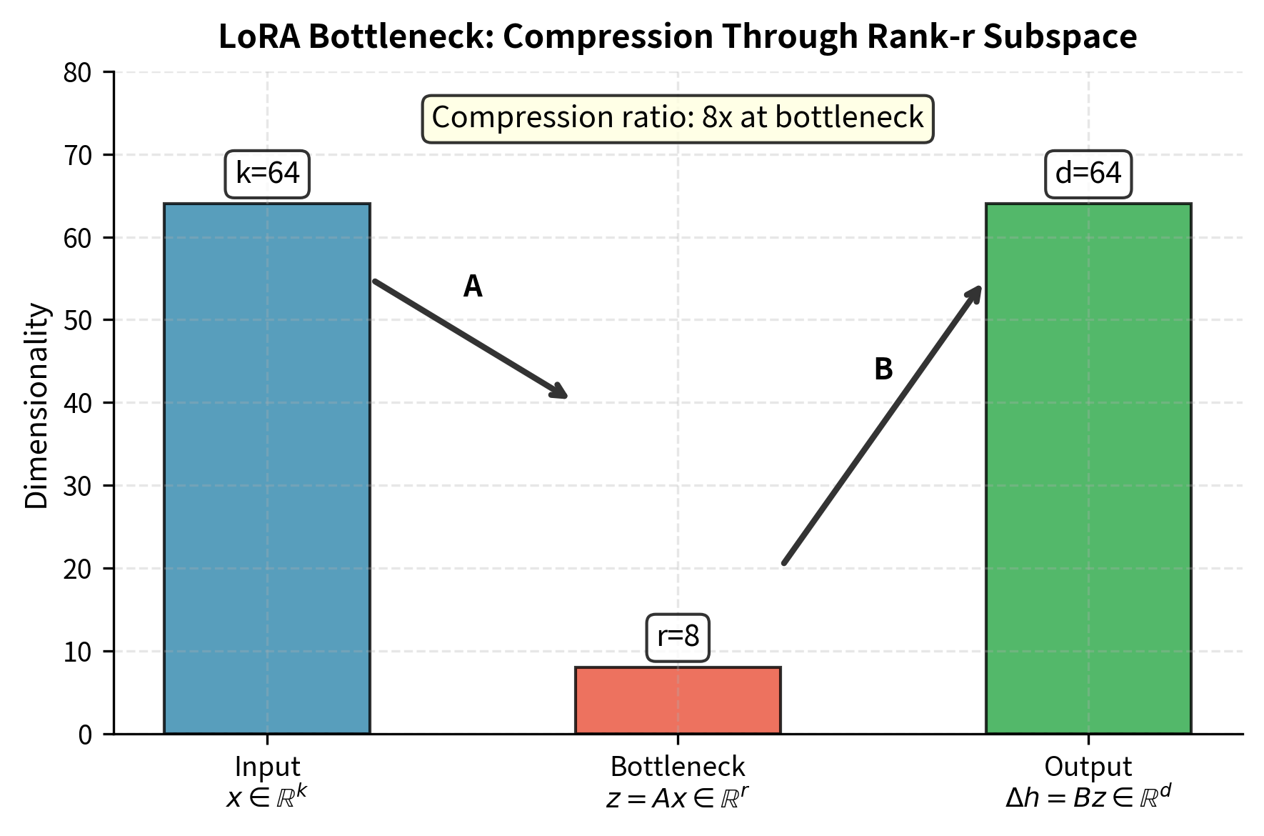
The rank constraint $\text{rank}(\Delta W) \leq r$ has a geometric interpretation that shows what LoRA learns during training. The matrix $\Delta W = BA$ maps inputs through an $r$-dimensional bottleneck, forcing all information about the input to pass through a low-dimensional representation before influencing the output.

Information flows through the LoRA path in three stages. First, the input vector $x$ is projected down to an $r$-dimensional representation $z$ by the matrix $A$. Then, this compressed representation is expanded back to the full output dimension by the matrix $B$. Mathematically:

where:

• $x$: the input vector
• $A$: the down-projection matrix
• $z$: the intermediate low-rank representation
• $B$: the up-projection matrix
• $\Delta h$: the update vector in the output space
• $r$: the rank of the adaptation
• $d$: the output dimension

This bottleneck structure implies several important properties. First, the update $\Delta h$ necessarily lies in the column space of $B$, which has dimension at most $r$. No matter what input $x$ we provide, the LoRA path can only produce outputs in this restricted subspace. Second, different inputs can only produce updates in this same $r$-dimensional subspace. The LoRA update cannot independently adjust every dimension of the output; it must work within the constraints of the learned subspace. Third, and importantly, the subspace is learned during training, not predetermined. The optimization process discovers which directions in weight space are most useful for the task at hand.

The training process simultaneously learns two complementary aspects of the adaptation. The matrix $B$ encodes which $r$-dimensional subspace in the output space should receive updates, effectively selecting the "directions" in which the model's behavior should change. The matrix $A$ encodes how to project inputs onto this subspace, determining which aspects of the input should influence these changes and by how much. Together, $A$ and $B$ learn both the structure of the adaptation and how to apply it based on the input.

Choosing the rank $r$ involves balancing expressiveness against efficiency. Rank is a primary hyperparameter in LoRA. Understanding its trade-offs is essential for practical application. Lower ranks use fewer parameters and computation but constrain the adaptation's capacity to represent complex changes to the model's behavior.

To understand the efficiency gains from LoRA, we need to compare the number of trainable parameters against full fine-tuning. For a weight matrix $W_0 \in \mathbb{R}^{d \times k}$, full fine-tuning requires learning $dk$ parameters. LoRA instead introduces:

where:

• $d$: output dimension of the layer
• $k$: input dimension of the layer
• $r$: rank of the adaptation

The parameter ratio compared to full fine-tuning reveals the compression achieved:

where:

• $dk$: total parameters in the full weight matrix
• $r(d+k)$: total parameters in the LoRA adapters
• $r$: rank of the adaptation
• $d$: output dimension
• $k$: input dimension

This ratio decreases as the layer dimensions grow, meaning LoRA becomes proportionally more efficient for larger models. For a transformer with $d = k = 4096$, which is typical of modern large language models, and $r = 16$:

where:

• $16$: the rank $r$ used in this example
• $4096$: the input and output dimensions ($d$ and $k$)
• $0.78\%$: the resulting parameter efficiency ratio

This calculation shows that LoRA with rank 16 uses less than 1 percent of the parameters that full fine-tuning would require for this single layer. The dramatic reduction holds across the entire model. If we apply LoRA to all attention projections (the query, key, value, and output matrices denoted $W_Q$, $W_K$, $W_V$, $W_O$) in each layer, the total trainable parameters remain a small fraction of the original model while still adapting the most important components of the transformer architecture.

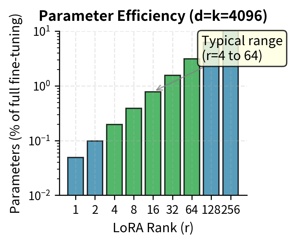
The rank determines the capacity of the adaptation, controlling how expressive the learned weight changes can be. Different ranks are appropriate for different scenarios:

• $r = 1$: The update is a rank-1 matrix $\Delta W = ba^T$ (outer product of two vectors). This is highly constrained, representing the simplest possible non-trivial update. Despite this severe limitation, rank-1 adaptations sometimes suffice for simple tasks like binary classification where the model primarily needs to adjust a single decision boundary.
• $r = 4$ to $r = 16$: These are common choices that balance efficiency and expressiveness for most NLP tasks. Many benchmarks show that ranks in this range achieve performance comparable to full fine-tuning while maintaining substantial parameter efficiency. This range represents the "sweet spot" for typical applications.
• $r = 64$ to $r = 256$: Higher capacity for complex adaptations, multi-task scenarios, or cases where lower ranks demonstrably underperform. These ranks sacrifice some efficiency for increased expressiveness, appropriate when the task demands more complex adaptations than lower ranks can represent.
• $r = \min(d, k)$: Full rank, equivalent to unconstrained fine-tuning of the layer. At this extreme, LoRA provides no parameter reduction but still maintains the structure of learning updates as a product of two matrices. This is primarily useful as a theoretical comparison point.

Empirically, rank selection depends on several factors that practitioners should consider. Task complexity plays a significant role. Simple classification may need only r = 8, while complex generation might benefit from r = 64 or higher. Dataset size interacts with rank in interesting ways. Smaller datasets benefit from lower ranks because the rank constraint provides implicit regularization, preventing overfitting. Larger datasets can exploit higher ranks without overfitting and may show continued improvement as rank increases. Finally, target modules often have different optimal ranks. Attention projections frequently need lower ranks than feed-forward layers, possibly because attention primarily routes information while feed-forward layers perform more complex transformations.

Trained LoRA adapters show an interesting pattern: even when $r$ is set relatively high, the effective rank of the learned $BA$ is often lower than the maximum possible. The optimization process tends to concentrate the adaptation into fewer dimensions than the allocated rank would allow.

The effective rank can be measured using the singular values of BA. One natural measure based on information theory follows.

where:

• $\tilde{\sigma}_i$: the normalized singular value such that $\sum \tilde{\sigma}_i = 1$
• $\sigma_i$: the $i$-th singular value of the matrix $BA$
• $\exp(\cdot)$: exponential function (computes the perplexity of the singular value distribution)

This entropy-based measure, sometimes called the spectral entropy or perplexity of the singular value distribution, indicates how many singular values contribute meaningfully to the matrix. If all $r$ singular values are equal, the effective rank equals $r$. If one singular value dominates, the effective rank approaches 1. Values between these extremes indicate intermediate concentration.

Studies examining trained LoRA adapters show that they often converge to solutions where only a few singular values dominate, even when the specified $r$ is much larger. This observation suggests that the actual intrinsic rank needed for the adaptation is lower than the specified $r$. It also suggests potential improvements: methods like AdaLoRA, covered in a later chapter, exploit this observation by adaptively adjusting the rank during training rather than fixing it in advance.

LoRA's initialization is crucial for training stability and convergence. How you initialize matrices $A$ and $B$ determines the model's starting point and influences the entire training trajectory. The standard scheme is:

• Matrix $A$: Initialized from $\mathcal{N}(0, \sigma^2)$ (Gaussian) or Kaiming initialization
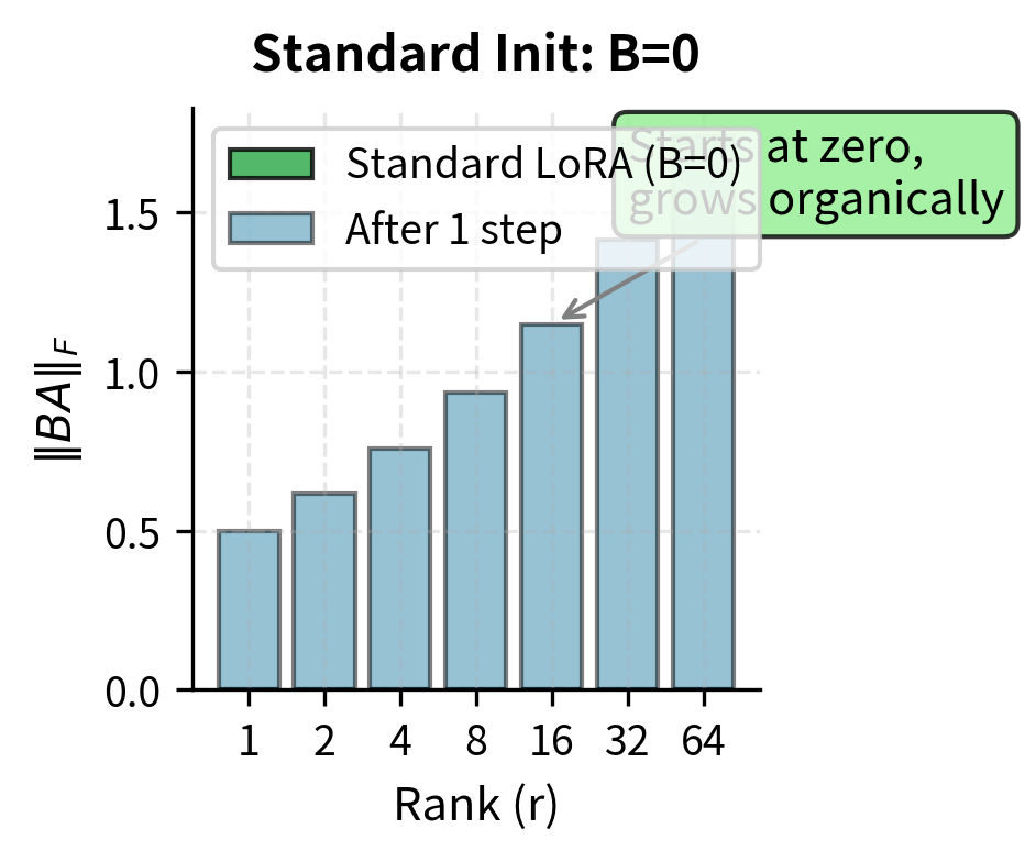
• Matrix $B$: Initialized to zero

This asymmetric initialization, with $A$ random and $B$ zero, ensures that the product $BA = 0$ at the start of training. This means the model begins with its pre-trained behavior completely intact: the LoRA path contributes nothing to the output until training begins to modify the parameters.

Starting with $\Delta W = BA = 0$ has several important advantages:

1. Continuity from pretraining: The model's initial behavior exactly matches the pretrained model. This is valuable because the pretrained model already performs well on many tasks. No "warm-up" period is needed for the model to recover from a random perturbation. From the first training step, we are refining good behavior rather than recovering from a disrupted starting point.

2. Stable training dynamics: Large random initializations of both $A$ and $B$ could produce $\|BA\|$ values that significantly perturb the pre-trained representations. If the initial perturbation is large, early training might focus on undoing this damage rather than learning the task. By starting at zero, we ensure that the first training steps are devoted entirely to task-relevant adaptation.

3. Gradient flow: A natural concern with zero initialization is whether gradients will flow properly. If $B = 0$ initially, won't the gradient with respect to $B$ also be zero, preventing any learning? Fortunately, this is not the case. The gradient with respect to $B$ depends on the input to the LoRA layer and the upstream gradient, not on the current value of $B$. As we'll derive in the gradient section below, $B$ receives non-zero gradients even when it equals zero.

The initialization variance explains why the standard scheme works better. If we initialize both $A$ and $B$ randomly with entries drawn from $\mathcal{N}(0, \sigma^2)$, what magnitude would we expect in the product $BA$?

For a single entry of the product:

where:

• $(BA)_{ij}$: element at row $i$, column $j$ of the product
• $B_{il}, A_{lj}$: elements of the random matrices
• $\sigma^2$: variance of the initialization distribution
• $r$: rank (number of terms in the sum)

The key observation is that this expected squared magnitude grows linearly with $r$. This rank dependence creates a problem: if we use the same initialization variance and learning rate for different ranks, higher ranks will produce larger initial perturbations and larger gradients. This would require rank-dependent learning rate adjustment to maintain consistent training dynamics. Zero-initializing $B$ sidesteps this issue entirely by ensuring the initial perturbation is exactly zero regardless of rank.

For matrix $A$, the standard initialization uses variance that scales inversely with rank:

where:

• $A_{lj}$: element of matrix $A$ at row $l$, column $j$
• $\mathcal{N}(\mu, \sigma^2)$: normal distribution with mean $\mu$ and variance $\sigma^2$
• $r$: rank of the adaptation
• $1/r$: variance chosen to scale with the rank

This scaling ensures that when gradients begin flowing and $B$ starts to move away from zero, the updates to $B$ have reasonable magnitude regardless of $r$. The variance is chosen so that the projection $Ax$ has expected squared norm that doesn't grow with $r$. Some implementations use Kaiming initialization instead, setting:

where:

• $A_{lj}$: element of matrix $A$
• $k$: input dimension of the layer

Kaiming initialization is designed to preserve the variance of activations through deep networks and is a reasonable alternative choice.

While zero-initialization of $B$ is standard and works well in most cases, researchers have explored alternatives that may offer advantages in certain scenarios:

• SVD initialization: Initialize $BA$ as a low-rank approximation of $W_{\text{fullfinetune}} - W_0$ from a reference full finetuning run. This requires running full fine-tuning once, but if you need to train many LoRA variants, initializing from the SVD of a reference solution can accelerate convergence significantly.
• Symmetric initialization: Initialize both $A$ and $B$ with small random values, accepting the initial perturbation to pre-trained behavior. This may help when the pre-trained model's initial behavior is far from desired, though it requires careful tuning of the initialization scale.
• Task-informed initialization: Use task-specific heuristics based on prior knowledge about the adaptation needed. For example, if adapting for a specific domain, initialize using SVD of domain-specific text representations.

We'll explore adaptive initialization strategies in the AdaLoRA chapter, where the initialization interacts with mechanisms that adjust rank during training.

Gradient flow through LoRA reveals training dynamics and connects to optimization concepts from Part VII. The gradient formulas reveal why the zero initialization of $B$ doesn't prevent learning and how $A$ and $B$ co-evolve during training.

Consider the forward pass for a single layer with LoRA adaptation:

where:

• $h$: the output vector
• $W_0$: the pre-trained weight matrix
• $x$: the input vector
• $\alpha$: the scaling factor
• $r$: the rank
• $B, A$: the LoRA up-projection and down-projection matrices

Let $\mathcal{L}$ be the loss function we're minimizing. To update $A$ and $B$ via gradient descent, we compute $\frac{\partial \mathcal{L}}{\partial A}$ and $\frac{\partial \mathcal{L}}{\partial B}$. The chain rule traces how parameter changes propagate through the computation to affect the loss.

First, let's define the upstream gradient. Let $\frac{\partial \mathcal{L}}{\partial h} = g \in \mathbb{R}^d$ be the gradient of the loss with respect to the layer's output. This gradient comes from the layers above in the network and tells us how changes in $h$ affect the loss.

For the gradient with respect to $B$, we apply the chain rule. The LoRA contribution to $h$ is $\frac{\alpha}{r} B(Ax)$. Differentiating this with respect to $B$, and then multiplying by how changes in $h$ affect the loss:

where:

• $\mathcal{L}$: the loss function
• $g$: the upstream gradient vector $\frac{\partial \mathcal{L}}{\partial h}$
• $Ax$: the intermediate vector (input projected down to rank $r$)
• $\alpha$: the scaling factor
• $r$: the rank

The gradient of $B$ is an outer product between the upstream gradient $g$ and the intermediate representation $Ax$. Each entry of the gradient $(B)_{il}$ measures how much increasing that entry would affect the loss, which depends on how much gradient signal arrives at output dimension $i$ (captured by $g_i$) and how active the corresponding bottleneck dimension $l$ was (captured by $(Ax)_l$).

For processing batches efficiently, we extend this to matrix form:

where:

• $\mathcal{L}$: loss function
• $\alpha$: scaling factor
• $r$: rank
• $G \in \mathbb{R}^{d \times n}$: matrix of upstream gradients for the batch
• $X \in \mathbb{R}^{k \times n}$: matrix of input vectors for the batch
• $A$: down-projection matrix

For the gradient with respect to $A$, we again apply the chain rule. Now we need to trace how changes in $A$ affect $h$ through the intermediate computation $Ax$:

where:

• $B^T$: transpose of the up-projection matrix
• $\mathcal{L}$: the loss function
• $\alpha$: the scaling factor
• $r$: the rank
• $g$: the upstream gradient vector
• $x$: the input vector

This formula shows that the gradient with respect to $A$ involves projecting the upstream gradient back through $B$ (using $B^T g$) and then forming an outer product with the input $x$. In matrix form for batch processing:

where:

• $\mathcal{L}$: loss function
• $\alpha$: scaling factor
• $r$: rank
• $B^T$: transpose of the up-projection matrix
• $G$: upstream gradient matrix
• $X^T$: transpose of the input batch matrix

Several properties of these gradients are noteworthy and reveal important aspects of LoRA's training dynamics.

Independence from $W_0$: The gradients $\frac{\partial \mathcal{L}}{\partial A}$ and $\frac{\partial \mathcal{L}}{\partial B}$ are independent of $W_0$. Frozen weights affect the upstream gradient $g$ but never appear explicitly in the LoRA gradient formulas. This separation enables efficient training where $W_0$ is never updated. You don't need to compute or store gradients for the much larger frozen weight matrices.

Coupled dynamics: Although $A$ and $B$ are separate parameters, their gradients are intimately coupled:

• $\frac{\partial \mathcal{L}}{\partial B}$ depends on $A$ through the term $Ax$
• $\frac{\partial \mathcal{L}}{\partial A}$ depends on $B$ through the term $B^T g$

This coupling means $A$ and $B$ co-evolve during training, with $A$'s current value determining $B$'s gradient and vice versa. This is similar to the dynamics in other factorized parameterizations, leading to interesting optimization behavior.

Zero initialization dynamics: At initialization ($B = 0$):

• $\frac{\partial \mathcal{L}}{\partial B} = \frac{\alpha}{r} g (Ax)^T \neq 0$ (generally non-zero)
• $\frac{\partial \mathcal{L}}{\partial A} = \frac{\alpha}{r} B^T g x^T = 0$

This asymmetry is important: $B$ updates immediately from the first gradient step, while $A$ has zero gradient initially. However, after the first update step, $B \neq 0$, and both matrices begin receiving non-zero gradients. The initial zero-gradient phase for $A$ is brief, lasting only a single step in theory, though in practice the gradients for $A$ remain small until $B$ has moved appreciably away from zero.

LoRA's gradient computations are efficient, requiring operations proportional to the parameter count rather than the full weight matrix size.

Computing $\frac{\partial \mathcal{L}}{\partial B} = \frac{\alpha}{r} g z^T$ where $z = Ax$ has the following costs: during the forward pass, we must store $z \in \mathbb{R}^r$, adding minimal memory overhead. The gradient computation itself is an outer product between vectors of dimension $d$ and $r$, requiring $O(dr)$ operations.

Computing $\frac{\partial \mathcal{L}}{\partial A} = \frac{\alpha}{r} B^T g x^T$ requires first computing $B^T g$, which is a matrix-vector product costing $O(dr)$ operations, followed by forming the outer product with $x^T$, which costs $O(rk)$ operations.

The total gradient computation is therefore $O(r(d + k))$, matching the parameter count. This is optimal. We need at least one operation per parameter to compute a gradient, and LoRA achieves this lower bound up to constant factors. This efficiency extends to the memory required for gradient storage, which also scales with $r(d+k)$ rather than $dk$.

Concrete numbers solidify the mathematical concepts. This example connects abstract formulas to actual numerical operations.

Consider a small weight matrix $W_0 \in \mathbb{R}^{4 \times 3}$ with rank r = 2 adaptation.

where:

• $W_0$: the pre-trained weight matrix

Initialize LoRA matrices following the standard scheme:

where:

• $A$: the down-projection matrix (randomly initialized)
• $B$: the up-projection matrix (initialized to zero)

For input $x = [1.0, 0.5, -0.2]^T$ with scaling factor $\alpha = 2$:

Forward pass:

Tracing through each step of forward computation:

1. Pre-trained output: We compute $W_0 x$ by multiplying the pre-trained weight matrix with the input. For the first element: $1.0 \cdot 1.0 + 0.5 \cdot 0.5 + (-0.3)(-0.2) = 1.0 + 0.25 + 0.06 = 1.31$. Continuing for all elements: $W_0 x = [1.31, 0.62, -0.15, 0.38]^T$

2. LoRA intermediate: We compute $z = Ax$, projecting the input down to the rank-2 bottleneck. First element: $0.3 \cdot 1.0 + (-0.5) \cdot 0.5 + 0.2 \cdot (-0.2) = 0.3 - 0.25 - 0.04 = 0.01$. Second element: $0.4 \cdot 1.0 + 0.1 \cdot 0.5 + (-0.3) \cdot (-0.2) = 0.4 + 0.05 + 0.06 = 0.51$. So $z = [0.01, 0.51]^T$

3. LoRA update: We compute $Bz$, projecting back up to the output dimension. Since $B = 0$, this gives $Bz = [0, 0, 0, 0]^T$

4. Final output: $h = W_0 x + \frac{\alpha}{r} Bz = [1.31, 0.62, -0.15, 0.38]^T + \frac{2}{2}[0, 0, 0, 0]^T = [1.31, 0.62, -0.15, 0.38]^T$

At initialization, the output equals the pre-trained output exactly. This confirms that zero-initializing $B$ preserves the pre-trained model's behavior.

Gradient computation:

With upstream gradient $g = [0.1, -0.2, 0.3, 0.1]^T$ from the loss and layers above, we compute gradients for both LoRA matrices.

For $B$:

where:

• $\mathcal{L}$: the loss function
• $B$: the up-projection matrix
• $\alpha$: the scaling factor ($\alpha = 2$)
• $r$: the rank ($r = 2$)
• $g$: the upstream gradient vector
• $z$: the intermediate activation vector computed in the forward pass

For $A$:

where:

• $\mathcal{L}$: the loss function
• $A$: the down-projection matrix
• $B^T$: the transpose of the up-projection matrix (currently zero)
• $g$: the upstream gradient vector
• $x$: the input vector

As expected from our theoretical analysis, $B$ receives non-zero gradients while $A$'s gradient is zero at initialization. After one gradient descent step updates $B$, subsequent forward passes will produce non-zero $B^T g$ terms, and $A$ will begin receiving gradients as well.

We'll implement the LoRA mathematics in PyTorch, demonstrating the forward pass, gradient computation, and initialization. The implementation verifies our theoretical predictions empirically.

Let's verify the initialization produces zero updates:

The product $BA$ is exactly zero because $B$ is initialized to zero, confirming our model starts with pretrained behavior. Matrix $A$ has dimensions (rank, in_features) for the down-projection, while $B$ has dimensions (out_features, rank) for the up-projection. Their product $BA$ maintains the full weight matrix dimensions but contains only zeros at initialization, meaning the LoRA path contributes nothing to the output until training begins.

Let's trace gradients through a forward-backward pass:

As predicted by analysis, matrix $A$'s gradient is zero at initialization because $B = 0$ in the gradient formula, while $B$ receives non-zero gradients. This asymmetry demonstrates the coupled dynamics derived mathematically. Matrix $A$ begins learning only after $B$ has moved away from zero, creating a brief initial phase where $B$ adapts alone before both matrices co-evolve.

Let's compute the parameter savings for a realistic scenario:

The 128x compression achieves dramatic parameter reduction while maintaining strong adaptation capability. Full finetuning of these attention layers requires 2.1 billion parameters, while LoRA needs only 16.8 million trainable parameters, making finetuning practical on consumer GPUs with 16-24GB of memory. This dramatic reduction enables efficient multi-task serving where different LoRA adapters can be swapped without duplicating the base model weights.

Let's visualize how different ranks affect the approximation capacity:

The error drops sharply until we reach the true intrinsic rank of the target matrix (8 in this case), then decreases more slowly. This shows why moderate ranks like 8 to 16 often suffice in practice.

Let's examine how gradients evolve during the first few training steps:

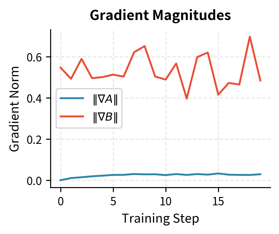
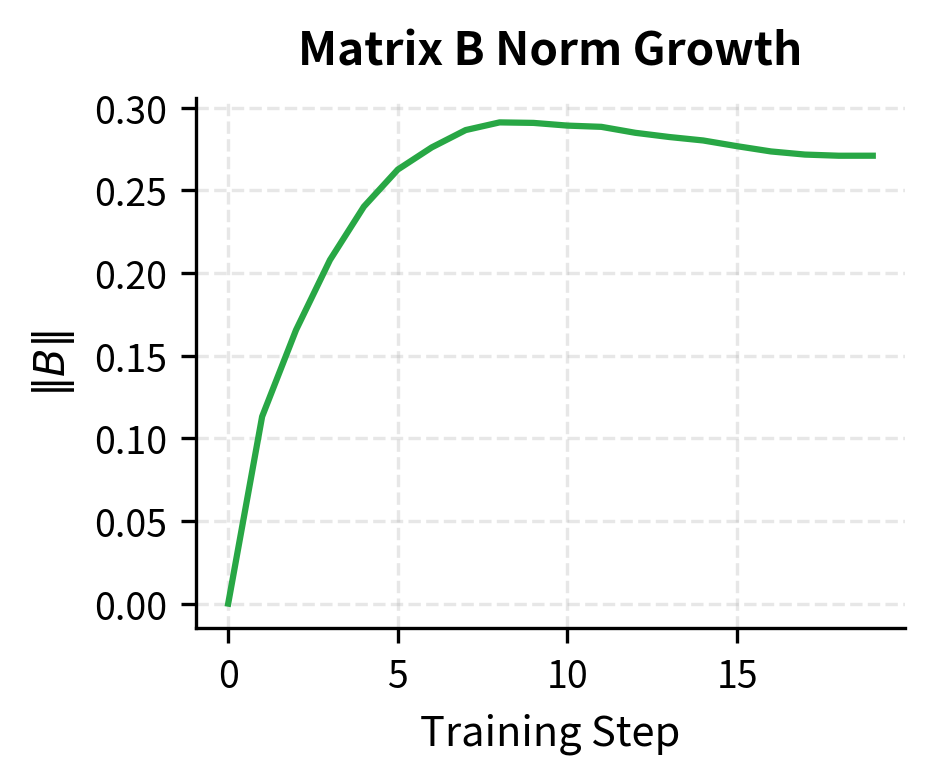
The plot confirms the mathematical analysis. Matrix A's gradient starts at zero and grows as B moves away from zero. The coupled dynamics quickly bring both matrices into active training.

LoRA's trained adapters can be merged into the base weights for inference: