LoRA Concept: Low-Rank Adaptation for Efficient LLM Fine-Tuning

The previous chapter established why parameter-efficient fine-tuning matters: full fine-tuning of large language models demands enormous memory, creates storage nightmares when serving multiple tasks, and risks catastrophic forgetting. But how do we actually reduce the number of trainable parameters without sacrificing model quality? Low-Rank Adaptation (LoRA), introduced by Hu et al. in 2021, provides an elegant answer rooted in a simple observation about how neural networks adapt to new tasks.

Weight updates during fine-tuning don't need the full capacity of the original weight matrices. When a 7-billion parameter model learns to follow instructions or answer questions in a specific domain, the changes to its weights occupy a much smaller "effective" space than the millions of parameters suggest. LoRA exploits this by representing weight updates as the product of two small matrices, dramatically reducing trainable parameters while preserving adaptation quality.

To understand LoRA, let's consider what happens inside a neural network during fine-tuning. Every pre-trained model begins its life through an extensive training process, learning patterns from massive datasets that might include books, websites, code repositories, and structured knowledge bases. This process produces a set of weight matrices that encode everything the model has learned: how to parse sentences, recognize named entities, reason about cause and effect, and generate coherent text. These weights represent the model's accumulated knowledge, frozen in numerical form.

When we fine-tune a pre-trained model, we start with weights $W_0$ learned during pre-training and update them based on our task-specific data. The fine-tuning process doesn't erase what the model already knows. Instead, it builds upon that foundation, adjusting the weights to emphasize patterns relevant to our particular task while preserving the general capabilities that make the model useful. Mathematically, the fine-tuning process results in a new set of weights expressed as the sum of the original weights and a task-specific update:

where:

• $W$: the final weights of the fine-tuned model (combining general and task-specific knowledge)
• $W_0$: the frozen pre-trained weights (which remain static to preserve prior knowledge)
• $\Delta W$: the accumulated weight update matrix (containing the learned adaptations)

This equation captures a fundamental truth about transfer learning: the fine-tuned model is the pre-trained model plus some modification. The modification, represented by $\Delta W$, encodes everything we want the model to learn from our task-specific data. If we're training a customer service chatbot, $\Delta W$ contains the adjustments that help the model use appropriate language, understand product-specific terminology, and respond to common customer queries. If we're building a medical assistant, $\Delta W$ encodes how to interpret clinical language and apply domain knowledge appropriately.

For a weight matrix in a transformer layer with dimensions $d \times k$, this update $\Delta W$ has exactly $d \times k$ parameters, the same as the original matrix. In standard fine-tuning, every element of the weight matrix can change, which requires tracking gradients, optimizer states, and values for millions of parameters.

In full fine-tuning, we compute gradients for every element of $W$ and update them all. As we discussed in the previous chapter on PEFT motivation, this approach becomes prohibitively expensive for modern LLMs. A single attention layer's query projection in a 7B parameter model might have dimensions like $4096 \times 4096$, meaning over 16 million parameters in just one weight matrix. When you consider that a typical transformer has dozens of layers, each containing multiple weight matrices for query, key, value, and output projections, plus feed-forward networks with their own massive weight matrices, the total parameter count quickly reaches into the billions.

Does $\Delta W$ need all those parameters to capture meaningful task adaptation? Consider what we're really doing when we fine-tune. We're not teaching the model to understand language from scratch. We're not rebuilding its world knowledge or its ability to reason. We're making relatively targeted adjustments, nudging the model to behave differently in specific ways relevant to our task. The update does not need full dimensionality.

LoRA is based on the idea that weight updates $\Delta W$ have low intrinsic rank. This means that even though $\Delta W$ is a large matrix, the information it contains can be compressed into a much smaller representation without significant loss. To understand this, we need to know what 'rank' is and why fine-tuning updates might have this property.

To understand what "low rank" means intuitively, consider what happens during fine-tuning. The pre-trained model has already learned rich representations of language: syntax, semantics, world knowledge, and reasoning patterns. These representations didn't emerge by accident. They developed through exposure to billions of tokens of text, refined through countless gradient updates that shaped the weight matrices into configurations that effectively model language. The resulting weights encode an incredibly sophisticated understanding of how words relate to each other, how concepts connect, and how reasoning unfolds.

When we fine-tune for a specific task like sentiment analysis or code generation, we're not fundamentally rebuilding these representations. Instead, we're making targeted adjustments: emphasizing certain features, suppressing others, and learning task-specific output patterns. A sentiment analysis fine-tuning might strengthen connections between emotional words and output decisions. A code generation fine-tuning might emphasize syntactic patterns relevant to programming languages. In both cases, we're working with what the model already knows, redirecting and refocusing rather than reconstructing.

These targeted adjustments don't require modifying every possible combination of input and output dimensions. Instead, they operate along a smaller number of "directions" in the weight space. Think of it like adjusting the equalizer on a stereo system: you have a few knobs that control broad frequency bands, not individual control over every single frequency. The adjustments you make are constrained to operate along a limited number of dimensions, yet they're sufficient to dramatically change the sound. Mathematically, this manifests as the update matrix having low rank.

Before looking at LoRA, we must understand matrix rank and why low-rank matrices are useful. Recall from our discussion of singular value decomposition in Part III that any matrix can be decomposed into a product of matrices revealing its underlying structure. This decomposition exposes the fundamental building blocks from which the matrix is constructed, much like factoring a number reveals its prime components.

The rank of a matrix tells us how many linearly independent rows or columns it contains, essentially measuring its "true" dimensionality. A matrix might appear large, with thousands of rows and columns, yet contain much less information than its size suggests. If many rows are simply linear combinations of other rows, or if many columns can be expressed as mixtures of other columns, the matrix has redundancy that can be exploited for compression.

A matrix with dimensions $d \times k$ can have rank at most $\min(d, k)$. If a matrix has rank $r$ much smaller than this maximum, it means the matrix contains redundant information that can be compressed. Specifically, a rank-$r$ matrix can be exactly represented as the product of two smaller matrices:

where:

• $M$: the target matrix to be approximated (of rank $r$)
• $B$: the first factor matrix with dimensions $d \times r$ (compressing information into $r$ columns)
• $A$: the second factor matrix with dimensions $r \times k$ (expanding information from $r$ rows)
• $r$: the rank of the decomposition (where $r \ll \min(d, k)$), controlling the compression ratio

This factorization is efficient. The total parameters in this factorized form are $dr + rk = r(d + k)$, which is much smaller than $dk$ when $r \ll \min(d, k)$. For example, if $d = k = 4096$ and $r = 8$, the original matrix requires $4096 \times 4096 = 16,777,216$ parameters, while the factorized form requires only $8 \times (4096 + 4096) = 65,536$ parameters. This represents a compression factor of 256, achieved without any loss of information if the original matrix truly has rank 8.

The factorized representation also has a clear geometric interpretation. Matrix $A$ projects inputs from the original $k$-dimensional space down to an $r$-dimensional bottleneck. Matrix $B$ then projects from this bottleneck back up to the $d$-dimensional output space. The bottleneck dimension $r$ controls how much information can flow through this narrow passage. When $r$ is small, only the most important patterns can survive the compression and expansion, effectively filtering out noise and redundancy.

Several factors support the low-rank assumption:

• Intrinsic dimensionality studies: Research shows that neural network learning trajectories often lie in low-dimensional subspaces. Even when training millions of parameters, the effective number of degrees of freedom is much smaller. Studies have measured the intrinsic dimensionality of various optimization problems and consistently found that successful solutions occupy a tiny fraction of the available parameter space. This suggests that gradient descent naturally finds solutions with low-dimensional structure.

• Empirical validation: The original LoRA paper showed that fine-tuning GPT-3 with rank as low as 4 or 8 matched full fine-tuning performance on many tasks. If the updates truly needed all $d \times k$ dimensions, such severe compression would destroy performance. Tiny adapters matching full fine-tuning performance shows that updates are approximately low-rank. Subsequent research has replicated these findings across models ranging from BERT to LLaMA, confirming the generality of this observation.

• Transfer learning intuition: Fine-tuning leverages pre-trained knowledge. We're not learning from scratch but nudging existing representations. This suggests the update should be "small" in some sense, and low rank is one way to formalize smallness. The pre-trained model already contains sophisticated representations; fine-tuning merely adjusts how those representations are combined and weighted for specific outputs. Such adjustments naturally involve fewer degrees of freedom than learning representations from scratch would require.

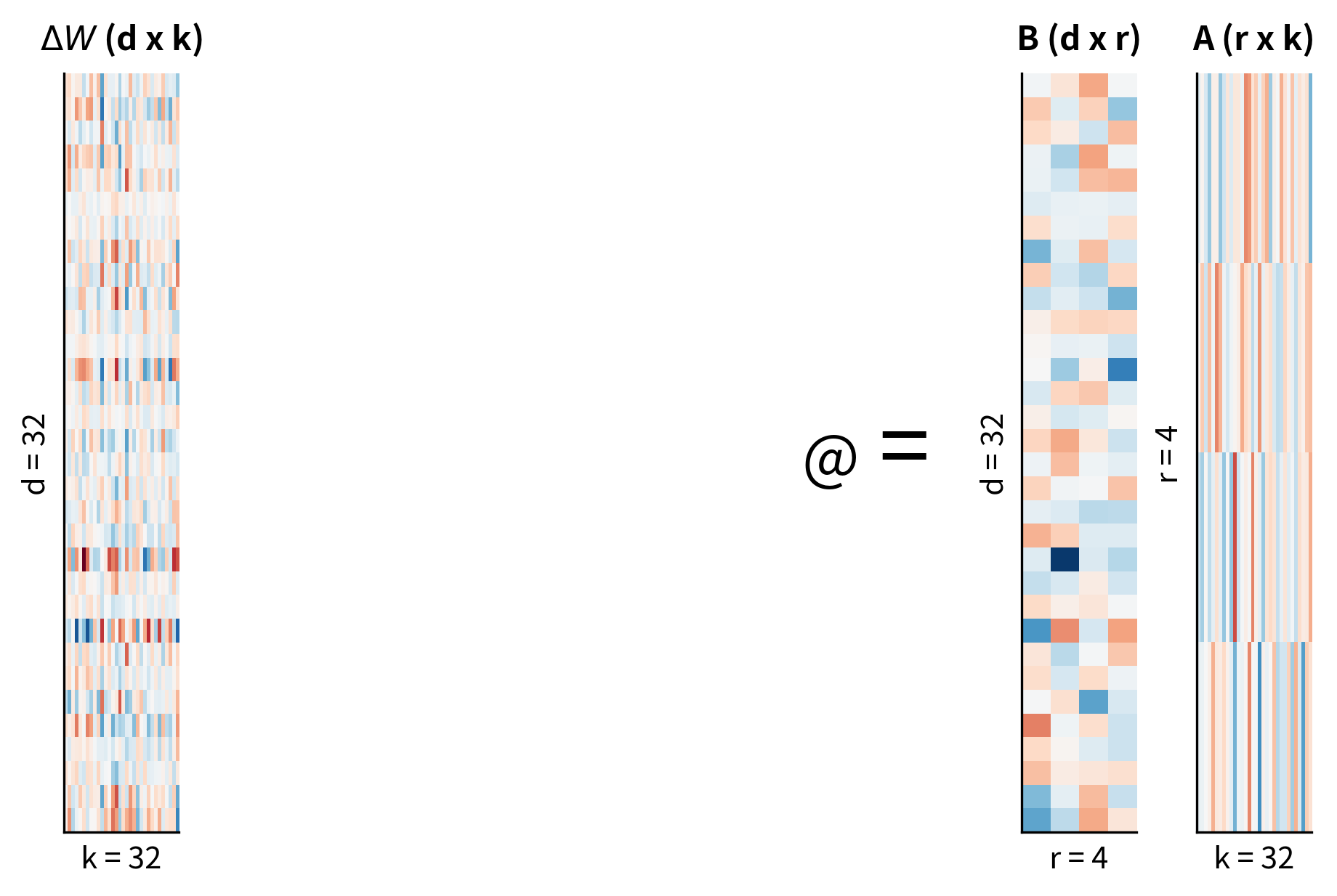
Given the low-rank assumption, LoRA's approach becomes clear: instead of learning the full update matrix $\Delta W$, learn its low-rank factors directly. This insight transforms the fine-tuning problem from learning millions of parameters to learning thousands, while preserving the model's ability to adapt effectively. We decompose the update into two smaller trainable matrices. LoRA constrains the update by defining it as the product of two low-rank matrices:

where:

• $\Delta W$: the accumulated weight update matrix (dimensions $d \times k$)
• $B$: the "up-projection" matrix ($d \times r$), which projects the low-rank signal back to the high-dimensional output space
• $A$: the "down-projection" matrix ($r \times k$), which projects the high-dimensional input to the low-rank bottleneck

The naming of these matrices reflects the information flow. When an input vector arrives at a layer, it first encounters matrix $A$, which compresses the $k$-dimensional input into an $r$-dimensional intermediate representation. This compression forces the adapter to identify the most task-relevant aspects of the input, discarding information that isn't useful for the current adaptation. Matrix $B$ then takes this compressed representation and expands it back to the $d$-dimensional output space, shaping how the compressed information influences the layer's output.

During the forward pass, the modified layer computes:

where:

• $h$: the output vector (containing features modified by the adapter)
• $W_0$: the frozen pre-trained weights (processing input using original knowledge)
• $\Delta W$: the accumulated weight update matrix
• $x$: the input vector (activation from the previous layer)
• $B$: the trainable up-projection adapter matrix
• $A$: the trainable down-projection adapter matrix

This formula shows LoRA's computation. Here, the term $W_0 x$ computes the features using the frozen pre-trained knowledge, exactly as the original model would. This keeps pre-trained capabilities active. The second term, $BA x$, computes the low-rank task-specific adjustment. This adjustment operates in parallel with the pre-trained computation, adding a correction signal that steers the output toward task-specific behavior.

The original pre-trained weights $W_0$ remain frozen throughout training; only the smaller matrices $B$ and $A$ receive gradient updates. This is the core mechanism that makes LoRA efficient. Because $W_0$ never changes, we don't need to store gradients for its millions of parameters. We don't need optimizer states like Adam's momentum and variance estimates for those parameters. The memory savings from freezing $W_0$ are enormous, and they stack multiplicatively: no gradients, no first moments, no second moments, no updated weight values to track.

With rank 8, we've reduced the trainable parameters by a factor of 256 compared to full fine-tuning of this layer. The original 16 million parameters become just 65,536 LoRA parameters. This dramatic reduction occurs because the low-rank factorization exploits the redundancy we hypothesize exists in fine-tuning updates. Rather than allowing arbitrary changes across all dimensions, we constrain changes to flow through a narrow bottleneck, capturing only the most essential adaptations.

The initialization of $B$ and $A$ affects training stability. A poor initialization might make the model erratic, causing outputs to diverge and destabilizing training. LoRA uses a specific initialization scheme designed to avoid these problems:

• $A$ is initialized from a Gaussian distribution (like typical weight initialization)
• $B$ is initialized to zero

Because B starts as a matrix of zeros, the product $BA$ is exactly zero regardless of what values $A$ contains. This means at the start of training, $\Delta W = BA = 0$, and the model behaves exactly like the pre-trained model. The first forward pass produces the same outputs the pre-trained model would produce. The first predictions are exactly what the base model would predict.

Training then gradually learns the task-specific update. As gradients flow backward through the network and update both $A$ and $B$, the product $BA$ slowly grows from zero, introducing task-specific modifications. The model's behavior shifts incrementally from pure pre-trained behavior toward task-adapted behavior. This initialization ensures we start from a known good state and make incremental modifications, never experiencing the instability that might arise from random, potentially harmful initial updates.

The zero initialization of $B$ guarantees that training starts from the exact pre-trained model behavior, ensuring stability in early training steps. This property is especially valuable when working with large models where instability can be difficult to diagnose and correct. By starting from a known good state, we can be confident that any changes in model behavior result from meaningful learning rather than initialization artifacts.

To build intuition for how well low-rank matrices can approximate full matrices, let's see how reconstruction error changes with rank. This visualization helps us understand why LoRA works: if typical weight updates have low intrinsic rank, then a low-rank representation should capture most of their information with minimal error. We'll create a synthetic example that mimics the structure of real weight updates, combining a low-rank signal with some noise.

The plot shows that once we reach the true intrinsic rank of the matrix, reconstruction error drops dramatically. Notice how the error curve has a sharp elbow around rank 16, which corresponds to the true rank of the underlying signal we constructed. Before this point, each additional rank dimension captures substantial information, leading to large reductions in error. After this point, additional dimensions primarily capture noise, yielding diminishing returns. For matrices with inherent low-rank structure, even aggressive compression preserves most information. This is exactly what LoRA exploits: if weight updates during fine-tuning are approximately low-rank, we can represent them efficiently without losing task performance. The key insight is that we don't need to know the true rank in advance. By choosing a rank that captures most of the error reduction, we can achieve excellent approximations with minimal parameter counts.

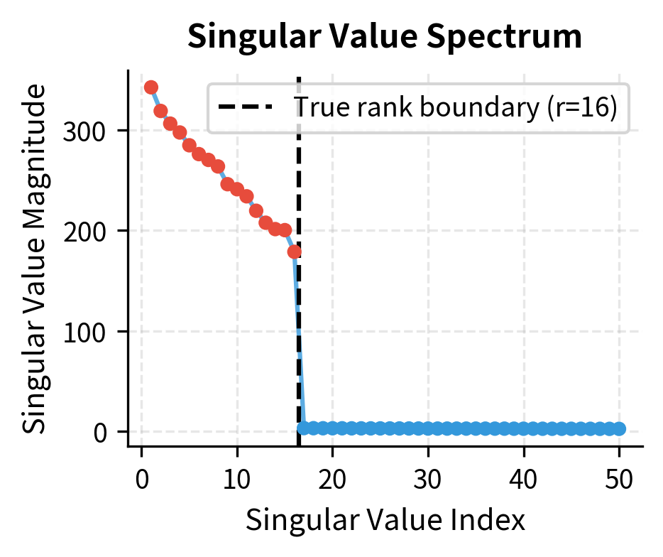
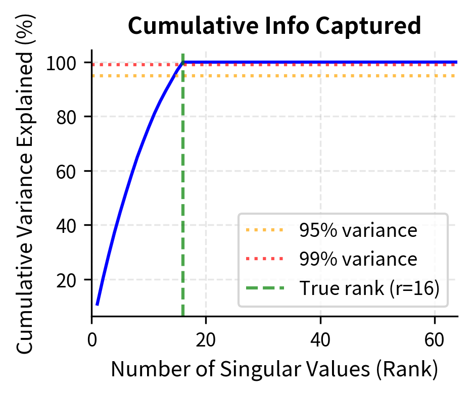
The singular value spectrum reveals why low-rank approximation works so well. The left panel shows that singular values drop sharply after the true rank of 16, meaning the remaining dimensions contribute little information. The right panel shows cumulative variance: a small number of dimensions capture nearly all the meaningful structure in the matrix. This pattern is exactly what we expect from fine-tuning updates, where task-specific modifications concentrate along a few important directions in weight space.

Reducing parameters through LoRA improves memory usage, training speed, and storage. These benefits compound across the training process and deployment lifecycle, making LoRA valuable not just for individual experiments but for entire ML workflows.

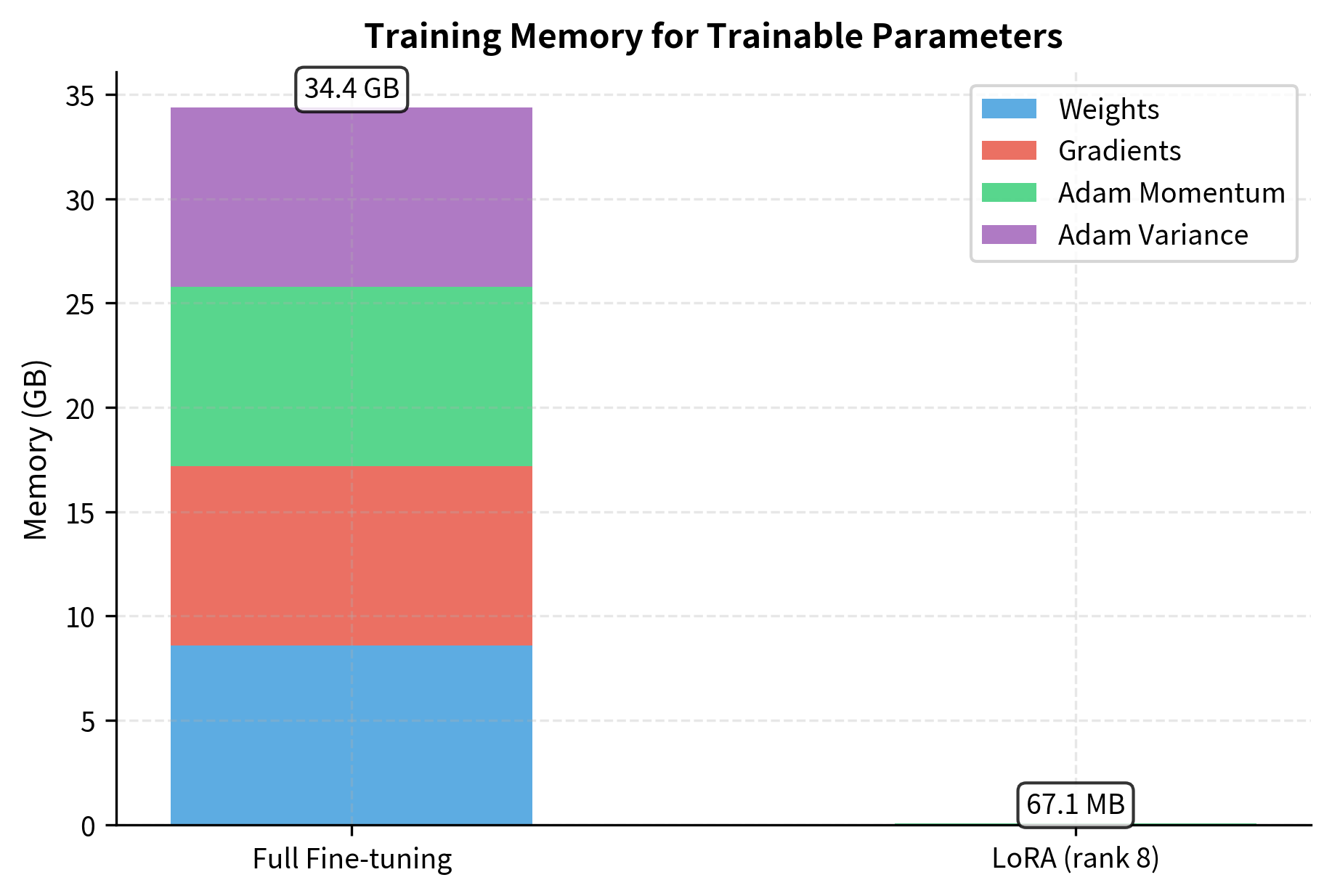
During training, memory consumption comes from several sources: model weights, gradients, optimizer states, and activations. Understanding each of these components helps explain why LoRA achieves such dramatic memory reductions. LoRA dramatically reduces the first three:

• Weights: The pre-trained weights $W_0$ stay frozen and don't need gradient computation. Only LoRA parameters ($A$ and $B$) are trainable. Because $W_0$ remains constant throughout training, we can store it in a memory-efficient format without worrying about tracking updates.

• Optimizer states: Adam maintains two additional tensors per parameter (first and second moment estimates), tripling memory for trainable parameters. With LoRA, these states only exist for the small adapter matrices. For a 7B parameter model, the optimizer states alone would require about 28GB for full fine-tuning, but LoRA reduces this to megabytes.

• Gradients: Only computed for LoRA parameters, not the full model. The backward pass still flows through the entire model to compute gradients for the adapter matrices, but we don't need to store or update gradients for the frozen weights.

This calculation only covers attention layers, but the pattern holds across the model. The memory savings enable fine-tuning on consumer GPUs that couldn't otherwise handle the full model. With a single RTX 3090, you can now fine-tune models that would otherwise require multiple A100 GPUs, democratizing access to state-of-the-art language model customization.

Fewer trainable parameters means less computation during the backward pass. While the forward pass remains similar (we still compute $W_0 x + BAx$), gradient computation only flows through the LoRA matrices. The optimizer step, which can be a significant portion of training time for large models, becomes much faster because it only updates thousands of parameters instead of billions.

In practice, training speedups are more modest than the parameter reduction suggests because:

1. The forward pass still involves the full pre-trained weights
2. Memory bandwidth often dominates over computation
3. Some overhead exists for managing the adapter structure

However, typical speedups of 1.5-3× over full fine-tuning are common, with larger gains when memory constraints force smaller batch sizes in full fine-tuning.

The most dramatic benefit is storage. With full fine-tuning, each task requires a complete copy of the model. For a 7B parameter model, that's approximately 14GB per task in fp16. Organizations deploying models for dozens or hundreds of different use cases would face storage costs that scale linearly with the number of tasks, quickly becoming prohibitive.

With LoRA, we store only the adapter weights. At rank 8 adapting 2 matrices per layer (typically query and value) across 32 layers, we might have around 4.2 million parameters, taking about 8MB in fp16. This represents a compression of over 1000×. The base model is stored once, and each task adds only a small adapter file.

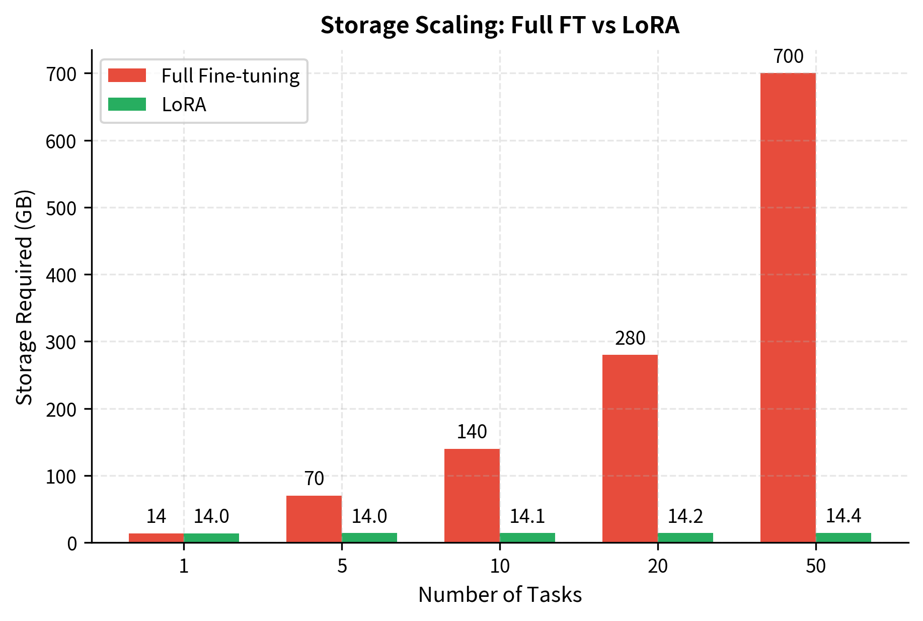
For serving 50 task-specific models, full fine-tuning requires 700GB of storage, while LoRA needs only about 14.4GB. This fundamentally changes the economics of deploying specialized models. Organizations can maintain extensive libraries of task-specific adapters, enabling personalization and specialization that would be impractical with full model copies.

Adapted weights can be merged back into the base model:

where:

• $W$: the merged weight matrix used for inference (functionally identical to a standard linear layer)
• $W_0$: the base model weights
• $B$: the learned up-projection adapter matrix
• $A$: the learned down-projection adapter matrix

The merge operation computes the matrix product $BA$ once, adds it to $W_0$, and stores the result. After merging, the model has exactly the same architecture as the original, with no additional computation during inference. The LoRA matrices disappear, leaving just a single weight matrix. This means that a LoRA-adapted model can achieve the exact same inference speed as the original pre-trained model, with no overhead from adapter computations.

This merge operation is optional. When you need to switch between tasks frequently, keeping adapters separate allows hot-swapping. When serving a single specialized model in production, merging eliminates any runtime overhead.

Beyond efficiency, LoRA provides flexibility in how and where adaptation is applied.

Not all weight matrices contribute equally to task adaptation. LoRA can be selectively applied to different components:\n\n- Attention projections: $W_Q$, $W_K$, $W_V$, $W_O$

• Feed-forward networks: Up and down projections, gate projections
• Embedding layers: Input and output embeddings

The original LoRA paper found that adapting query and value projections ($W_Q$ and $W_V$) provided most of the benefit, with diminishing returns from adding more matrices. We'll explore these hyperparameter choices in detail in an upcoming chapter.

This result highlights the extreme efficiency of LoRA. Making less than 1% of the parameters trainable significantly reduces the computational burden of gradient updates while maintaining the ability to adapt the model.

Since LoRA adapters are small and independent, a single base model can support many task-specific adapters simultaneously. This enables scenarios like:

• Multi-tenant serving: Different customers get personalized models from the same base
• A/B testing: Test different fine-tuning approaches with minimal overhead
• Composition: Combine adapters trained on different capabilities

The adapters can be swapped at runtime without reloading the base model, enabling flexible deployment architectures.

The rank $r$ provides a continuous trade-off between efficiency and expressiveness. Higher ranks allow capturing more complex adaptations but require more parameters. The relationship is straightforward: doubling the rank roughly doubles the number of adapter parameters, while potentially enabling the model to capture more nuanced task-specific adjustments. The optimal rank depends on:

• Task complexity: Simple classification might need rank 4; complex generation might benefit from rank 64
• Model size: Larger models may need higher ranks to maintain adaptation quality
• Dataset size: Limited data may favor lower ranks to prevent overfitting

We'll explore rank selection strategies in the hyperparameter chapter.

The visualization shows that LoRA parameters scale linearly with rank, providing a predictable trade-off between expressiveness and efficiency. Even at rank 64, which provides substantial adaptation capacity, LoRA uses less than 4% of the parameters that full fine-tuning would require. This linear scaling makes it easy to adjust the rank based on task requirements and available compute resources.

The key parameters for LoRA implementation are:

• rank ($r$): The dimensionality of the low-rank adapters. Lower ranks (4-8) are often sufficient for classification or simple tasks, while higher ranks (16-64) may be needed for complex reasoning or coding tasks.
• alpha: The scaling factor for the adapter output. A common heuristic is to set $\alpha = 2r$ or $\alpha = r$. It controls the magnitude of the update $\Delta W$ relative to the pre-trained weights.

Why does constraining updates to low rank work so well? The answer connects back to what pre-training accomplishes and reveals something fundamental about the nature of transfer learning.

Modern LLMs learn general-purpose representations during pre-training. They encode syntactic patterns, semantic relationships, factual knowledge, and reasoning heuristics. These representations exist in the high-dimensional space of the model's weights. Through billions of gradient updates on diverse text data, the model develops an incredibly rich internal language of features and transformations that can handle virtually any linguistic task.

Fine-tuning for a specific task doesn't require rebuilding these representations from scratch. Instead, it needs to:

1. Emphasize certain learned patterns relevant to the task
2. Suppress patterns that might interfere
3. Compose existing capabilities in task-specific ways
4. Learn a small amount of genuinely new task-specific information

All of these operations can be accomplished by adjustments along relatively few "directions" in weight space. Think of the pre-trained model as a powerful engine with many possible configurations. Fine-tuning doesn't rebuild the engine; it adjusts a few control settings to optimize for a specific use case. A low-rank update captures exactly this: targeted adjustments that leverage, rather than replace, pre-trained knowledge.

This perspective also explains why LoRA sometimes matches or exceeds full fine-tuning performance. By constraining updates to low rank, LoRA acts as a form of regularization, preventing overfitting to the fine-tuning dataset. The constraint forces the model to find solutions that work within the structure of pre-trained representations. If the fine-tuning dataset is small or noisy, this regularization effect can actually improve generalization compared to unconstrained full fine-tuning, which might memorize quirks of the training data rather than learning transferable patterns.

While LoRA offers substantial benefits, understanding its constraints helps you make informed decisions about when and how to apply it.

LoRA has some important limitations:

• Low-rank constraint may be suboptimal: Some tasks genuinely require updates that span many dimensions of weight space. In such cases, LoRA with small rank underperforms full fine-tuning. While increasing rank helps, very high ranks approach the parameter count of full fine-tuning, negating efficiency benefits.

• Additional hyperparameter complexity: Deciding which layers to adapt, selecting appropriate ranks, and tuning the scaling factor introduces hyperparameters that don't exist in standard fine-tuning. Suboptimal choices can hurt performance significantly.

• Linear combination assumption: The update $BA$ is simply added to $W_0$. More complex interactions between pre-trained and adapted weights aren't captured, potentially limiting expressiveness for some tasks.

• Dependence on pre-trained capabilities: LoRA works best when the base model already has relevant capabilities. If a task requires fundamental new knowledge not present in pre-training, no low-rank update can inject it. The technique excels at steering and specializing existing capabilities, not creating new ones from scratch.

LoRA's impact on the field has been substantial. It democratized fine-tuning by enabling adaptation of large models on consumer hardware. Researchers who couldn't afford multi-GPU clusters could suddenly fine-tune 7B or even 13B parameter models on a single GPU.

The technique also accelerated research by reducing experimental costs. When each fine-tuning run takes minutes instead of hours and requires gigabytes instead of terabytes, iteration speed increases dramatically. This has driven rapid progress in instruction tuning, alignment, and domain adaptation.

The multi-adapter paradigm enabled new deployment architectures. Services can maintain one base model and hundreds of customer-specific adapters, serving personalized experiences without the storage costs of full model copies.

LoRA also spawned a family of related techniques. As we'll see in upcoming chapters, variants like QLoRA (combining quantization with LoRA), AdaLoRA (adaptive rank allocation), and others build on LoRA's foundations to address specific limitations or use cases.

LoRA revolutionizes fine-tuning by recognizing that weight updates don't need full-rank expressiveness. The technique decomposes updates into two small matrices $B$ and $A$, dramatically reducing trainable parameters while maintaining adaptation quality.

The key concepts to remember:

• Weight decomposition: Instead of learning $\Delta W$ directly, LoRA learns $\Delta W = BA$ where $r \ll \min(d, k)$
• Low-rank assumption: Fine-tuning updates have low intrinsic dimensionality, making compression nearly lossless
• Zero initialization: $B$ starts at zero, ensuring training begins from exact pre-trained behavior
• Efficiency gains: 100-1000× fewer parameters translate to reduced memory, faster training, and compact storage
• Merge option: Adapters can be folded into base weights for zero-overhead inference
• Flexibility: Apply to selected layers, use multiple adapters, tune rank for task needs

The next chapter covers the math behind LoRA, including the forward and backward pass computations and its theoretical properties.

Ready to test your understanding? Take this quick quiz to reinforce what you've learned about Low-Rank Adaptation (LoRA) and its core concepts.