

A comprehensive guide to hypothesis testing in statistics, covering p-values, null and alternative hypotheses, z-tests for known variance and proportions, t-tests (one-sample, two-sample, paired, Welch's), F-tests for comparing variances and ANOVA for multiple groups, Type I and Type II errors, statistical power, effect sizes, and multiple comparison corrections. Learn how to make rigorous data-driven decisions under uncertainty.

This article is part of the free-to-read Machine Learning from Scratch
Choose your expertise level to adjust how many terms are explained. Beginners see more tooltips, experts see fewer to maintain reading flow. Hover over underlined terms for instant definitions.
Hypothesis Testing: Making Decisions Under Uncertainty
Hypothesis testing provides a rigorous framework for evaluating claims about populations using sample data. Rather than relying on intuition or subjective judgment, hypothesis testing establishes formal procedures for determining whether observed patterns in data reflect genuine phenomena or merely random chance. This framework underpins A/B testing in technology, clinical trials in medicine, quality control in manufacturing, and countless other applications where data-driven decisions matter.
Introduction
Every time you make a claim based on data, you face uncertainty. Did that new feature actually improve user engagement, or did you just happen to observe a lucky streak? Is the average response time of your system really above the acceptable threshold, or is the apparent problem just sampling noise? Hypothesis testing gives you a structured way to answer these questions, quantifying the strength of evidence and controlling the rate at which you make incorrect conclusions.
The core logic is surprisingly elegant. You start with a skeptical assumption, typically that nothing interesting is happening, and then ask: if this assumption were true, how surprising would my observed data be? If the data would be extremely unlikely under the skeptical assumption, you have grounds to reject it. If the data are reasonably consistent with the skeptical assumption, you lack sufficient evidence to claim otherwise.
This chapter builds from foundations to practical application. We begin with the precise definition of p-values, addressing common misconceptions that plague even experienced practitioners. We then establish the mechanics of hypothesis testing: formulating null and alternative hypotheses, choosing between one-sided and two-sided tests, and understanding critical regions and test statistics. The connection between hypothesis tests and confidence intervals reveals these as two sides of the same inferential coin.
We then examine the assumptions underlying common tests and what happens when they fail. The choice between z-tests and t-tests, between pooled and Welch's t-tests, depends on what you know about your data and what you can safely assume. Error analysis introduces Type I and Type II errors, leading naturally to the concept of statistical power and sample size determination. Finally, we address effect sizes, which tell you whether statistically significant results are practically meaningful, and multiple comparison corrections for when you conduct many tests simultaneously.
What a P-value Is (and Isn't)
The p-value is perhaps the most misunderstood concept in statistics. Before we can properly conduct or interpret hypothesis tests, we need a crystal-clear understanding of what p-values actually mean.
The p-value is the probability of observing data at least as extreme as the data actually observed, assuming the null hypothesis is true.
Let's unpack this definition carefully. The p-value is a conditional probability. It asks: given that the null hypothesis is true, what is the probability of seeing results as extreme as, or more extreme than, what we actually observed? The null hypothesis is the skeptical claim we are testing against, typically asserting no effect, no difference, or no relationship.
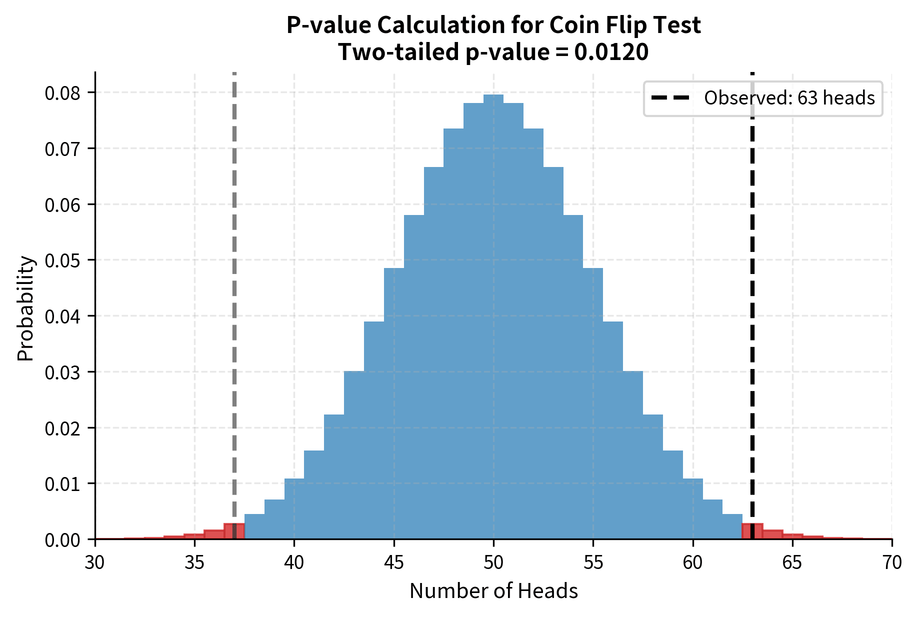
Consider a concrete example. Suppose you are testing whether a coin is fair. Your null hypothesis states that the probability of heads is 0.5. You flip the coin 100 times and observe 63 heads. The p-value answers the question: if the coin really were fair, what is the probability of getting 63 or more heads (or equivalently, 37 or fewer heads if we are doing a two-sided test)?
Common Misinterpretations
The p-value is emphatically not the probability that the null hypothesis is true. This is the single most common and consequential misinterpretation. The null hypothesis is either true or false; it is not a random variable with a probability distribution. The p-value tells you about the probability of the data given the hypothesis, not the probability of the hypothesis given the data.
Similarly, 1 minus the p-value is not the probability that the alternative hypothesis is true. A p-value of 0.02 does not mean there is a 98% chance that the effect is real. Converting p-values into statements about hypothesis probabilities requires Bayesian reasoning and prior probabilities, which classical hypothesis testing does not provide.
The p-value also does not measure the size or importance of an effect. A tiny, practically meaningless difference can produce a minuscule p-value if the sample size is large enough. Conversely, a substantial and important effect might yield a non-significant p-value if the sample is too small. The p-value speaks only to the evidence against the null hypothesis, not to the magnitude of any effect.
Why P < 0.05 Is Not a Magic Threshold
The conventional threshold of 0.05 for "statistical significance" is a historical convention, not a law of nature. Ronald Fisher originally suggested 0.05 as a reasonable threshold for preliminary evidence, but it has calcified into an arbitrary binary cutoff that distorts scientific practice.
A p-value of 0.049 is not fundamentally different from a p-value of 0.051. Both represent similar strength of evidence against the null hypothesis. Yet the former is often reported as "significant" and the latter as "not significant," leading to dramatically different conclusions and publication outcomes. This cliff-like treatment of a continuous quantity loses information and encourages practices like p-hacking, where researchers manipulate analyses until they achieve the magic threshold.
Better practice involves reporting exact p-values and interpreting them on a continuum. A p-value of 0.001 provides much stronger evidence against the null hypothesis than a p-value of 0.04, yet both clear the 0.05 threshold. Different contexts warrant different thresholds: particle physics famously uses 5-sigma (approximately p < 0.0000003) for discovery claims, while exploratory analyses might reasonably use p < 0.10. The appropriate threshold depends on the costs of different types of errors in your specific application.
Test Setup Basics
With the p-value concept firmly established, we can now examine the mechanics of setting up a hypothesis test. This involves formulating hypotheses, choosing the test type, and understanding how test statistics relate to sampling distributions.
Null vs Alternative Hypotheses
Every hypothesis test involves two competing hypotheses. The null hypothesis, denoted , represents the skeptical position, the claim we seek evidence against. Typically, the null hypothesis asserts that nothing interesting is happening: no difference between groups, no effect of a treatment, no relationship between variables. The null hypothesis is what we assume to be true unless the data provide sufficient evidence to the contrary.
The alternative hypothesis, denoted or , represents the research claim we seek to establish. It contradicts the null hypothesis and is what we accept if we reject the null. The alternative might claim that a treatment is effective, that two groups differ, or that a relationship exists.
For example, when testing whether a new drug lowers blood pressure:
- : The drug has no effect (mean blood pressure change = 0)
- : The drug lowers blood pressure (mean blood pressure change < 0)
Or when testing whether two teaching methods produce different outcomes:
- : The methods are equally effective (mean difference = 0)
- : The methods differ in effectiveness (mean difference 0)
The asymmetry between hypotheses is crucial. We never "accept" the null hypothesis; we either reject it or fail to reject it. Failing to reject is not the same as proving the null true. It simply means the data did not provide sufficient evidence against it.
One-Sided vs Two-Sided Tests
The choice between one-sided and two-sided tests depends on the research question and what alternatives are meaningful.
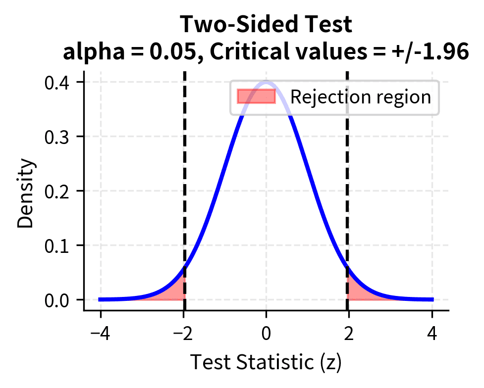
A two-sided test considers alternatives in both directions. When testing , the two-sided alternative is . You would reject the null if the sample mean is either much larger or much smaller than the hypothesized value. Two-sided tests are appropriate when departures from the null in either direction are scientifically meaningful and when you do not have strong prior reason to expect the effect to go in a particular direction.
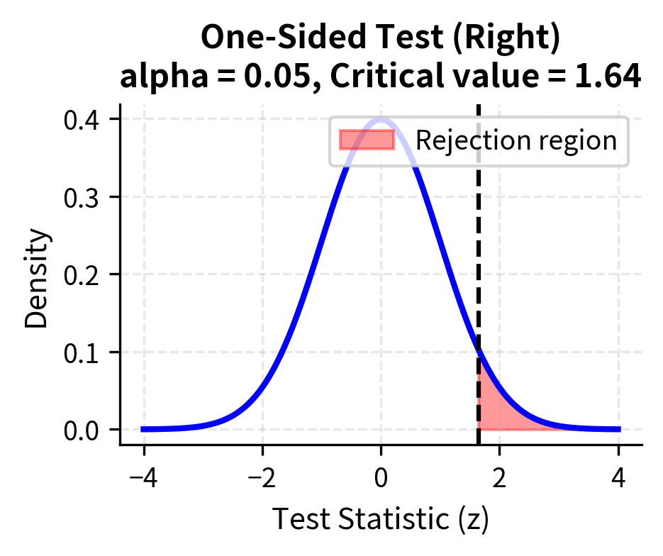
A one-sided test considers alternatives in only one direction. The alternative might be or . You specify before seeing the data which direction you expect, and you would only reject the null if the data deviate from the hypothesized value in that specific direction.
One-sided tests have more power to detect effects in the hypothesized direction because the entire significance level is concentrated in one tail. However, they cannot detect effects in the opposite direction, no matter how large. Using a one-sided test and then observing an effect in the unexpected direction creates an interpretive problem: technically, you should fail to reject the null, even if the effect in the "wrong" direction is substantial.
The choice should be made before examining the data, based on substantive considerations. If you would take the same action regardless of which direction an effect goes (for example, if any difference between methods warrants further investigation), use a two-sided test. If only one direction is scientifically meaningful or practically actionable (for example, you only care whether the new treatment is better, not whether it is worse), a one-sided test may be appropriate.
Test Statistics and Sampling Distributions
At the heart of every hypothesis test lies a simple but powerful idea: we need a single number that summarizes how strongly our data contradict the null hypothesis. This number is the test statistic, and understanding how to construct and interpret it is essential for mastering hypothesis testing.
A test statistic is a numerical summary of the data that captures how far the observed result deviates from what the null hypothesis predicts. But raw deviation alone is not enough. A sample mean that differs from the hypothesized value by 5 units might be highly significant or completely unremarkable, depending on how much variability we expect. If individual measurements typically vary by 2 units, a 5-unit difference is substantial. If they typically vary by 50 units, a 5-unit difference is noise.
This insight leads us to the most common form of test statistic, which measures deviation in standard error units:
This general formula captures the essence of hypothesis testing: measuring how far your observed result deviates from what the null hypothesis predicts, scaled by the uncertainty in your estimate. The numerator asks "how different is our observation from what the null hypothesis claims?" while the denominator asks "how much variation would we typically expect due to chance alone?" The ratio tells us how surprising our result is, expressed in standardized units that allow comparison across different contexts.
Think of it this way: if you observe a sample mean 2 standard errors away from the hypothesized value, you know your observation is moderately unusual under the null hypothesis, regardless of whether you're measuring heights in centimeters, weights in kilograms, or response times in milliseconds. This standardization is what makes hypothesis testing so broadly applicable.
Larger test statistics indicate observations that are less consistent with the null hypothesis. A test statistic of 0.5 suggests your observation is quite typical of what you'd expect if the null were true. A test statistic of 3 suggests your observation would be quite rare under the null hypothesis, providing strong evidence against it.
For testing a population mean, the z-statistic (when population standard deviation is known) or t-statistic (when it is unknown) takes this form:
where:
- : the sample mean, our best estimate of the population mean
- : the hypothesized population mean under
- : the known population standard deviation (for z-test)
- : the sample standard deviation (for t-test, used when is unknown)
- : the sample size
- or : the standard error of the mean
Let's trace through the logic of why each component is necessary. The numerator measures the raw discrepancy between what we observed and what the null hypothesis claims. If the null hypothesis states that the population mean is 100, and we observe a sample mean of 105, the numerator is 5. But as we noted, this raw difference is meaningless without context.
The denominator provides that context through the standard error. The standard error (or ) tells us how much sample means typically vary from sample to sample. If you drew many samples of size n from a population with mean and standard deviation , the sample means would cluster around with a standard deviation of . This is the standard error of the mean.
The critical insight is that the standard error shrinks as sample size grows, at a rate proportional to . With 4 times as many observations, the standard error is half as large. This reflects the fundamental statistical principle that averaging reduces noise: with more observations, random fluctuations tend to cancel out, and the sample mean becomes a more precise estimate of the population mean.
Under the null hypothesis, we know the probability distribution of the test statistic. This is the sampling distribution. It tells us what values of the test statistic we would expect to see if we repeated the sampling process many times and the null hypothesis were true. For the z-statistic, the sampling distribution is the standard normal distribution . For the t-statistic, it is a t-distribution with degrees of freedom. These distributions are completely specified, allowing us to compute exact probabilities.
The critical region consists of values of the test statistic that are sufficiently unlikely under the null hypothesis. If the calculated test statistic falls in the critical region, we reject the null hypothesis. The boundaries of the critical region are determined by the significance level . For a two-sided test at , the critical region includes values in both tails of the distribution, each tail containing 2.5% of the probability. For a one-sided test, all 5% is concentrated in one tail, making it easier to reject in the hypothesized direction but impossible to reject in the opposite direction.
The t-statistic of 0.502 indicates the sample mean is about half a standard error above the hypothesized mean of 100. The p-value of 0.6279 tells us that if the true mean were 100, we would observe a sample mean this far or farther from 100 about 63% of the time. This provides essentially no evidence against the null hypothesis.
Confidence Intervals as the Twin of Hypothesis Tests
Confidence intervals and hypothesis tests are mathematically equivalent tools that answer complementary questions. This equivalence is one of the most important conceptual insights in statistical inference, and understanding it deepens your appreciation of both methods.
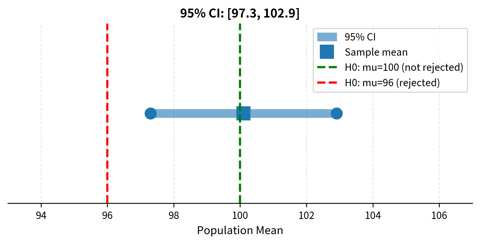
A 95% confidence interval contains all values of the parameter that would not be rejected by a two-sided hypothesis test at the 0.05 significance level. Conversely, a hypothesis test rejects the null hypothesis at level if and only if the hypothesized value falls outside the confidence interval. These are not just related tools. They are two perspectives on the same underlying calculation.
The CI-Hypothesis Test Equivalence
To see why this equivalence holds, consider how we construct each object. A 95% confidence interval for a population mean takes the form: for large samples with known variance (using critical values when variance is estimated). The interval extends 1.96 standard errors in each direction from the sample mean.
Now consider testing the null hypothesis at the 0.05 significance level. We reject when the z-statistic has absolute value exceeding 1.96. Rearranging this inequality:
This last condition is precisely the condition for to fall outside the confidence interval! If lies within 1.96 standard errors of , the hypothesis test fails to reject; if lies more than 1.96 standard errors away, the hypothesis test rejects. The confidence interval is the set of all values that would not be rejected.
This equivalence provides a powerful interpretation. A confidence interval shows you the range of parameter values that are "compatible" with your data at the specified confidence level. Any value inside the interval would not be rejected as a hypothesis; any value outside would be rejected. In this sense, the confidence interval is more informative than a single hypothesis test, telling you the result of infinitely many hypothesis tests at once.
For instance, suppose you calculate a 95% confidence interval of [2.3, 5.7] for the difference between two treatment means. This interval immediately tells you:
- would be rejected (0 is outside the interval)
- would not be rejected (3 is inside the interval)
- would be rejected (6 is outside the interval)
- Any value between 2.3 and 5.7 would not be rejected
Interpreting CI Width and Practical Meaning
The width of a confidence interval communicates the precision of your estimate. Narrow intervals indicate precise estimates; wide intervals indicate substantial uncertainty. Several factors affect interval width:
- Sample size: Larger samples produce narrower intervals because the standard error decreases as .
- Population variability: Greater variation in the population produces wider intervals.
- Confidence level: Higher confidence requires wider intervals to maintain coverage probability.
Beyond statistical significance, confidence intervals convey practical meaning. An interval of [0.1, 0.3] for an effect size suggests the effect is positive but small. An interval of [-0.5, 2.5] suggests substantial uncertainty about even the sign of the effect. This additional context is lost when you report only p-values or binary significance decisions.
Assumptions and What Breaks When They Fail
Every statistical test rests on assumptions about the data-generating process. When these assumptions are violated, the test may yield misleading results: p-values may be too small or too large, and Type I error rates may deviate from nominal levels. Understanding assumptions helps you choose appropriate tests and interpret results cautiously when assumptions are questionable.
Independence and Random Sampling
The most fundamental assumption for most tests is independence: observations should not influence each other. This assumption is violated in many practical situations:
- Repeated measures: Multiple observations from the same individual are correlated.
- Clustering: Students within the same classroom, patients at the same hospital, or observations from the same time period tend to be more similar than observations from different clusters.
- Time series: Sequential observations often exhibit autocorrelation.
Violating independence typically leads to underestimated standard errors and inflated Type I error rates. If you treat 100 observations from 10 people (10 per person) as if they were 100 independent observations, you dramatically overstate the effective sample size. The consequences can be severe: what appears to be strong evidence against the null hypothesis may simply reflect the dependence structure.
When independence is violated, use methods designed for the data structure: paired tests for matched data, mixed-effects models for clustered data, or time series methods for autocorrelated data.
Normality Assumptions
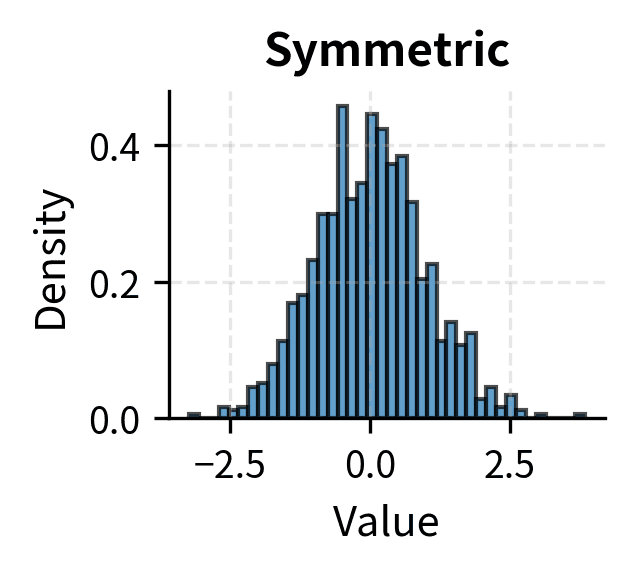
Many tests assume that the data, or certain functions of the data, are normally distributed. For t-tests and z-tests, the assumption is that the sampling distribution of the mean is normal. Thanks to the Central Limit Theorem, this is approximately true for large samples regardless of the population distribution, which is why these tests are often described as "robust to non-normality for large n."
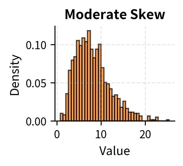
For small samples, the situation is more nuanced. Moderate departures from normality, such as mild skewness, typically have minor effects on t-test validity. Severe skewness, heavy tails, or outliers can substantially distort results, leading to either inflated or deflated Type I error rates depending on the specific departure.
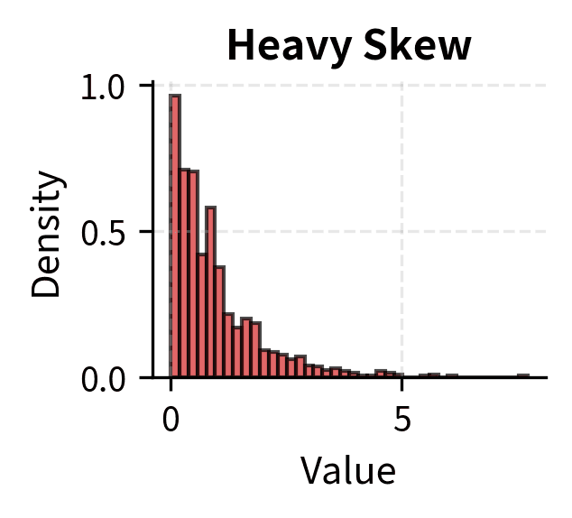
Rules of thumb suggest n > 30 is "large enough" for the CLT to provide adequate approximation, but this depends on how non-normal the population is. For heavily skewed distributions, even n = 100 may not be sufficient. When in doubt, use nonparametric tests that make fewer distributional assumptions, or use bootstrap methods to empirically assess the sampling distribution.
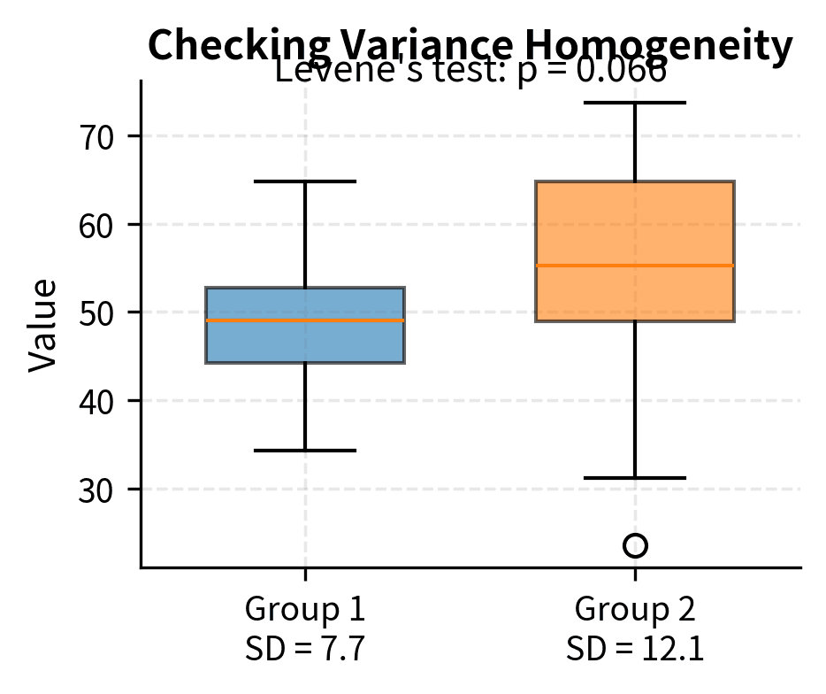
Equal Variances
Two-sample t-tests traditionally assume equal variances in the two populations (homoscedasticity). The pooled t-test uses this assumption to combine variance estimates from both groups, gaining precision when the assumption holds.
When variances differ substantially (heteroscedasticity), the pooled t-test can yield incorrect p-values. The Welch's t-test, which does not assume equal variances, is the safer default choice. It adjusts the degrees of freedom to account for unequal variances and performs nearly as well as the pooled test when variances are actually equal while providing valid inference when they are not.
When CLT Makes z/t "Okay Enough"
The Central Limit Theorem states that the sampling distribution of the mean approaches normality as sample size increases, regardless of the population distribution. This is the primary reason why t-tests and z-tests work so broadly: even when individual observations are non-normal, their averages tend toward normality.
The convergence rate depends on the population distribution. Symmetric distributions converge quickly; five or ten observations may suffice. Moderately skewed distributions require sample sizes of 30 to 50 for reasonable approximation. Heavily skewed or heavy-tailed distributions may require sample sizes in the hundreds.
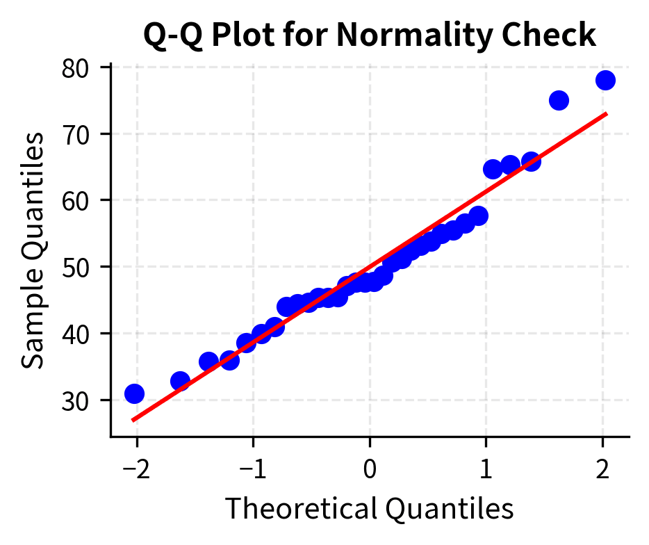
For practical purposes, if you have a sample size of at least 30, the t-test is usually acceptable unless you observe severe outliers or extreme skewness in your data. If you have smaller samples, check the data for obvious non-normality using histograms or Q-Q plots, and consider nonparametric alternatives if the assumption appears questionable.
Choosing Between z and t Tests
The choice between z-tests and t-tests hinges on whether the population standard deviation is known.
Known vs Unknown σ
The z-test assumes you know the population standard deviation . The test statistic is:
Under the null hypothesis, this follows a standard normal distribution exactly, regardless of sample size (assuming the population is normal) or approximately (for large samples from any distribution with finite variance).
In practice, knowing is rare. You might know it if the measurement process has been extensively calibrated, if you have very large historical data, or if external standards specify it. But in most research and data science applications, is unknown and must be estimated from the sample.
The t-test replaces with the sample standard deviation :
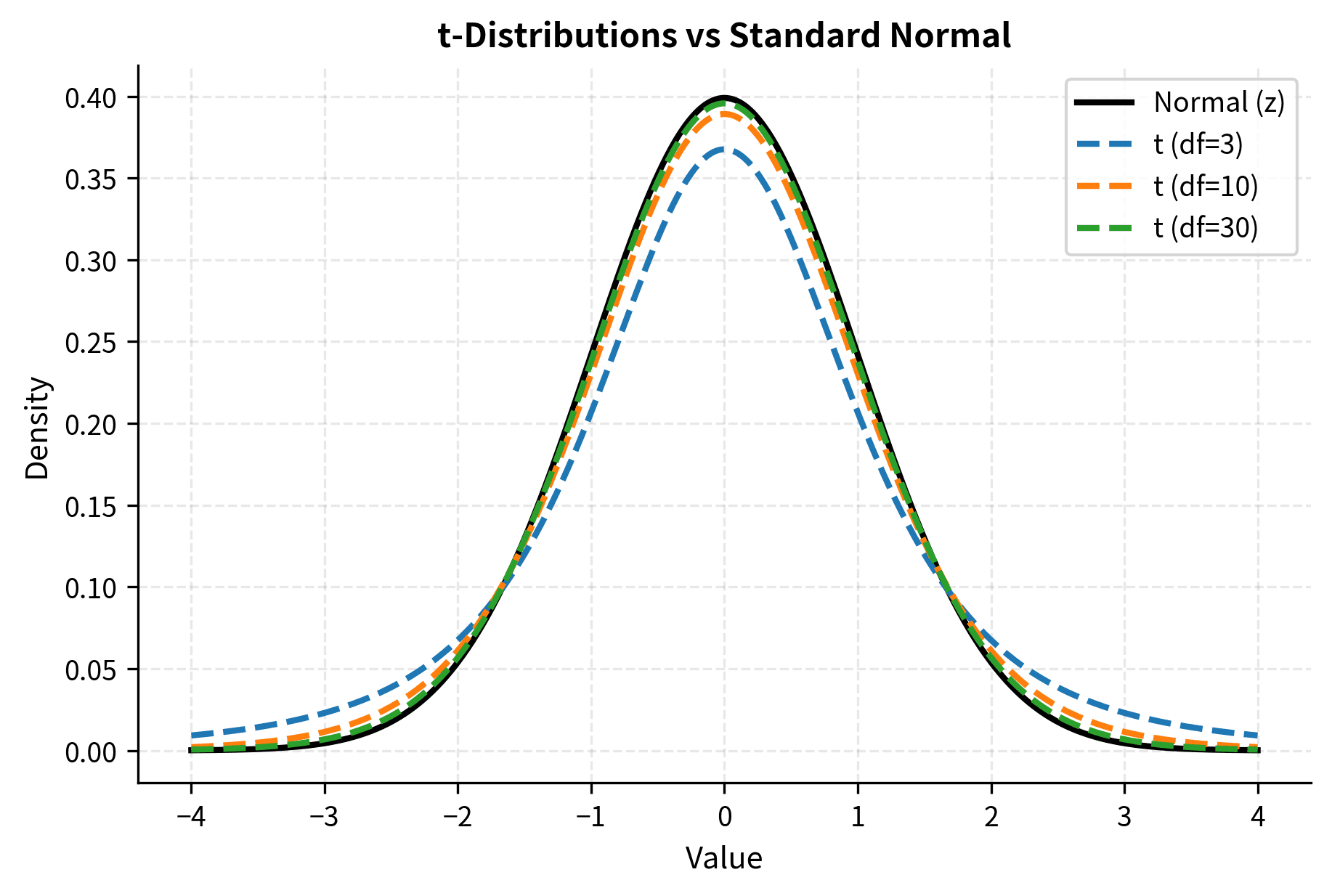
This substitution introduces additional uncertainty: itself is a random variable that varies from sample to sample. The t-distribution accounts for this extra uncertainty by having heavier tails than the normal distribution, yielding wider confidence intervals and larger p-values for the same observed deviation.
Small Sample Behavior
The t-distribution depends on the degrees of freedom, which for a one-sample test equals . With few degrees of freedom, the t-distribution is substantially heavier-tailed than the normal, and critical values are larger. As degrees of freedom increase, the t-distribution converges to the standard normal.
For sample sizes below 30, using the z-test instead of the t-test when is unknown can produce p-values that are too small, leading to inflated Type I error rates. Always use the t-test unless you have genuine prior knowledge of the population standard deviation.
Welch vs Pooled t-test
When comparing means between two independent groups, you have a choice between the pooled (Student's) t-test and Welch's t-test.
The pooled t-test assumes equal variances in both populations and combines (pools) the variance estimates:
where:
- : the pooled variance estimate, a weighted average of the two sample variances
- : the sample sizes of groups 1 and 2
- : the sample variances of groups 1 and 2
- and : degrees of freedom for each sample, which serve as weights
The weighting by degrees of freedom gives more influence to larger samples, which provide more reliable variance estimates. This pooled variance estimate is used to calculate the standard error of the difference in means.
Welch's t-test does not assume equal variances and uses a different formula for the standard error and degrees of freedom:
where:
- : the standard error of the difference between means
- : the sample variances of groups 1 and 2
- : the sample sizes of groups 1 and 2
This formula treats each group's variance independently, adding the variances of the two sampling distributions. The intuition is that the uncertainty in the difference comes from uncertainty in both means, and these uncertainties combine additively when the samples are independent.
The degrees of freedom are calculated using the Welch-Satterthwaite approximation, which is typically not an integer.
When variances are equal, both tests have similar power, though the pooled test is slightly more efficient. When variances differ, the pooled test can have either inflated or deflated Type I error rates depending on the relationship between variances and sample sizes. Welch's test maintains the correct Type I error rate regardless of variance equality.
Given this asymmetry, many statisticians recommend using Welch's test as the default for two-sample comparisons. You lose little when variances are equal and gain robustness when they are not.
In this example, both tests strongly reject the null hypothesis of equal means, but the test statistics and p-values differ slightly. When variances are dramatically different, the discrepancy can be much larger.
The Z-Test in Detail
The z-test is the simplest parametric test for comparing a sample mean to a hypothesized population mean. While rarely used in practice due to its requirement of knowing the population standard deviation, understanding the z-test provides essential foundation for grasping more complex tests. The z-test also applies directly in certain scenarios, particularly when working with proportions or when historical data provides reliable variance estimates.
When to Use the Z-Test
The z-test is appropriate under specific conditions:
- Known population standard deviation: You have reliable prior knowledge of from extensive historical data, calibration studies, or external standards.
- Large sample sizes: Even without knowing exactly, the z-test provides a reasonable approximation when n is very large (typically n > 100), because the t-distribution converges to the normal distribution.
- Testing proportions: When testing hypotheses about population proportions, the z-test is the standard approach, using the normal approximation to the binomial distribution.
In practice, genuine knowledge of is rare in research settings. You might encounter it in manufacturing contexts where measurement instruments have been extensively characterized, in standardized testing where population parameters are well-established, or when working with proportions where the variance is determined by the proportion itself.
Mathematical Foundation
To truly understand the z-test, we need to appreciate both the formula itself and the deep statistical reasoning that makes it work. The z-test rests on one of the most remarkable results in probability theory: when you know the population standard deviation, the sampling distribution of the mean follows a predictable pattern that we can exploit for inference.
The z-test statistic measures how many standard errors the sample mean lies from the hypothesized population mean:
where:
- : Sample mean, calculated as
- : Hypothesized population mean under
- : Known population standard deviation
- : Sample size
- : Standard error of the mean
Let's build intuition for why this formula works by tracing the logic step by step.
Step 1: The sampling distribution of the mean. When you draw a random sample of size n from a population with mean and standard deviation , the sample mean is itself a random variable. If you could repeat the sampling process infinitely many times, calculating a sample mean each time, those sample means would form a distribution called the sampling distribution of the mean. This distribution has two crucial properties:
- Its center (expected value) equals the population mean:
- Its spread (standard deviation) equals
The first property says that sample means are unbiased estimators of the population mean. On average, they hit the target. The second property says that sample means are more tightly clustered than individual observations, and the clustering improves with larger samples.
Step 2: Standardization. If we know and , we can standardize by subtracting its mean and dividing by its standard deviation:
This standardized variable Z has mean 0 and standard deviation 1. If the population is normally distributed, Z follows exactly a standard normal distribution . Even if the population is not normal, the Central Limit Theorem guarantees that Z will be approximately for large samples.
Step 3: Testing the hypothesis. Under the null hypothesis , we substitute for in the standardization formula:
If the null hypothesis is true, this z-statistic follows a standard normal distribution. We can therefore compute the probability of observing a z-statistic as extreme as (or more extreme than) the one we calculated. This probability is the p-value.
Under the null hypothesis, this z-statistic follows a standard normal distribution exactly when the population is normally distributed, and approximately when the sample size is large enough for the Central Limit Theorem to apply. This approximation is remarkably good even for moderately non-normal populations when n exceeds 30 or so.
The standard error deserves careful attention. It represents the standard deviation of the sampling distribution of the mean. While measures how much individual observations vary around the population mean, the standard error measures how much sample means would vary if you repeatedly drew samples of size n.
The factor of in the denominator reflects the reduction in variability achieved by averaging: with more observations, chance fluctuations tend to cancel out. This is sometimes called the "square root law" and has profound practical implications. To cut the standard error in half, you need to quadruple your sample size. To reduce it to one-tenth of its original value, you need 100 times as many observations. This diminishing return is why there is always a practical limit to how precise you can make your estimates through sheer sample size.
The beauty of the z-statistic is that it converts the complex question "Is my sample mean consistent with the null hypothesis?" into the simpler question "Is this number consistent with a standard normal distribution?" Since the standard normal distribution is completely characterized and tabulated, we can answer the second question precisely.
One-Sample Z-Test: Complete Procedure
Let's work through a complete one-sample z-test example. Suppose a manufacturer claims their light bulbs have a mean lifetime of 1000 hours, with a known population standard deviation of 100 hours (established through extensive quality testing). You sample 50 bulbs and find a mean lifetime of 975 hours. Is there evidence that the true mean differs from the claimed 1000 hours?
Step 1: State the hypotheses
- (The mean lifetime equals the claimed value)
- (The mean lifetime differs from the claimed value)
This is a two-sided test because we are interested in deviations in either direction.
Step 2: Choose the significance level
We use , accepting a 5% risk of false positive.
Step 3: Calculate the test statistic
Step 4: Determine the p-value or compare to critical values
For a two-sided test at , the critical values are . Since , the test statistic does not fall in the rejection region.
Alternatively, the p-value is .
Step 5: Make a decision
Since p = 0.0768 > 0.05, we fail to reject the null hypothesis. The sample does not provide sufficient evidence to conclude that the mean lifetime differs from 1000 hours.
The 95% confidence interval [947.28, 1002.72] contains the hypothesized value of 1000, which is consistent with failing to reject the null hypothesis. This illustrates the equivalence between confidence intervals and hypothesis tests.
Two-Sample Z-Test
When comparing means from two independent populations with known variances, the two-sample z-test is appropriate. The test statistic becomes:
Under the null hypothesis that (or more generally, that for some hypothesized difference ), this statistic follows a standard normal distribution.
The denominator is the standard error of the difference between means, calculated as the square root of the sum of the individual variances divided by their respective sample sizes. This formula assumes independence between the two samples.
Z-Test for Proportions
One of the most common applications of the z-test is testing hypotheses about population proportions. When the sample size is sufficiently large, the sample proportion is approximately normally distributed, enabling the use of z-test procedures.
For a one-sample test of a proportion, the null hypothesis specifies a value for the population proportion, and the test statistic is:
where:
- : the sample proportion (observed successes divided by sample size)
- : the hypothesized population proportion under
- : the sample size
- : the standard error of the proportion under the null hypothesis
Note that the standard error uses the hypothesized proportion rather than the sample proportion. This is because under the null hypothesis, we assume is the true proportion.
The normal approximation is generally considered adequate when both and . For smaller samples or proportions near 0 or 1, exact binomial tests or other methods may be more appropriate.
The T-Test in Detail
The t-test is the workhorse of hypothesis testing for means when the population standard deviation is unknown. Developed by William Sealy Gosset under the pseudonym "Student" in 1908 while working at the Guinness Brewery in Dublin, the t-test accounts for the additional uncertainty introduced by estimating the variance from the sample data. Gosset published under a pseudonym because Guinness had a policy against employees publishing scientific papers, fearing competitors might realize the advantage of employing statisticians.
The t-test solved a fundamental problem that had vexed statisticians. The z-test assumes we know the population standard deviation, but in practice we almost never do. When researchers simply substituted the sample standard deviation for the unknown population standard deviation and used normal distribution critical values, they made errors more often than they should have. Gosset showed that this substitution introduces additional variability that must be accounted for, and he derived the exact distribution of the resulting test statistic.
The Student's t-Distribution
When we replace the known population standard deviation with the sample standard deviation , the test statistic no longer follows a normal distribution. Instead, it follows a t-distribution with degrees of freedom determined by the sample size. Understanding why this happens deepens our appreciation of the t-test's elegance.
Consider what happens when we compute . The numerator and denominator are both random quantities that vary from sample to sample. In the z-test, the denominator is fixed at , so only the numerator varies. But in the t-test, we estimate the standard error from the same sample we use to compute the mean. This introduces a dependence between numerator and denominator that changes the distribution of the ratio.
The sample standard deviation is itself an imperfect estimate of . With small samples, can be considerably larger or smaller than by chance. When underestimates , the t-statistic is inflated, making our result appear more significant than it should. When overestimates , the t-statistic is deflated. On average, these errors don't favor either direction, but they do add variability to the test statistic.
The t-distribution captures exactly this additional variability. It has several key properties:
- Bell-shaped and symmetric about zero: Like the normal distribution, the t-distribution is unimodal and symmetric, centered at zero under the null hypothesis.
- Parameterized by degrees of freedom (df): The shape depends on df, which typically equals for a one-sample test. The degrees of freedom represent the amount of independent information available to estimate the variance. With more degrees of freedom, we have a better estimate of , and the t-distribution becomes closer to normal.
- Heavier tails than normal: The t-distribution has more probability in its tails than the standard normal. This means extreme values are more likely, reflecting the uncertainty added by estimating the variance.
- Converges to normal: As df increases, the t-distribution approaches the standard normal distribution. For df > 30, the two are nearly identical, which is why older textbooks sometimes say "use z for large samples." For df > 100, the difference is negligible for practical purposes.
- Accounts for estimation uncertainty: The heavier tails appropriately penalize us for not knowing the true population variance. This penalty is larger for smaller samples, where our variance estimate is less reliable.
The heavier tails of the t-distribution mean that extreme values are more probable than under the normal distribution. This translates to larger critical values and wider confidence intervals, appropriately penalizing us for not knowing the true population variance. For example, with 5 degrees of freedom, the two-sided critical value at is 2.571, substantially larger than the normal value of 1.96. With 30 degrees of freedom, it drops to 2.042, quite close to 1.96.
The mathematical derivation of the t-distribution involves the ratio of a standard normal random variable to the square root of an independent chi-squared random variable divided by its degrees of freedom. While this may sound esoteric, the practical consequence is simple: use t-distribution critical values when you estimate variance from the sample, and use normal critical values only when you genuinely know the population variance or have a sample so large that the distinction is irrelevant.
One-Sample T-Test: Complete Procedure
The one-sample t-test compares a sample mean to a hypothesized population mean when the population variance is unknown. The test statistic is:
This follows a t-distribution with degrees of freedom under the null hypothesis.
Let's work through a detailed example. A coffee shop claims their large drinks contain 16 ounces. You measure 15 randomly selected drinks and find a mean of 15.6 ounces with a sample standard deviation of 0.8 ounces. Is there evidence that the true mean differs from the claimed 16 ounces?
The sample mean of 15.66 ounces is below the claimed 16 ounces, and with p = 0.0418 < 0.05, we reject the null hypothesis. The 95% confidence interval [15.35, 15.97] does not contain 16, consistent with our rejection. Note how the confidence interval and hypothesis test give the same conclusion, as they must mathematically.
Independent Two-Sample T-Test
The two-sample t-test compares means from two independent groups. There are two variants: the pooled (Student's) t-test assuming equal variances, and Welch's t-test which does not assume equal variances.
Pooled T-Test (Equal Variances)
When population variances are assumed equal, we pool the sample variances to get a more precise estimate. The pooled variance is:
where:
- : the pooled variance estimate
- : sample sizes for groups 1 and 2
- : sample variances for groups 1 and 2
- : total degrees of freedom (each group contributes )
This is a weighted average of the sample variances, with weights proportional to degrees of freedom. The test statistic is:
where:
- : the observed difference in sample means
- : the pooled standard deviation (square root of pooled variance)
- : a factor that accounts for the sample sizes in both groups
The denominator is the standard error of the difference between means. This follows a t-distribution with under the null hypothesis.
Welch's T-Test (Unequal Variances)
When we cannot assume equal variances, Welch's t-test uses a different standard error:
The degrees of freedom are calculated using the Welch-Satterthwaite approximation:
where:
- : the effective degrees of freedom for the t-distribution
- : sample variances for groups 1 and 2
- : sample sizes for groups 1 and 2
This formula estimates how many degrees of freedom the combined variance estimate effectively has. When variances are unequal, the effective degrees of freedom is reduced, making the test more conservative (wider confidence intervals, larger p-values). This complex formula typically yields a non-integer degrees of freedom, which is handled by interpolation or by rounding down for a more conservative test.
Both tests yield highly significant results (p < 0.001), with Method B showing substantially higher scores. Cohen's d of 2.41 indicates a very large effect size. The similarity between pooled and Welch's results here reflects that the sample variances are similar; when variances differ more substantially, the tests would diverge.
Paired T-Test
The paired t-test is used when observations come in matched pairs, such as before-after measurements on the same subjects, or matched case-control studies. By analyzing the differences within pairs, the paired t-test controls for individual variation, often resulting in more powerful tests than independent two-sample comparisons.
The test statistic is simply a one-sample t-test on the differences:
where:
- : the mean of the paired differences (after minus before, or treatment minus control)
- : the standard deviation of the differences
- : the number of pairs
- : the standard error of the mean difference
This follows a t-distribution with degrees of freedom. The key insight is that by computing differences within pairs first, we reduce the problem to a one-sample test, eliminating between-subject variability that would otherwise obscure the treatment effect.
The paired t-test reveals a significant reduction in blood pressure (mean decrease of 6.3 mmHg, p < 0.001). The confidence interval [-8.56, -4.04] excludes zero, confirming the significant effect. The paired design is powerful here because it eliminates between-subject variability, focusing only on within-subject changes.
Assumptions of T-Tests and Checking Them
T-tests rely on several assumptions. Violating these assumptions can affect the validity of conclusions:
-
Independence: Observations should be independent (or, for paired tests, the pairs should be independent of each other).
-
Normality: The sampling distribution of the mean should be approximately normal. This is satisfied when:
- The population is normally distributed, OR
- The sample size is large enough for the CLT to apply (typically n > 30)
-
Homogeneity of variance (for pooled two-sample t-test only): The population variances should be equal.
Here's how to check these assumptions:
Deciding Which Test to Use: A Decision Framework
Choosing the right t-test variant depends on your research design and data characteristics:
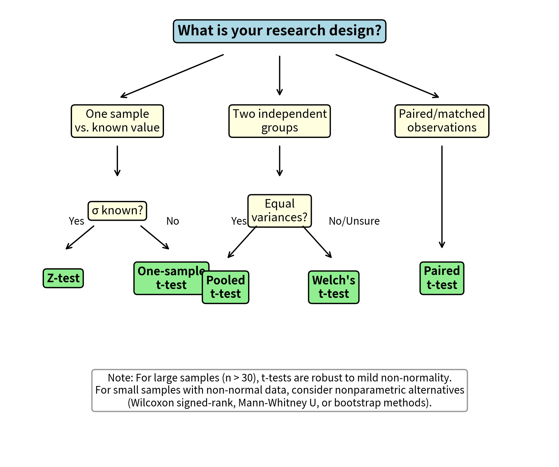
The key recommendations are:
- One sample, σ known: Use z-test (rare in practice)
- One sample, σ unknown: Use one-sample t-test
- Two independent samples, equal variances: Pooled t-test or Welch's t-test
- Two independent samples, unequal variances: Welch's t-test
- Two independent samples, uncertain about variances: Default to Welch's t-test
- Paired/matched observations: Paired t-test
When in doubt between pooled and Welch's t-tests, choose Welch's. You sacrifice minimal power when variances are equal but gain robustness when they are not.
The F-Test and F-Distribution
While z-tests and t-tests focus on comparing means, the F-test addresses a different but equally important question: comparing variances. The F-test also forms the foundation for Analysis of Variance (ANOVA), which extends hypothesis testing to compare means across three or more groups. Understanding the F-distribution and its applications is essential for regression analysis, experimental design, and many advanced statistical methods.
The F-test is named after Sir Ronald A. Fisher, one of the founders of modern statistics, who developed much of the theory of variance analysis in the 1920s. Fisher recognized that many important questions in science and industry involve comparing sources of variation rather than just means. Is one manufacturing process more variable than another? Do different treatments produce different amounts of variation in patient outcomes? Does adding predictors to a regression model significantly reduce residual variance? These questions all lead naturally to F-tests.
The F-Distribution
To understand the F-test, we must first understand where the F-distribution comes from and why it arises when comparing variances.
Recall that when we estimate variance from a sample, we compute . If the underlying population is normally distributed with variance , then the quantity follows a chi-squared distribution with degrees of freedom. This is because it is a sum of independent squared standard normal random variables (the comes from losing one degree of freedom when we estimate the mean).
Now suppose we have two independent samples, each from a potentially different population. From the first sample, we compute , and from the second, . If both populations are normal with the same variance , then:
The F-distribution arises naturally when comparing two independent estimates of variance. If you have two independent chi-squared random variables divided by their respective degrees of freedom, their ratio follows an F-distribution:
where:
- : the F-statistic, a ratio of variance estimates
- : chi-squared distributed random variables (sums of squared normal deviates)
- : degrees of freedom for the numerator and denominator, typically and
- : sample variances from two populations
- : true population variances
When (the null hypothesis of equal variances), the ratio simplifies beautifully. The unknown common variance cancels from numerator and denominator, leaving:
This ratio of sample variances, under the null hypothesis, follows an F-distribution with and degrees of freedom. The beauty of this result is that we can test whether two population variances are equal without knowing what those variances actually are.
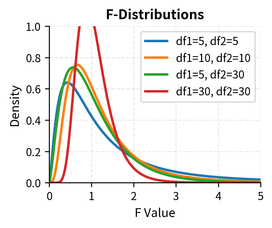
The F-distribution has several distinctive properties that set it apart from the normal and t-distributions:
- Two degrees of freedom parameters: Unlike the t-distribution with one df parameter, the F-distribution requires two: (numerator) and (denominator). The order matters! is different from .
- Always non-negative: Since it is a ratio of squared quantities (variances are always positive), F is always greater than or equal to zero. There are no negative F-values.
- Right-skewed: The distribution is asymmetric, with a long right tail. As both df increase, it becomes more symmetric and concentrated, approaching normality.
- Mean approximately 1 under the null: When the null hypothesis is true (equal variances), the expected value of F is close to 1, specifically for . This makes intuitive sense: if two variances are equal, their ratio should be around 1.
F-Test for Comparing Two Variances
The simplest application of the F-test compares variances between two independent populations. While less famous than its cousin for comparing means, this test addresses practical questions that arise frequently in applied work:
- Checking the equal variance assumption: Before using a pooled t-test, you need to verify that the two populations have similar variances. The F-test provides a formal way to check this assumption.
- Comparing process variability: In manufacturing and quality control, consistency often matters as much as the average. Two production lines might produce the same average output, but one might be more variable, leading to more defects.
- Risk assessment: In finance, comparing the variances of two investments tells you about their relative risk, even if their expected returns are similar.
- Method comparison: When evaluating two measurement methods, you might want to know if one produces more variable results than the other.
The logic of the F-test for variances is elegantly simple. If two populations have the same variance, then sample variances drawn from those populations should be similar to each other. Their ratio should be close to 1. If the ratio is far from 1, we have evidence that the population variances differ.
The test statistic is the ratio of the two sample variances:
where:
- : the F-statistic for comparing variances
- : sample variance of the first group (typically placed as the larger variance)
- : sample variance of the second group
Let's trace through why this ratio works. Each sample variance estimates its corresponding population variance . If the null hypothesis is true, both sample variances are estimating the same quantity. The ratio should therefore fluctuate around 1, with the fluctuation determined by the sampling distribution of the ratio.
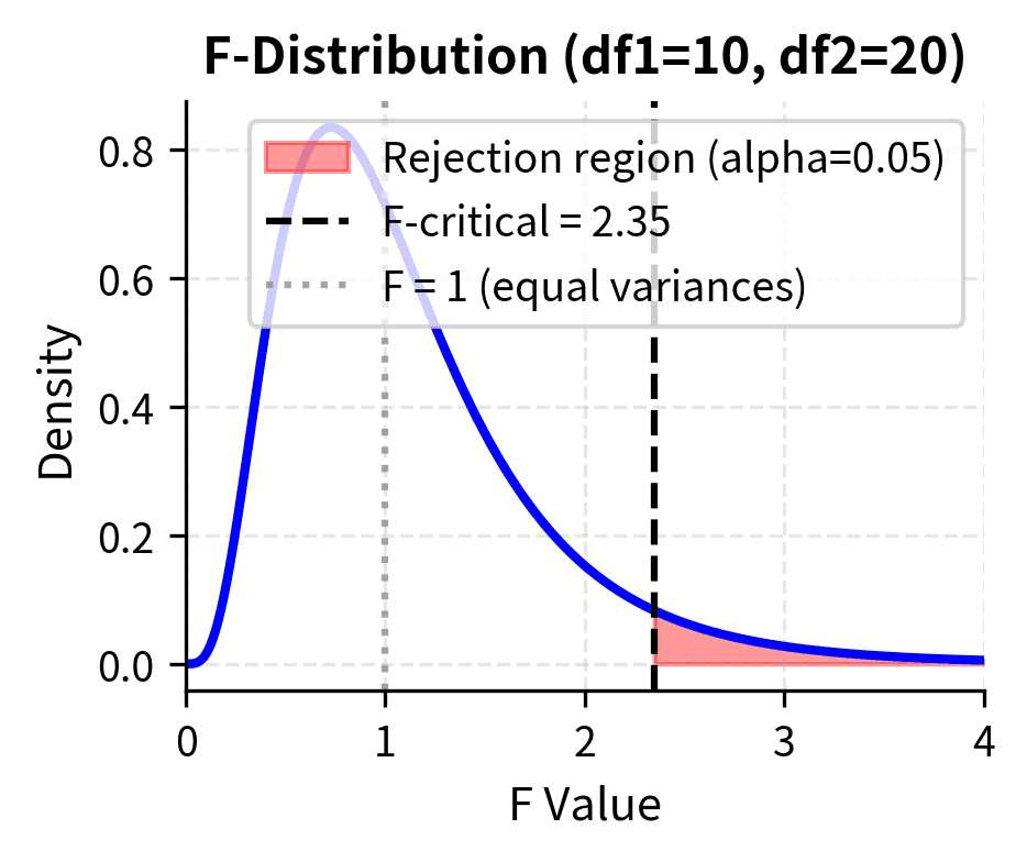
By convention, we place the larger variance in the numerator so that . Under the null hypothesis that , this ratio follows an F-distribution with and . If the true variances are equal, F should be close to 1; values much larger than 1 suggest the numerator variance is genuinely larger.
The degrees of freedom reflect the information available for estimating each variance. Larger samples provide more reliable variance estimates, leading to F-ratios that cluster more tightly around 1 under the null hypothesis. This is captured by the F-distribution becoming less dispersed as both degrees of freedom increase.
When testing whether variances are different (not specifically whether one is greater), you can use a two-tailed test. However, since the F-distribution is not symmetric, you cannot simply double the one-tailed p-value. Instead, calculate the probability of observing an F-ratio as extreme as observed in either direction: .
F-Test in ANOVA: Comparing Multiple Group Means
The most common application of the F-test is in Analysis of Variance (ANOVA), which extends the two-sample t-test to compare means across three or more groups simultaneously. ANOVA is one of the most widely used statistical techniques in experimental research, from agricultural field trials (where it originated) to clinical trials, psychology experiments, and A/B/C testing in technology.
The need for ANOVA arises from a fundamental problem with multiple comparisons. Suppose you want to compare the effectiveness of four different treatments. You might be tempted to conduct all pairwise t-tests: treatment 1 vs. 2, treatment 1 vs. 3, treatment 1 vs. 4, treatment 2 vs. 3, and so on. With four groups, that's 6 separate tests. Even if all treatments are equally effective (the null is true), you would reject at least one comparison about 26% of the time at , not the 5% you might expect. This inflation of Type I error becomes worse with more groups.
ANOVA solves this problem by testing the omnibus null hypothesis that all group means are equal, using a single test that controls the overall Type I error rate.
The Logic of ANOVA
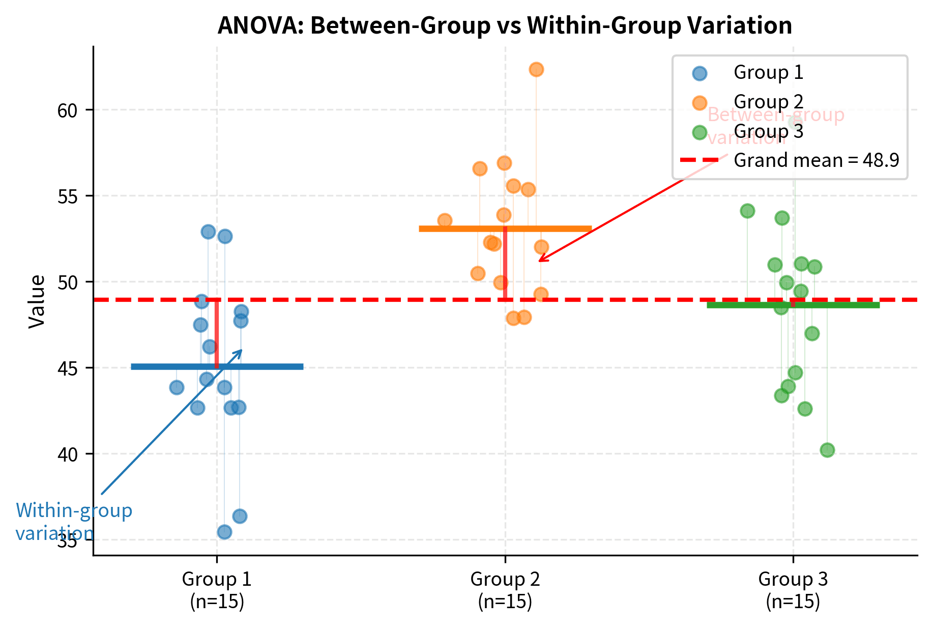
The genius of ANOVA lies in its approach: instead of directly comparing means, it compares variances. This might seem counterintuitive. How does comparing variances tell us about means? The logic is elegant once you understand it.
ANOVA compares two sources of variation:
-
Between-group variance: How much the group means differ from the overall mean. If the null hypothesis is true (all population means are equal), the observed differences among group means reflect only random sampling variation. If the null is false (some means differ), the group means will be more spread out than sampling variation alone would predict.
-
Within-group variance: How much individual observations vary around their group means. This is the baseline variability inherent in the data, driven by individual differences and measurement error. Importantly, this within-group variance is unaffected by whether the population means are equal or different. It measures the "noise" in our data.
If the null hypothesis is true (all population means are equal), both variance estimates should be similar, yielding an F-ratio near 1. The between-group variance just reflects the random sampling variation of means, which should be comparable to what we'd expect given the within-group variability.
If the group means truly differ, the between-group variance will be inflated relative to the within-group variance, producing a large F-ratio. The group means will be more spread out than we'd expect from chance alone, and this excess spread is evidence that the population means differ.
The F-statistic for one-way ANOVA is:
where:
- : the ANOVA F-statistic, the ratio of between-group to within-group variance
- : mean square between groups (variance of group means around the grand mean)
- : mean square within groups (pooled variance within each group)
- : sum of squares between groups, measuring how spread out the group means are
- : sum of squares within groups, measuring variation within each group
- : the number of groups
- : the total sample size across all groups
- : the sample size of group
- : the mean of group
- : the overall (grand) mean of all observations
- : the -th observation in group
- : degrees of freedom for between-group variance
- : degrees of freedom for within-group variance
The intuition is that if group means truly differ, the between-group variance will be large relative to the within-group variance, producing a large F value.
Performing One-Way ANOVA
Let's work through a complete ANOVA example. Suppose we want to test whether three different fertilizers produce different plant growth.
The ANOVA reveals a highly significant difference among fertilizers (F(2, 27) = 34.62, p < 0.001). The effect size η² = 0.72 indicates that 72% of the variation in plant growth is explained by the fertilizer type, representing a large effect.
Post-Hoc Tests: Which Groups Differ?
When ANOVA rejects the null hypothesis, we know at least one group differs, but not which specific groups differ from each other. Post-hoc tests make pairwise comparisons while controlling the family-wise error rate.
Tukey's Honest Significant Difference (HSD) is the most common post-hoc test for ANOVA:
Assumptions of ANOVA
ANOVA relies on similar assumptions to the t-test:
- Independence: Observations within and between groups are independent.
- Normality: Data within each group should be approximately normally distributed.
- Homogeneity of variance: All groups should have similar variances (homoscedasticity).
Levene's test can check the equal variance assumption:
When the equal variance assumption is violated, use Welch's ANOVA (available as scipy.stats.alexandergovern) or the nonparametric Kruskal-Wallis test (scipy.stats.kruskal).
F-Test in Regression: Overall Model Significance
Another crucial application of the F-test is assessing the overall significance of a regression model. The F-test compares the variance explained by the model to the unexplained (residual) variance.
In multiple regression, the F-statistic tests whether any of the predictor variables have a significant relationship with the response variable:
where:
- : the overall F-statistic for the regression model
- : sum of squares explained by the model (variance captured by predictors)
- : sum of squares not explained by the model (remaining variance)
- : mean square for regression (variance explained per predictor)
- : mean square for residuals (unexplained variance per residual df)
- : the number of predictor variables (excluding intercept)
- : the total number of observations
- : residual degrees of freedom
The null hypothesis is that all regression coefficients (except the intercept) are zero, meaning none of the predictors help explain the response.
Comparing Nested Models: F-Test for Model Comparison
The F-test can also compare two nested regression models to determine whether additional predictors significantly improve the model. A model is "nested" within another if it is a special case obtained by setting some coefficients to zero.
where:
- : the F-statistic for comparing nested models
- : residual sum of squares for the simpler (reduced) model
- : residual sum of squares for the complex (full) model with additional predictors
- : residual degrees of freedom for the reduced model
- : residual degrees of freedom for the full model
- : the number of additional predictors being tested
The numerator measures the improvement (reduction in residual SS) per additional predictor, while the denominator estimates the variance of unexplained variation. This tests whether the reduction in residual sum of squares from adding the extra predictors is statistically significant.
The F-test correctly identifies that x₂ (which has a true effect) significantly improves the model, while x₃ (pure noise) does not.
Summary: When to Use the F-Test
The F-test is appropriate for:
- Comparing two variances: Testing whether two populations have equal variability
- ANOVA: Comparing means across three or more groups
- Regression overall significance: Testing whether any predictors have explanatory power
- Nested model comparison: Testing whether additional predictors improve a model
- Testing multiple coefficients simultaneously: Testing whether a subset of regression coefficients are all zero
The F-test is sensitive to violations of normality, particularly in small samples. When normality is questionable, consider nonparametric alternatives such as:
- Levene's test or Brown-Forsythe test for comparing variances (more robust than F-test)
- Kruskal-Wallis test as a nonparametric alternative to one-way ANOVA
- Bootstrap methods for inference on variance ratios
Type I and Type II Errors
Hypothesis testing involves making decisions under uncertainty, which inevitably leads to the possibility of errors. Every time you draw a conclusion from data, you might be wrong. What separates statistical inference from mere guessing is that we can quantify how often we will be wrong and control these error rates through careful study design.
Understanding these errors, their probabilities, and the tradeoffs between them is essential for designing studies and interpreting results. The two error types represent fundamentally different kinds of mistakes with potentially very different consequences.
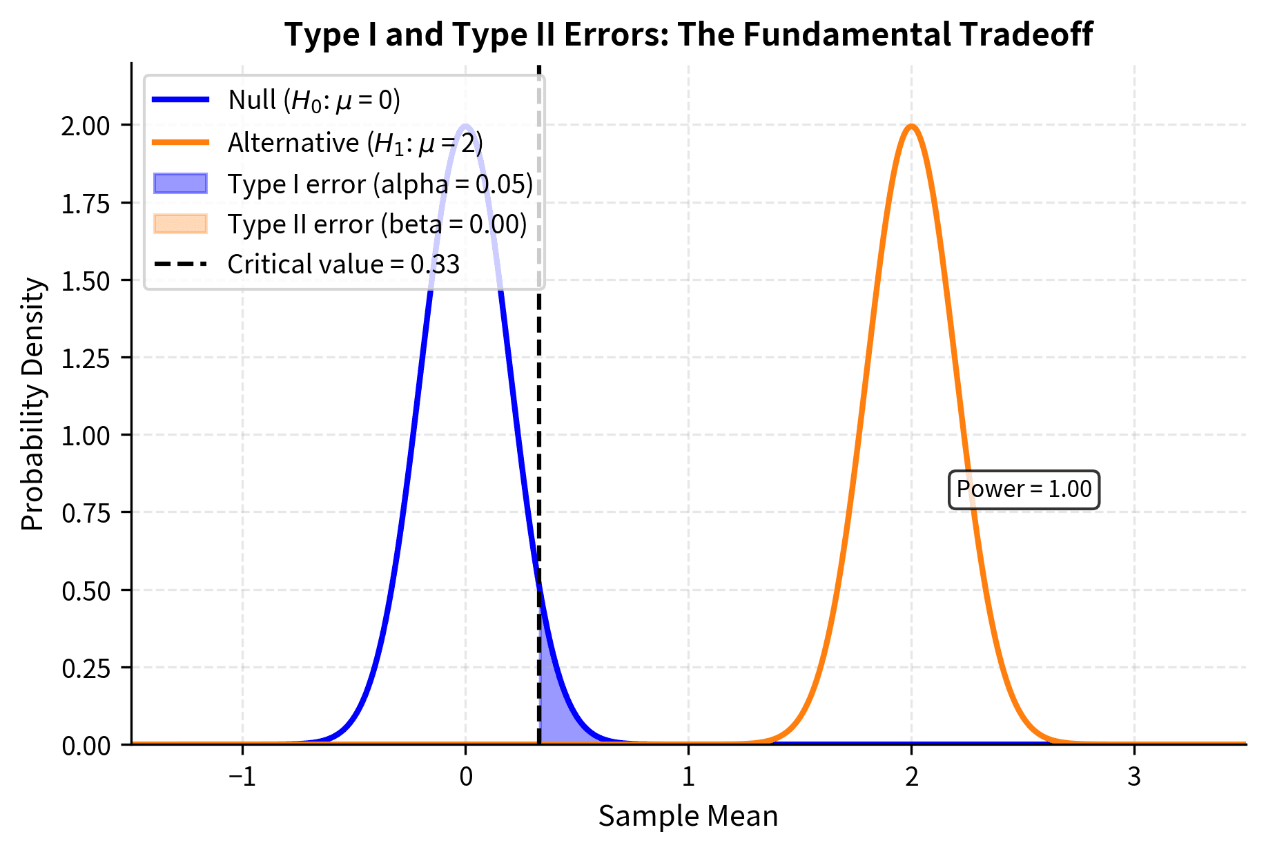
α: False Positive Rate
A Type I error occurs when you reject a true null hypothesis. You conclude that an effect exists when, in reality, nothing is going on. This is a false positive: a false alarm that claims discovery where there is none.
Consider some examples of Type I errors in practice:
- Medical testing: Telling a healthy patient they have a disease (when they don't)
- Quality control: Stopping a manufacturing line that is actually operating correctly
- A/B testing: Deploying a new feature that doesn't actually improve metrics
- Scientific research: Publishing a "discovery" that is just random noise
The probability of a Type I error is denoted and equals the significance level you choose for the test. When you set , you accept a 5% chance of falsely rejecting the null hypothesis when it is true. This is the maximum false positive rate you tolerate.
The key insight is that the significance level is under your direct control. You choose before conducting the test based on the consequences of false positives in your specific context. Contexts where false positives are costly (such as approving an ineffective drug with side effects or claiming a scientific discovery that cannot be replicated) warrant lower significance levels. Particle physics famously uses a 5-sigma threshold (approximately ) before claiming a discovery, reflecting the high stakes of false claims.
β: False Negative Rate
A Type II error occurs when you fail to reject a false null hypothesis. A real effect exists, but your test fails to detect it. This is a false negative: missing a genuine discovery.
Consider some examples of Type II errors in practice:
- Medical testing: Telling a sick patient they are healthy (missing a diagnosis)
- Quality control: Continuing production when the machine is actually malfunctioning
- A/B testing: Abandoning a feature that would actually improve metrics
- Scientific research: Missing a real phenomenon because your study was too small
The probability of a Type II error is denoted . Unlike , which you choose directly, depends on several factors:
- The true effect size: Larger effects are easier to detect. A drug that cuts mortality in half is easier to detect than one that reduces it by 2%.
- The sample size: Larger samples provide more power to detect effects. With more data, genuine patterns emerge from the noise.
- The significance level: Lower means higher , all else equal. Being more stringent about false positives makes you more likely to miss true positives.
- The population variance: Less variable populations yield more precise estimates. If individual responses are highly variable, it's harder to detect systematic differences.
You do not directly set , but you can influence it through study design, particularly by choosing an adequate sample size. This is why power analysis is a critical part of study planning.
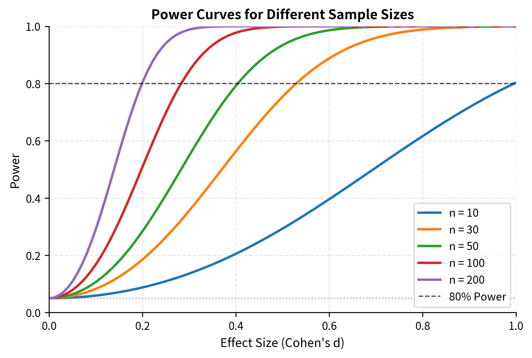
Power: The Probability of Detecting Real Effects
Statistical power is defined as : the probability of correctly rejecting the null hypothesis when it is false. Power represents the sensitivity of your test to detect real effects that actually exist.
Think of power as the "detection rate" of your study. If a genuine effect exists, power tells you the probability that your study will find it. A study with 80% power has an 80% chance of detecting a true effect and a 20% chance of missing it.
High power is desirable because it means you are likely to find effects that genuinely exist. Low power means you might miss important effects, leading to inconclusive studies and wasted resources. Underpowered studies are a significant problem in research: they fail to detect real effects, contribute to publication bias (because null results are often not published), and waste participants' time and researchers' effort.
The conventional target is 80% power, meaning you have an 80% chance of detecting an effect if it truly exists. Some fields use 90% power for greater assurance. Below 50% power, your study is more likely to miss a true effect than to find it, essentially worse than a coin flip for detecting reality.
The Tradeoff Between Error Types
There is a fundamental tradeoff between Type I and Type II errors. For a fixed sample size, decreasing (being more conservative about false positives) necessarily increases (making false negatives more likely). You cannot simultaneously minimize both error types without increasing your sample size.
This tradeoff means you must weigh the relative costs of each error type for your specific application:
- In criminal trials, the presumption of innocence prioritizes avoiding Type I errors (convicting an innocent person) even at the cost of higher Type II errors (acquitting a guilty person).
- In medical screening for a deadly disease, you might accept more false positives (Type I errors requiring follow-up testing) to minimize false negatives (missing cases of the disease).
- In exploratory research, you might use a liberal significance level to avoid missing potentially important leads, accepting that some will not replicate.
The only way to reduce both error types simultaneously is to increase the sample size, which narrows the sampling distribution and improves your ability to distinguish between the null and alternative hypotheses.
Sample Size and Minimum Detectable Effect
Before conducting a study, you should determine how large a sample you need. Power analysis formalizes this, connecting sample size to your ability to detect effects of a given magnitude.
How n, Variance, α, Power, and Effect Size Connect
The power of a test depends on five interrelated quantities:
- Sample size (n): Larger samples give more power.
- Effect size: Larger true effects are easier to detect.
- Population variance (): Less variability gives more power.
- Significance level (α): Lower α reduces power (more conservative).
- Power (1 - β): The target probability of detecting a true effect.
Given any four of these, you can calculate the fifth. The most common application is solving for sample size given the other quantities:
where:
- : the required sample size
- : the critical value from the standard normal distribution for significance level (e.g., 1.96 for , two-sided)
- : the z-value corresponding to the desired power (e.g., 0.84 for 80% power)
- : the minimum effect size you want to detect (in the original units)
- : the population standard deviation
- : Cohen's d, the standardized effect size
This formula reveals the key tradeoffs in study design: detecting smaller effects () requires larger samples, as does achieving higher power () or using more stringent significance levels (smaller ). Greater population variability () also increases sample size requirements.
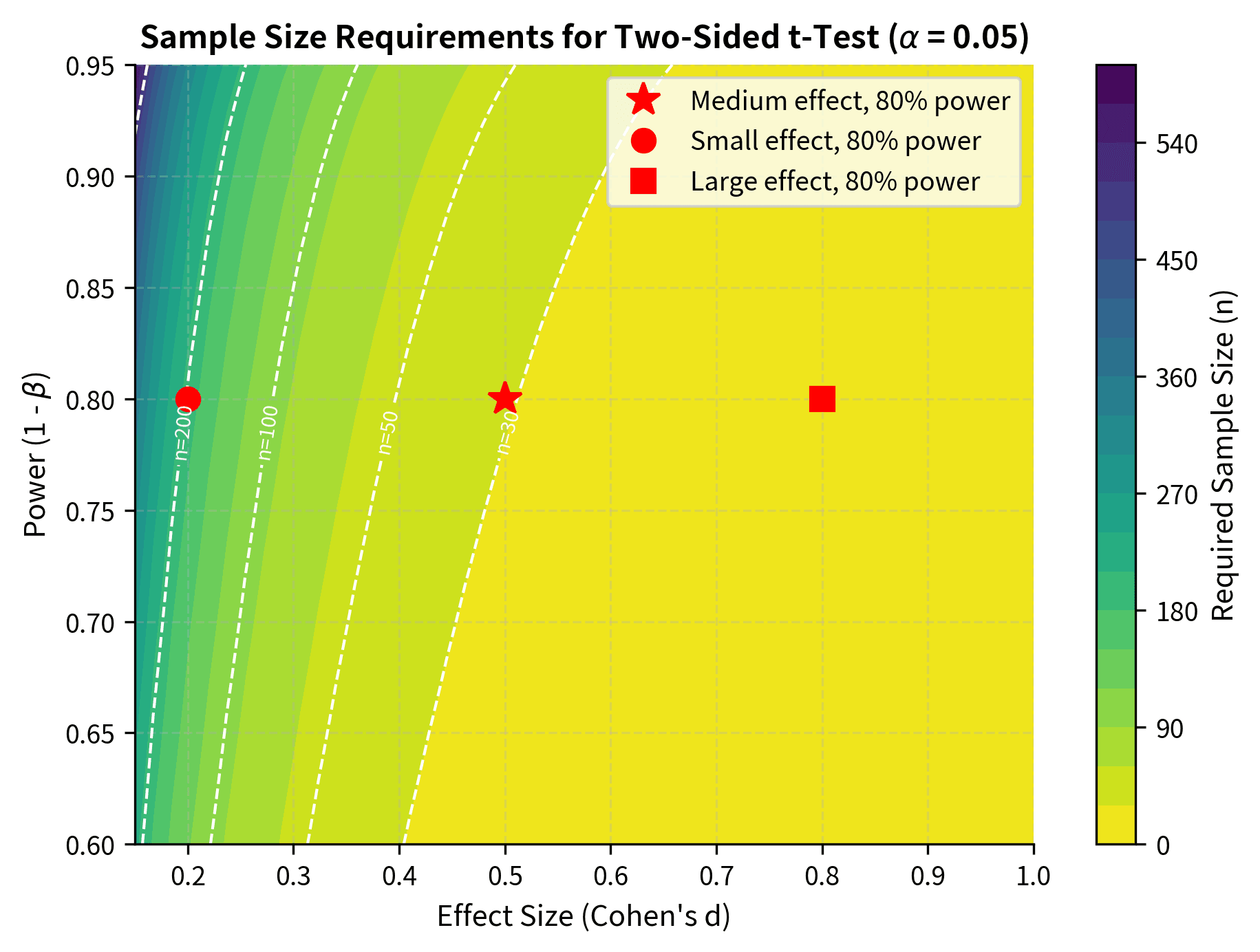
Minimum Detectable Effect (MDE)
The minimum detectable effect (MDE) is the smallest effect size that your study can reliably detect. Given your sample size, variance, significance level, and desired power, the MDE tells you the threshold below which effects will likely go undetected.
MDE is particularly important for A/B testing and experimental design. If your business requires detecting a 2% improvement in conversion rate, you need to ensure your sample size is sufficient to achieve adequate power for that effect size. If your MDE is 5%, you might have high power but would miss smaller improvements that could still be valuable.
Underpowered Studies and "Significance Chasing"
Underpowered studies are those with too few observations to reliably detect effects of the size expected or desired. They have several problematic consequences:
High false negative rates: Real effects are missed because the study lacks sensitivity to detect them.
Inflated effect size estimates: When an underpowered study does achieve statistical significance, the effect size estimate is often inflated. This is because only the studies where random variation pushed the estimate above the significance threshold get published, a phenomenon called the "winner's curse."
Significance chasing: Researchers with underpowered studies may engage in questionable practices to achieve significance: running multiple analyses and reporting only those that "work," adding more observations until significance is reached, or dropping "outliers" selectively. These practices inflate false positive rates and produce unreliable findings.
Planning adequate sample sizes before data collection helps avoid these problems. If a properly powered study is infeasible due to resource constraints, it may be better not to run the study at all than to produce unreliable results.
Effect Sizes: Practical Significance
Statistical significance tells you whether an effect is distinguishable from zero with a specified error rate. It does not tell you whether the effect is large enough to matter in practice. Effect sizes fill this gap by quantifying the magnitude of effects.
Mean Difference and Standardized Difference
The simplest effect size for comparing means is the raw mean difference: . This is directly interpretable in the original units of measurement. If treatment improves response time by 50 milliseconds, that number has immediate practical meaning.
However, raw differences are hard to compare across studies with different scales. Cohen's d standardizes the difference by dividing by the pooled standard deviation:
where:
- : Cohen's d, the standardized effect size
- : the difference between group means
- : the pooled standard deviation, calculated as
Cohen's d expresses the difference in standard deviation units, making it comparable across different measures and studies. A value of d = 0.5 means the groups differ by half a standard deviation, regardless of whether the original scale measures test scores, reaction times, or blood pressure.
Cohen's conventional benchmarks for interpreting d are:
- Small effect: d ≈ 0.2
- Medium effect: d ≈ 0.5
- Large effect: d ≈ 0.8
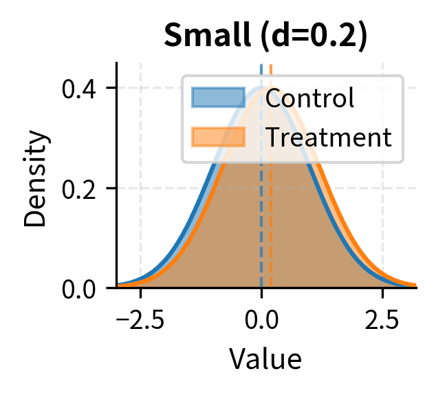
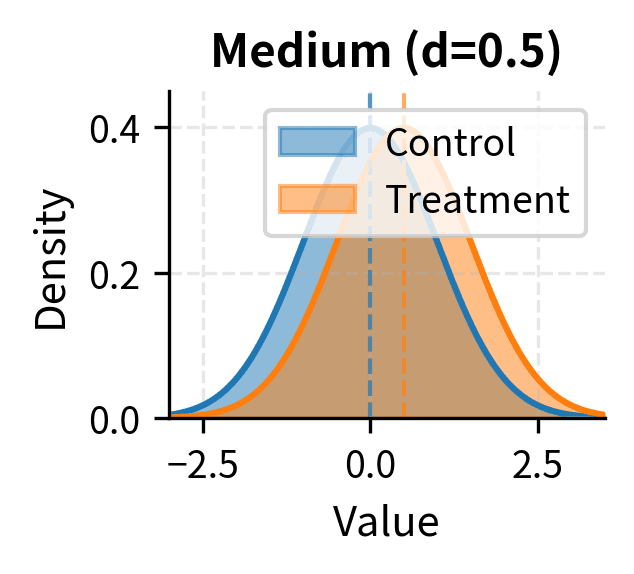
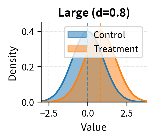
These are rough guidelines, not rigid rules. What counts as a "large" effect depends on the context. A drug that improves survival by d = 0.2 might be clinically important if the alternative is death. A teaching intervention with d = 0.8 might not matter if the cost of implementation is prohibitive.
The treatment group shows a large effect (d = 2.48), meaning the treatment mean is about 2.5 standard deviations above the control mean.
Why Tiny P-values Can Mean Tiny Effects
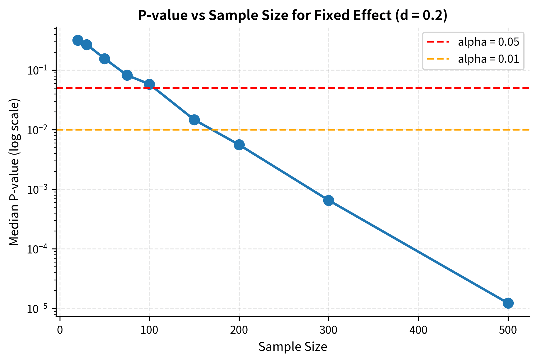
With large enough samples, even trivial effects produce tiny p-values. This is because the standard error decreases as , so the test statistic grows larger for any fixed effect size.
Consider testing whether the average height of a population differs from 170 cm. With a sample of 10,000 people, an observed mean of 170.1 cm would yield a highly significant result (p < 0.001) despite representing a difference of only 0.1 cm, which is practically meaningless.
This is why effect sizes should always accompany p-values. The p-value tells you that an effect exists (with some confidence); the effect size tells you whether that effect is large enough to care about. Both pieces of information are necessary for sound interpretation.
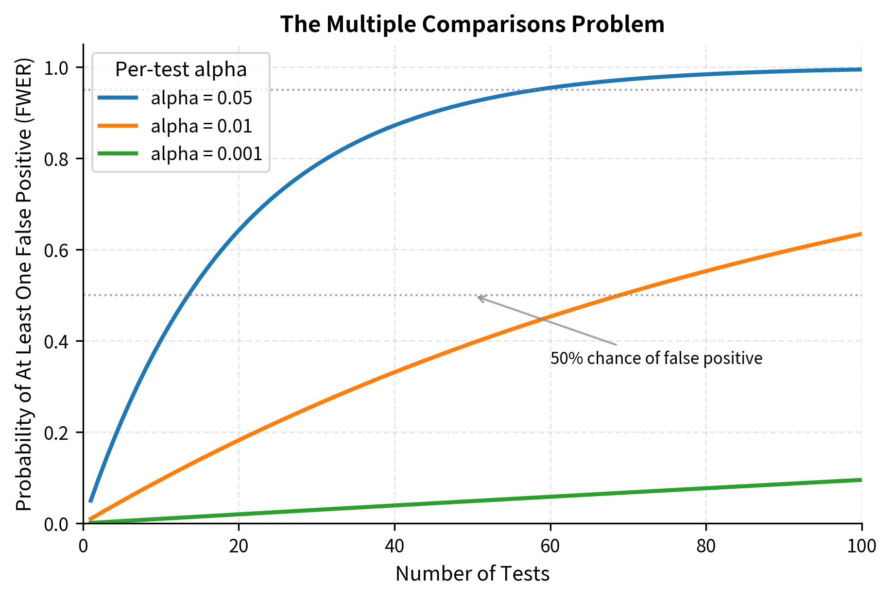
Multiple Comparisons
When you conduct multiple hypothesis tests, the probability of at least one false positive increases dramatically. If you perform 20 independent tests at , the probability of at least one Type I error is , not 0.05. This is the multiple comparisons problem.
Family-Wise Error Rate vs False Discovery Rate
There are two main ways to conceptualize the error rate when conducting multiple tests:
The family-wise error rate (FWER) is the probability of making at least one Type I error among all tests. Controlling the FWER at 0.05 means you have at most a 5% chance of any false positives. This is a conservative approach appropriate when even a single false positive has serious consequences.
The false discovery rate (FDR) is the expected proportion of false positives among the rejected hypotheses. Controlling the FDR at 0.05 means that among the tests you call "significant," about 5% are expected to be false positives. This is a less conservative approach appropriate for exploratory analyses where some false positives are acceptable as long as most discoveries are real.
Correction Methods
Several methods exist for controlling error rates in multiple testing:
Bonferroni correction is the simplest approach to controlling FWER. It adjusts the significance level by dividing by the number of tests: if you conduct tests and want FWER = 0.05, use for each individual test. Equivalently, multiply each p-value by and compare to the original .
Bonferroni is conservative, especially when tests are correlated. With many tests, the adjusted significance level becomes very stringent, potentially missing real effects.
Holm's method is a step-down procedure that is uniformly more powerful than Bonferroni while still controlling FWER. You order p-values from smallest to largest, then compare each to an adjusted threshold that becomes less stringent as you proceed.
Benjamini-Hochberg (BH) procedure controls the FDR rather than the FWER. It is the most common FDR-controlling method:
- Order p-values from smallest to largest:
- Find the largest such that
- Reject all hypotheses with p-values
This method is less conservative than Bonferroni and is widely used in genomics, neuroimaging, and other fields with many simultaneous tests.
With 10 tests, Bonferroni requires p < 0.005 for significance, rejecting only 2 hypotheses. Benjamini-Hochberg, controlling FDR instead of FWER, rejects 5 hypotheses. The choice between methods depends on whether you prioritize avoiding any false positives (Bonferroni/Holm) or maximizing discoveries while controlling their expected proportion (BH).
Practical Reporting and Interpretation
Good statistical practice involves more than calculating test statistics and p-values. Clear, complete reporting enables readers to evaluate your conclusions and, if necessary, combine your results with other evidence.
What to Report
A complete statistical report includes:
- The estimate: The sample statistic (mean, difference, correlation) that estimates the population parameter.
- A confidence interval: The range of plausible values for the parameter, conveying uncertainty.
- The p-value: The exact p-value (not just "p < 0.05"), enabling readers to assess evidence strength.
- The test used: Specify whether you used a t-test, z-test, Welch's test, etc.
- Key assumptions: State whether you assessed normality, equal variances, independence, and what you found.
- Effect size: Report standardized effect sizes when appropriate for comparability.
For example, a complete report might read: "The treatment group (M = 89.2, SD = 2.7) scored significantly higher than the control group (M = 81.1, SD = 2.8), t(18) = 6.47, p < 0.001, 95% CI for the difference [5.5, 10.7], Cohen's d = 2.48. The assumption of equal variances was supported by Levene's test (p = 0.82)."
Avoiding Misleading Language
Avoid language that overstates conclusions:
- Don't say "The treatment works" or "The groups are different." Say "The data provide evidence that..." or "We observed a difference in..."
- Don't equate "not significant" with "no effect." Absence of evidence is not evidence of absence, especially in underpowered studies.
- Don't use p-values as measures of effect size. A highly significant result (p = 0.0001) is not necessarily a large effect.
- Don't interpret non-significant results as "confirming the null hypothesis." You failed to reject it, which is different from proving it true.
Statistical significance is a technical term with a precise meaning. In everyday language, "significant" implies "important" or "meaningful." Statistically significant results may be neither. Use precise language that distinguishes between statistical and practical significance, and always consider whether your statistically significant findings are large enough to matter in context.
Summary
Hypothesis testing provides a rigorous framework for making decisions about populations based on sample data. The p-value, properly understood, quantifies how surprising your data would be if the null hypothesis were true. It is not the probability that the null hypothesis is true, nor does it measure effect size. The conventional threshold of 0.05 is arbitrary, and results should be interpreted on a continuum of evidence.
Setting up a hypothesis test requires specifying null and alternative hypotheses, choosing between one-sided and two-sided tests based on the research question, and understanding how test statistics relate to sampling distributions. Confidence intervals and hypothesis tests are mathematically equivalent, with confidence intervals providing the added benefit of showing the range of parameter values consistent with your data.
The choice between z-tests and t-tests depends on whether the population standard deviation is known. In practice, use t-tests unless you have genuine prior knowledge of . Welch's t-test is the safer default for comparing two groups, as it maintains validity when variances are unequal without substantial loss of power when they are equal.
Type I and Type II errors represent the two ways hypothesis tests can go wrong. The tradeoff between them means you cannot minimize both without increasing sample size. Power analysis helps you plan studies with adequate sensitivity to detect effects of meaningful magnitude. Effect sizes complement p-values by quantifying the magnitude of effects, preventing the conflation of statistical and practical significance.
When conducting multiple tests, use appropriate corrections to control error rates. The choice between FWER-controlling methods like Bonferroni and FDR-controlling methods like Benjamini-Hochberg depends on the relative costs of false positives and false negatives in your application.
Finally, good reporting practice requires complete information: estimates, confidence intervals, exact p-values, test specifications, assumption checks, and effect sizes. This transparency enables readers to evaluate your conclusions and builds the foundation for cumulative scientific knowledge.
Key Parameters
This section summarizes the critical parameters for hypothesis testing and how to select appropriate values for your analyses.
Significance Level (α)
The probability threshold for rejecting the null hypothesis.
- Default: 0.05 (5% false positive rate)
- More stringent: 0.01 or 0.001 for high-stakes decisions (drug approval, major scientific claims)
- More lenient: 0.10 for exploratory analyses where missing effects is costly
- Guidance: Choose before seeing data based on consequences of Type I errors
Power (1 - β)
The probability of detecting a true effect when it exists.
- Standard target: 0.80 (80% chance of detecting a real effect)
- High-powered studies: 0.90 or 0.95 for confirmatory research
- Guidance: Higher power requires larger samples; balance against practical constraints
Effect Size Thresholds (Cohen's d)
Standardized measure of the difference between groups.
- Small: d ≈ 0.2 (subtle effects, may require large samples to detect)
- Medium: d ≈ 0.5 (noticeable effects, typical in social sciences)
- Large: d ≈ 0.8 (substantial effects, easily detected with modest samples)
- Guidance: Define the minimum practically meaningful effect for your domain
Test Selection Parameters
| Scenario | σ Known? | Groups | Recommendation |
|---|---|---|---|
| One sample, population σ known | Yes | 1 | Z-test |
| One sample, population σ unknown | No | 1 | One-sample t-test |
| Two independent samples, equal variances | No | 2 | Pooled t-test (or default to Welch's) |
| Two independent samples, unequal/unknown variances | No | 2 | Welch's t-test |
| Paired/matched observations | No | 2 (paired) | Paired t-test |
| Comparing variances | N/A | 2 | F-test (or Levene's for robustness) |
| Multiple groups | No | ≥3 | One-way ANOVA |
Multiple Comparison Corrections
When conducting multiple tests, choose a correction method:
- Bonferroni: Simple, conservative; use when any false positive is costly
- Holm's method: Step-down procedure, more powerful than Bonferroni while controlling FWER
- Benjamini-Hochberg: Controls FDR; use for exploratory analyses with many tests
scipy.stats Functions
| Test Type | Function | Key Parameters |
|---|---|---|
| One-sample t-test | ttest_1samp(a, popmean) | a: sample data, popmean: hypothesized mean |
| Two-sample t-test | ttest_ind(a, b, equal_var) | equal_var=False for Welch's t-test |
| Paired t-test | ttest_rel(a, b) | Paired samples as two arrays |
| One-way ANOVA | f_oneway(*groups) | Pass each group as separate argument |
| Levene's test | levene(*groups) | Tests equality of variances |
| Shapiro-Wilk | shapiro(x) | Tests normality assumption |
Quiz
Ready to test your understanding? Take this quick quiz to reinforce what you've learned about hypothesis testing, p-values, and statistical inference.


Comments