PEFT Motivation: Why Parameter-Efficient Fine-Tuning Matters

In Part XXIV, we explored full fine-tuning: updating all parameters of a pre-trained model to adapt it for a specific downstream task. Full fine-tuning produces excellent results, but as models have grown from millions to billions of parameters, a practical problem has emerged. Training, storing, and deploying a separate 70-billion-parameter model for each task becomes prohibitively expensive. Parameter-Efficient Fine-Tuning (PEFT) addresses this by updating only a small fraction of parameters while keeping most of the model frozen.

This chapter examines why PEFT has become essential for modern LLM deployment. We'll quantify the storage and compute costs of full fine-tuning at scale, explore the challenges of serving multiple specialized models, and understand the trade-offs between parameter efficiency and task performance. This foundation prepares us for the specific PEFT techniques covered in subsequent chapters, including LoRA, prefix tuning, and adapter layers.

Modern language models contain billions of parameters, each stored as a floating-point number. Every weight in a neural network occupies physical memory on a GPU or in system RAM. When you multiply billions of parameters by the bytes required for each floating-point representation, the resulting storage requirements quickly reach sizes that strain even enterprise-grade hardware. Understanding these raw storage costs reveals why full fine-tuning doesn't scale to practical deployment scenarios.

Before we can appreciate the need for parameter efficiency, we must first establish a clear picture of how much space these models actually consume. The storage footprint depends on two factors: the number of parameters in the model and the numerical precision used to represent each parameter. Common precision formats include FP32 (32-bit floating point, requiring 4 bytes per parameter), FP16 and BF16 (16-bit formats, requiring 2 bytes each), and quantized formats like INT8 (1 byte) or INT4 (half a byte). Let's calculate the storage requirements for popular LLM architectures across these different precision levels:

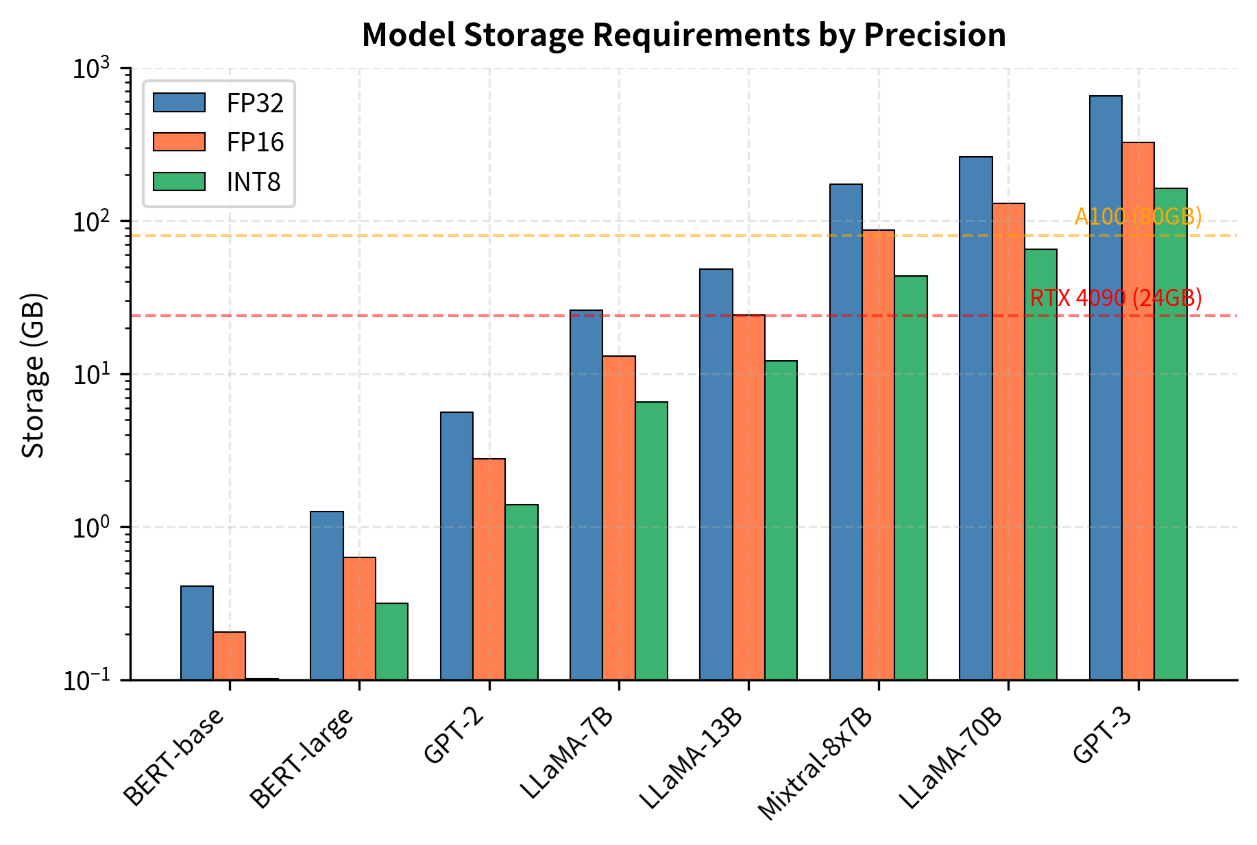
The numbers illustrate the challenge clearly. A single LLaMA-70B model requires 130 GB in FP16 precision, which is the standard format for fine-tuning since it balances numerical stability with memory efficiency. Even with aggressive INT8 quantization, you still need 65 GB just for model weights. To put this in perspective, a high-end consumer GPU like the NVIDIA RTX 4090 has only 24 GB of memory, meaning even quantized versions of these large models cannot fit on typical hardware. This storage requirement represents just the static weights, before we consider the additional memory needed during training or inference.

The storage challenge described above represents the cost for a single model, but real-world deployments rarely involve just one task. Organizations typically need models specialized for multiple applications: customer support chatbots, code assistants, document summarization tools, and more. With full fine-tuning, each task requires its own complete copy of the model, causing storage requirements to multiply linearly with the number of tasks. Consider a company deploying LLMs for several applications:

The multiplication effect becomes dramatic at scale. Deploying eight task-specific LLaMA-70B models requires over 1 TB of storage for weights alone. This calculation doesn't even include optimizer states, activation checkpoints, or the redundant copies needed for high availability in production systems. At the enterprise level, where organizations might have dozens of specialized applications, the storage infrastructure costs become prohibitive. This linear scaling with task count represents a fundamental limitation of the full fine-tuning paradigm.

Storage is only part of the problem. While storage determines how many models you can save to disk, training memory determines whether you can update those models at all. The training process requires substantially more memory than inference because the GPU must simultaneously hold the model parameters, the gradients computed during backpropagation, and the optimizer states that track momentum and variance for each parameter. Each of these components consumes memory proportional to the parameter count:

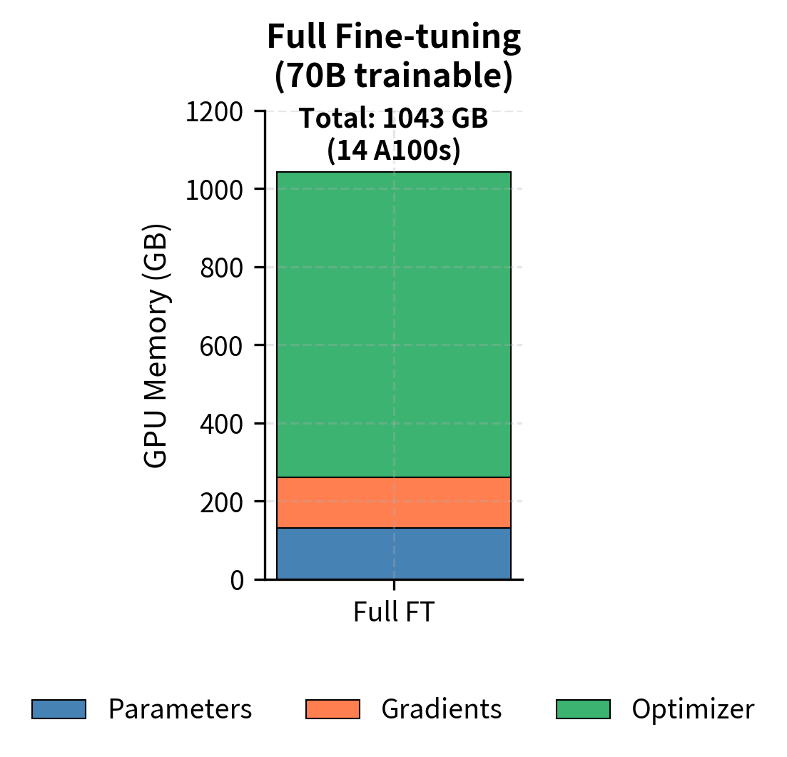
Let's examine how these components contribute to the total memory footprint. The model parameters themselves require storage proportional to their precision. Gradients, computed during the backward pass, require the same amount of memory since each parameter receives a corresponding gradient value. The optimizer states for AdamW are particularly memory-intensive because the algorithm maintains two running averages (momentum and variance) for each parameter, typically stored in full FP32 precision to ensure numerical stability. When training in mixed precision (FP16 or BF16), the optimizer also maintains a master copy of the weights in FP32 for accurate weight updates.

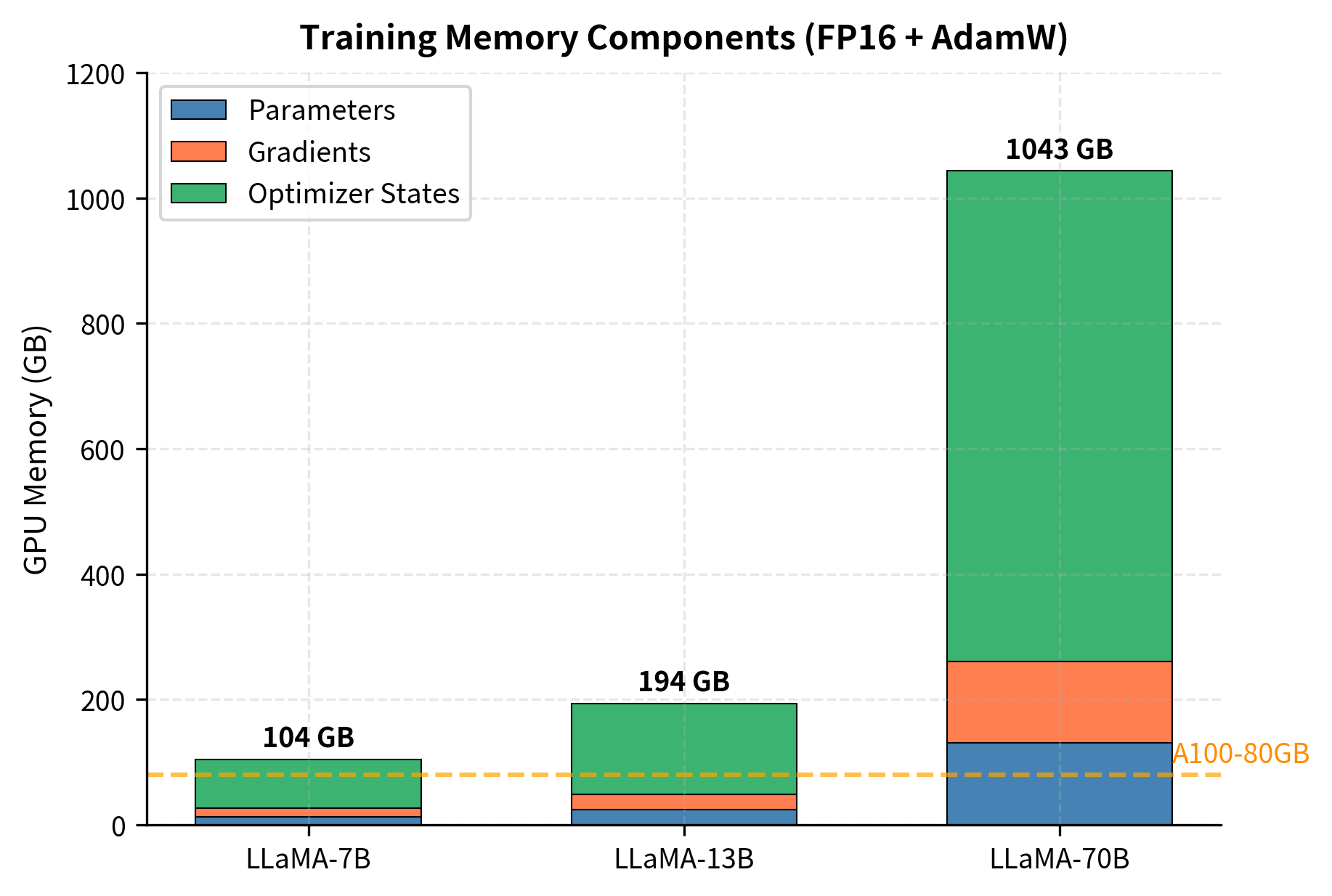
The memory requirements for training are substantial. Full fine-tuning of LLaMA-70B requires approximately 1,040 GB of GPU memory for parameters, gradients, and optimizer states alone. To understand what this means in practice, consider that a single A100 GPU, one of the most powerful GPUs available for machine learning, has 80 GB of memory. Simple arithmetic reveals that you need at least 14 A100 GPUs just for these components, before accounting for the activation memory required to store intermediate values during the forward pass. This hardware requirement places full fine-tuning of large models out of reach for you and most organizations.

Beyond storage costs, serving multiple fine-tuned models creates operational complexity that impacts latency, throughput, and infrastructure costs.

When deploying multiple task-specific models, you face architectural decisions that trade off between resource usage and response latency:

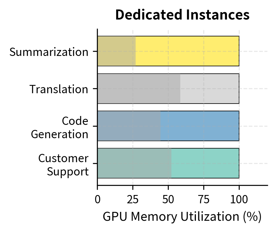
Dedicated instances assign one GPU (or GPU cluster) per task-specific model:

• Consistent low latency since models are always loaded
• Poor resource utilization during low-traffic periods
• Linear cost scaling: 8 tasks × N GPUs per model

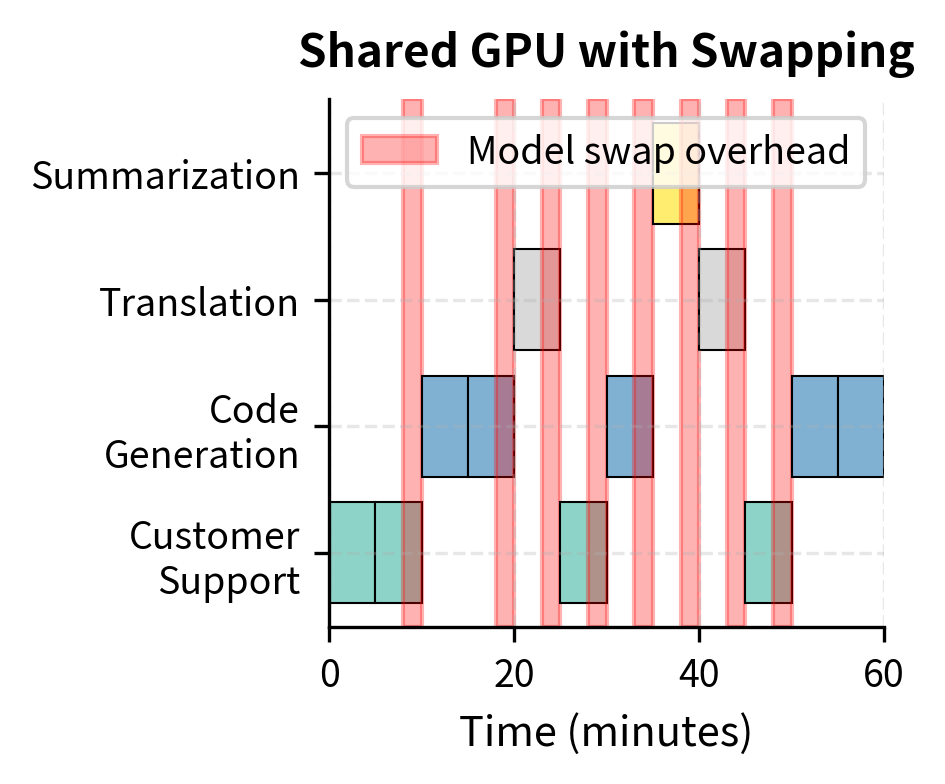
Shared infrastructure with model swapping loads models on-demand:

• Better utilization during variable traffic
• Introduces 30-60 second swap latency for large models
• Complex orchestration to predict traffic patterns

Neither approach handles multi-task deployment gracefully when each task requires a complete model copy.

Modern GPU clusters typically provision 8-16 GPUs per node, with each GPU containing 40-80 GB of memory. Let's visualize how quickly this fills up:

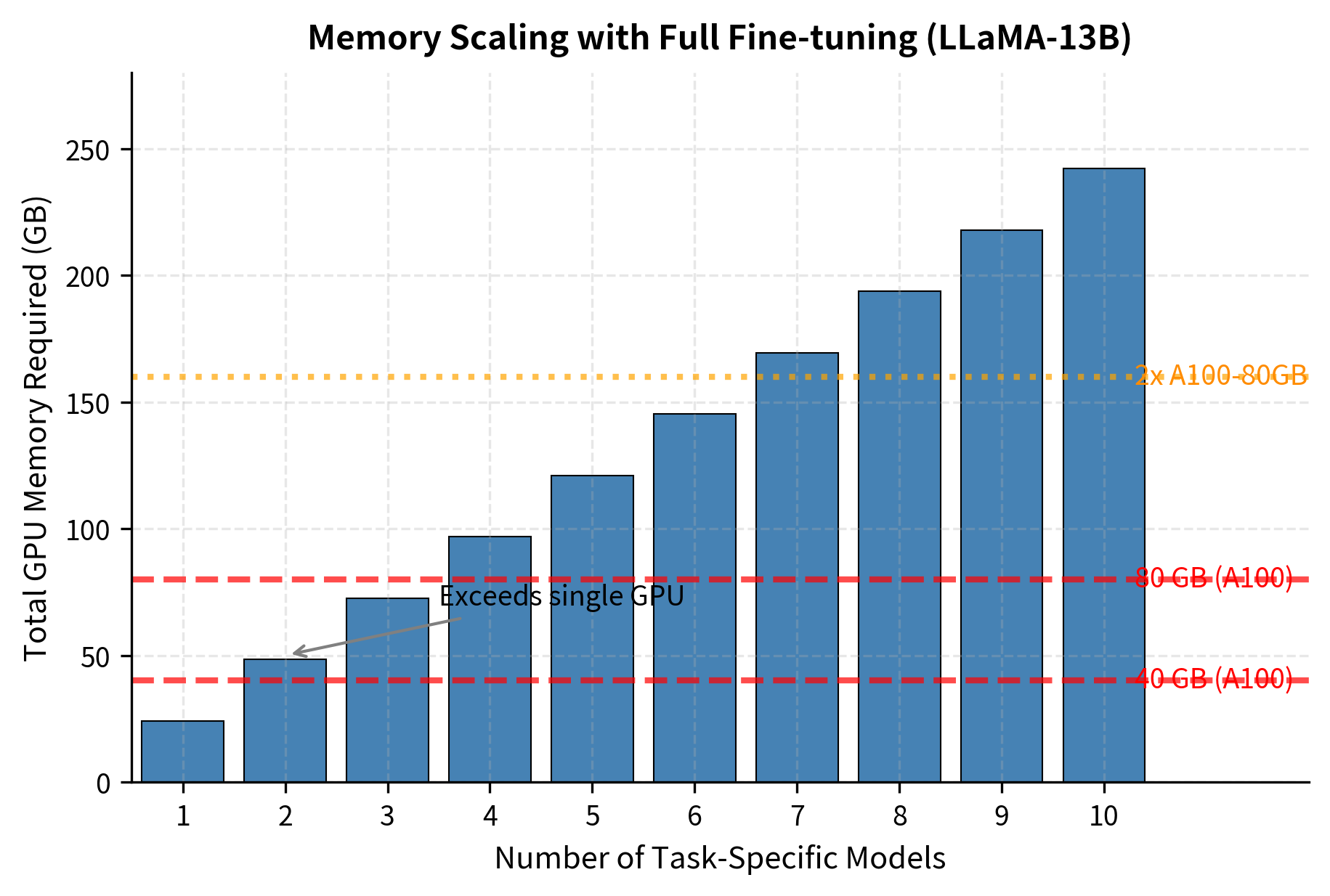
With LLaMA-13B, you can fit only one or two task-specific models on a single A100-80GB GPU. Scaling to eight tasks requires distributed serving or expensive model swapping.

The challenges outlined above, including the storage multiplication problem, the enormous training memory requirements, and the operational complexity of serving multiple large models, point toward a fundamental question: is it really necessary to modify every single parameter to adapt a model to a new task? Parameter-efficient fine-tuning offers a fundamentally different approach: instead of modifying all model weights, train only a small number of additional parameters while keeping the pre-trained weights frozen. This insight, that task adaptation can be achieved through targeted modifications rather than wholesale changes, forms the conceptual foundation for all PEFT methods.

The core principle behind PEFT's storage efficiency is strikingly simple. Rather than creating independent copies of the entire model for each task, PEFT stores a single copy of the base model and supplements it with small, task-specific adapter modules. These adapters typically modify less than 1% of total parameters, yet they capture the task-specific knowledge needed for strong performance. This architectural decision fundamentally changes the storage equation from a multiplicative relationship to an additive one. Let's quantify exactly how dramatic this change becomes:

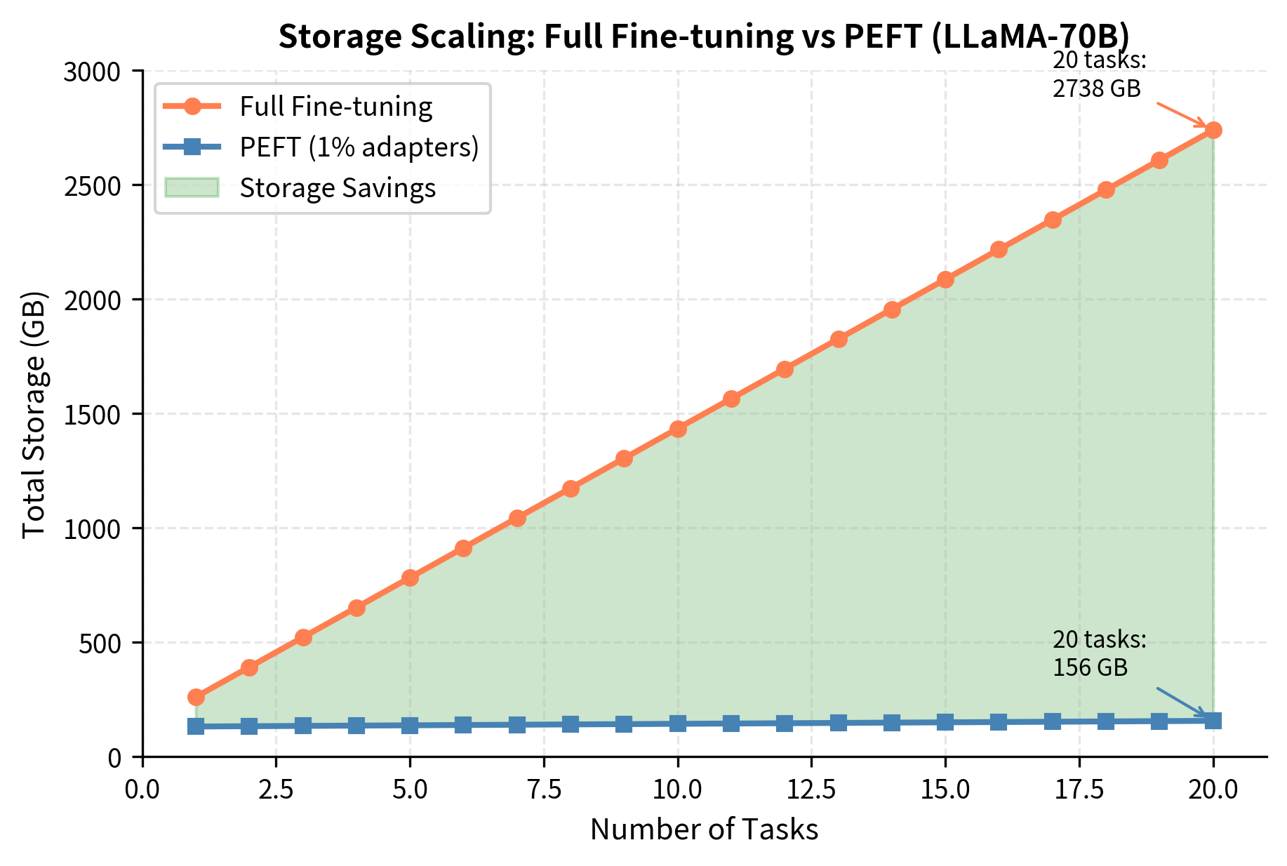
The mathematics of PEFT storage reveals why this approach scales so well. With full fine-tuning, total storage grows as $S_{full} = (N_{tasks} + 1) \times S_{model}$, where each task adds an entire model's worth of storage. With PEFT, total storage follows a different formula: $S_{PEFT} = S_{model} + N_{tasks} \times S_{adapter}$. Since the adapter size $S_{adapter}$ is typically only 1% of $S_{model}$, adding more tasks barely increases the total footprint. Let's see this principle in action across different model scales:

The savings are dramatic. With PEFT, deploying eight LLaMA-70B variants requires 140 GB instead of 1,170 GB, over an 8× reduction. The base model is stored once, and each task adds only a small adapter. Notice how the savings ratio improves as we scale to larger models and more tasks, precisely because the adapter overhead becomes proportionally smaller relative to the base model. For organizations deploying dozens of specialized models, these savings translate directly into reduced infrastructure costs and simplified operations.

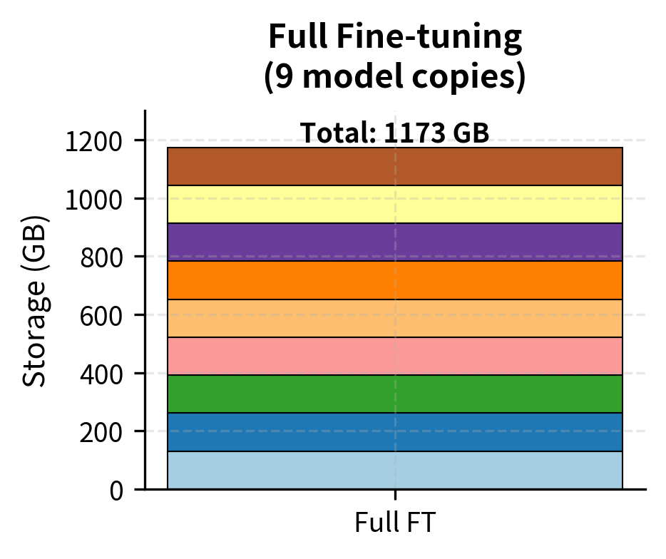
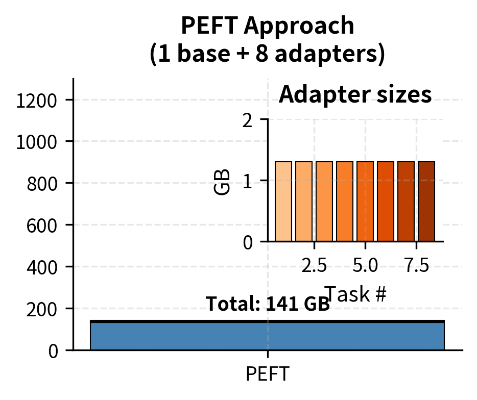
The visualization illustrates how the base model dominates the storage footprint in PEFT, whereas full fine-tuning replicates the massive model for every task. The inset panel zooms in on the adapter sizes, revealing that all eight task-specific adapters combined occupy less space than a single percentage point of the base model. This visual contrast underscores the scalability advantage of the PEFT approach.

PEFT reduces training costs beyond just storage. The key insight is that with fewer trainable parameters, you need less GPU memory because gradients and optimizer states only accumulate for the parameters that actually require updates. The frozen base model participates in the forward pass to compute activations, but it does not need gradient storage or optimizer state tracking. This selective allocation of training resources produces substantial memory savings:

Notice how this function distinguishes between frozen and trainable parameters. The frozen parameters, comprising 99% of the model, require only storage for their weights. They flow through the forward computation but contribute nothing to the backward pass's memory footprint. In contrast, the trainable parameters, though representing only 1% of the total, carry the full burden of gradients and optimizer states. This asymmetric treatment is what enables the dramatic memory reduction.

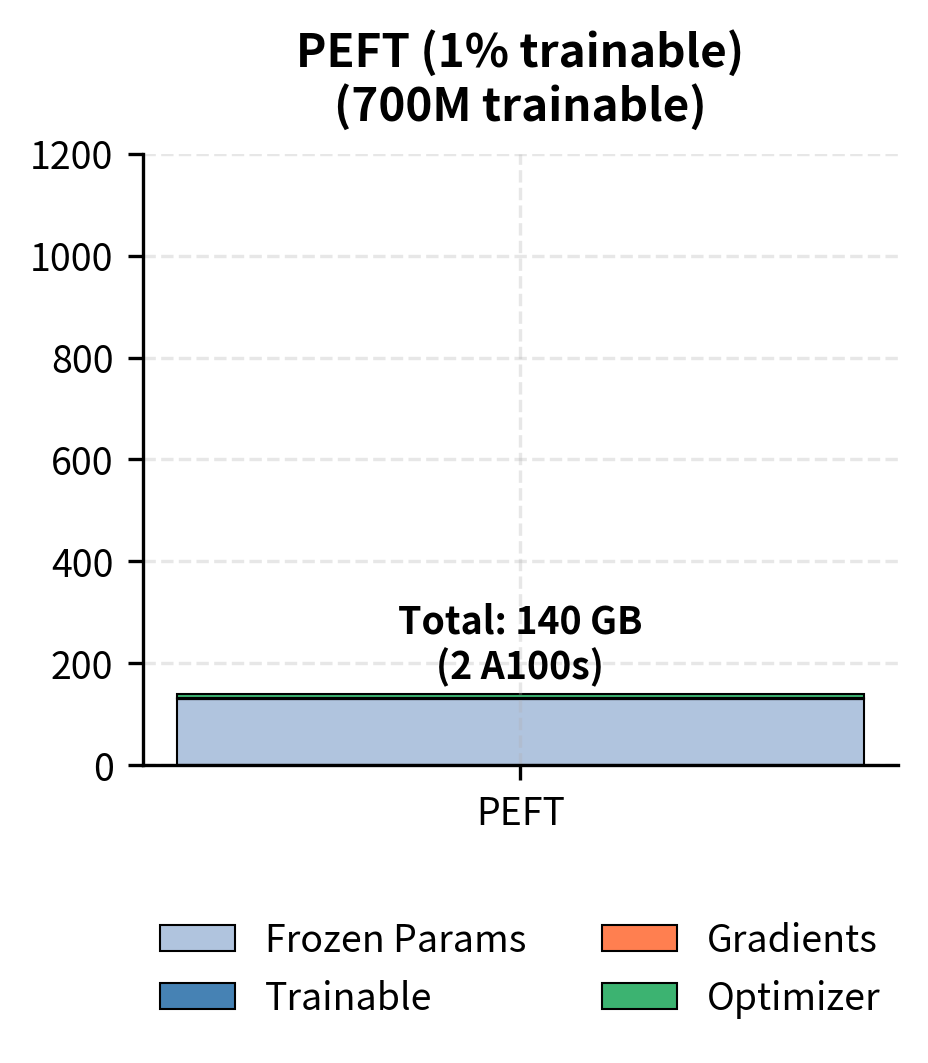
PEFT reduces training memory by roughly 7× for LLaMA-70B, dropping from over 1,000 GB to approximately 140 GB. More importantly, this shifts training from requiring 14+ A100 GPUs to potentially fitting on just 2 GPUs. The practical implications are significant: research labs, startups, and you can now fine-tune state-of-the-art models on hardware you can actually access. This accessibility improvement democratizes fine-tuning of large models, enabling a much broader community to participate in adapting these powerful systems to specialized tasks.

Beyond the training benefits, PEFT enables a powerful deployment pattern: hot-swapping adapters without reloading the base model. In traditional full fine-tuning deployments, switching between tasks requires unloading one multi-gigabyte model from GPU memory and loading another in its place. This process takes 30-60 seconds for large models, creating unacceptable latency for interactive applications. PEFT fundamentally changes this dynamic by decoupling the base model from the task-specific components.

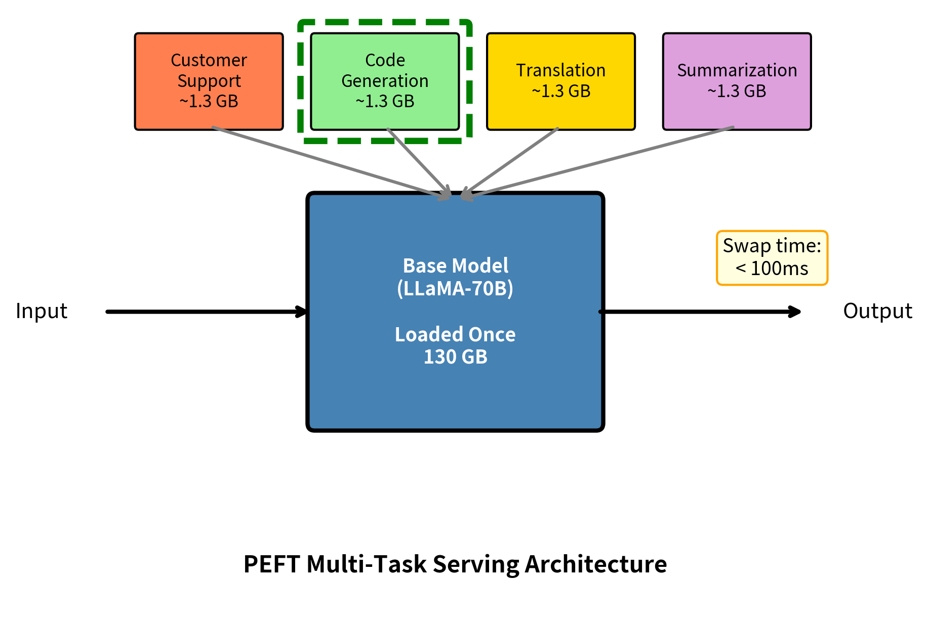
With adapter swapping, task switching takes milliseconds instead of 30-60 seconds required to reload full models. The base model occupies GPU memory once, and small adapters load nearly instantaneously. This architecture enables new deployment patterns: a single GPU can serve multiple applications by keeping adapters ready in system memory and swapping them into the active computation path as requests arrive. The result is better hardware utilization, lower costs, and faster response times for multi-task deployments.

PEFT's efficiency comes with trade-offs. Understanding when PEFT approaches full fine-tuning performance, and when it falls short, helps you choose the right approach for your application.

Research consistently shows PEFT achieves 90-99% of full fine-tuning performance across most tasks, with the gap depending on several factors:

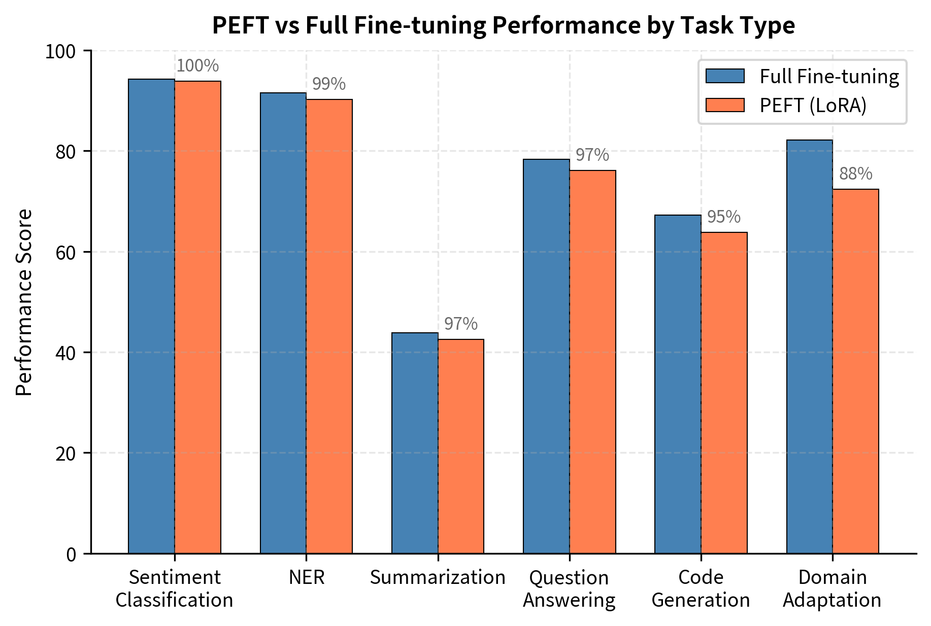
The data shows that PEFT performance closely trails full fine-tuning, with the gap remaining under 2% for simpler extraction tasks but widening for generative tasks.

PEFT performs best when the task primarily requires adapting the model's existing knowledge rather than learning fundamentally new capabilities:

Classification and extraction tasks like sentiment analysis, named entity recognition, and information extraction work exceptionally well with PEFT. These tasks leverage the model's pre-existing language understanding and primarily need to map representations to task-specific outputs. The performance gap versus full fine-tuning is typically less than 2%.

In-domain tasks where the target data distribution resembles the pre-training corpus see minimal degradation. If your task involves standard English text and common concepts, the base model's knowledge transfers directly with minor adaptation.

Limited training data scenarios can actually favor PEFT over full fine-tuning. With fewer trainable parameters, PEFT acts as implicit regularization, reducing overfitting risk on small datasets. As we discussed in Chapter 5 on fine-tuning data efficiency, the optimal parameter count depends on available training examples.

Certain scenarios reveal PEFT's limitations:

Domain shift presents the largest challenge. When adapting a model to specialized domains like legal, medical, or technical documentation with unique terminology and concepts, PEFT may underperform by 5-15%. The frozen base model lacks domain vocabulary and conceptual structures that full fine-tuning could develop. Domain adaptation, shown in the figure above, exhibits the largest performance gap.

Complex reasoning tasks that require restructuring the model's computation patterns show larger gaps. Tasks demanding multi-step reasoning or novel logical operations may need deeper modifications than small adapters provide. Code generation, which requires precise syntax and logical structure, typically shows larger PEFT gaps than text classification.

Very large datasets shift the economics. When you have millions of training examples and computational budget isn't constrained, full fine-tuning extracts more task-specific signal. PEFT's regularization effect becomes less beneficial when data is abundant.

Most PEFT methods have a "capacity" hyperparameter controlling how many additional parameters to train. For LoRA (covered in the next chapter), this is the rank $r$. The rank determines the dimensionality of the adapter's internal representation, with higher ranks enabling the adapter to capture more complex transformations but at the cost of additional parameters. Understanding this trade-off is essential for choosing appropriate PEFT configurations:

The figure reveals a characteristic pattern of diminishing returns as adapter capacity increases. Performance shows rapid initial improvement as rank increases from 1 to 8, then gains slow substantially. A rank of 8-32 typically captures most of the benefit while training only 0.08-0.32% of parameters. Higher ranks provide marginal gains at disproportionate parameter cost. This relationship suggests a natural "sweet spot" where the efficiency-performance trade-off is most favorable, though the exact location varies by task complexity.

When choosing between full fine-tuning and PEFT, consider these factors:

Multiple PEFT methods exist, each with different trade-offs. The upcoming chapters cover these techniques in detail:

• LoRA (Low-Rank Adaptation) adds trainable low-rank matrices to existing weight matrices. It's the most popular PEFT method, balancing simplicity, performance, and efficiency. We'll explore LoRA's mathematics and implementation in the next three chapters.

• QLoRA combines LoRA with quantization, enabling fine-tuning of 70B models on a single GPU by storing base weights in 4-bit precision.

• Prefix tuning and prompt tuning add trainable continuous vectors to the input, effectively learning soft prompts. These methods modify even fewer parameters than LoRA but may underperform on some tasks.

• Adapter layers insert small bottleneck modules between transformer layers. This was one of the first PEFT methods and remains effective, though LoRA has become more popular due to simpler integration.

Parameter-efficient fine-tuning addresses the practical challenges of adapting large language models to specific tasks. This chapter covered the motivations driving PEFT adoption:

• Storage costs multiply with tasks. Full fine-tuning requires storing a complete model copy per task. For LLaMA-70B with eight tasks, this means over 1 TB of weights. PEFT reduces this to approximately 130 GB by storing the base model once plus small adapters per task.

• Training memory limits accessibility. Full fine-tuning of LLaMA-70B requires 400+ GB of GPU memory for parameters, gradients, and optimizer states. PEFT reduces this by 3× by only computing gradients and optimizer states for the small trainable portion.

• Multi-task deployment benefits from adapter swapping. PEFT enables loading the base model once and swapping small adapters in milliseconds to switch tasks. This eliminates the 30-60 second latency of full model reloading.

• Performance trade-offs are task-dependent. PEFT achieves 90-99% of full fine-tuning performance for most tasks. Classification and extraction tasks see minimal gaps, while domain adaptation and complex reasoning show larger differences. The rank/capacity hyperparameter controls the trade-off between efficiency and performance.

• Start with PEFT for large models. Unless you have compelling evidence that full fine-tuning is necessary, PEFT provides an excellent efficiency-performance balance, especially for models above 7B parameters.

The following chapters dive into specific PEFT methods, starting with LoRA's elegant approach to low-rank weight updates.

Ready to test your understanding? Take this quick quiz to reinforce what you've learned about the motivations for parameter-efficient fine-tuning.