

Build mathematical models for random price movements. Learn simple random walks, Brownian motion properties, and Geometric Brownian Motion for asset pricing.
Choose your expertise level to adjust how many terms are explained. Beginners see more tooltips, experts see fewer to maintain reading flow. Hover over underlined terms for instant definitions.
Brownian Motion and Random Walk Models
The previous chapter documented the stylized facts of financial returns: fat tails, volatility clustering, and the approximate unpredictability of price movements. Now we turn to building mathematical models that capture at least the essence of these phenomena. The starting point, perhaps surprisingly, comes from 19th-century botany.
In 1827, Scottish botanist Robert Brown observed pollen grains suspended in water through a microscope. The particles moved erratically, jittering in seemingly random directions. This "Brownian motion" puzzled scientists until Einstein's 1905 paper explained it as the cumulative effect of countless molecular collisions, each individually invisible but collectively producing observable random movement.
Finance adopted this framework because stock prices exhibit similar behavior. Each trade, news item, or shift in sentiment acts like a molecular collision, nudging prices in unpredictable directions. The accumulated effect of millions of such nudges produces the irregular price paths we observe in markets.
This chapter builds Brownian motion from the ground up. We start with the simplest possible random process, a coin-flip walk on integers, then show how scaling this discrete model produces continuous Brownian motion in the limit. We then introduce Geometric Brownian Motion (GBM). This model adapts standard Brownian motion for asset prices, which cannot be negative and exhibit percentage returns. GBM forms the foundation for the Black-Scholes option pricing framework we'll develop in later chapters.
The Simple Random Walk
A random walk is exactly what it sounds like: a sequence of steps where each step's direction is determined by chance. The simplest version uses fair coin flips to decide whether to step up or down. Before diving into the formal mathematics, consider the intuition behind this construction. Imagine you are standing at the origin of a number line. You flip a fair coin repeatedly: if it lands heads, you take one step to the right; if tails, one step to the left. After many flips, where do you end up? This deceptively simple question reveals important properties of randomness and diffusive processes.
The random walk serves as our conceptual foundation because it distills randomness to its purest form. Each step is completely independent of every previous step, yet when we observe the accumulated position over time, patterns emerge. The walker tends to drift away from the origin, not because of any systematic force, but simply because random movements accumulate. This phenomenon, where independent random increments sum to produce gradually increasing uncertainty, lies at the heart of all diffusion processes in physics, biology, and finance.
A simple random walk is a discrete-time stochastic process where and:
where:
- : position of the random walk after steps
- : position after steps
- : independent step at time , taking values or with probability
- : current time step
The definition above encapsulates several important ideas. First, the recursive formulation tells us that the position at any time depends only on the previous position plus a new random increment. This is the Markov property in its simplest form: the future depends on the present but not on the past. Second, the alternative representation as a sum emphasizes that the current position is simply the cumulative total of all steps taken so far. This summation viewpoint connects directly to the Central Limit Theorem and explains why random walks eventually produce Gaussian distributions.
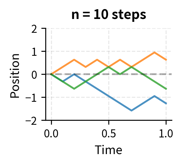
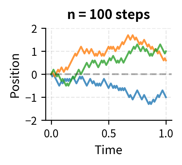
Starting at zero, after steps the walker's position is the sum of independent coin flips, each contributing (heads) or (tails). Let's simulate this process:
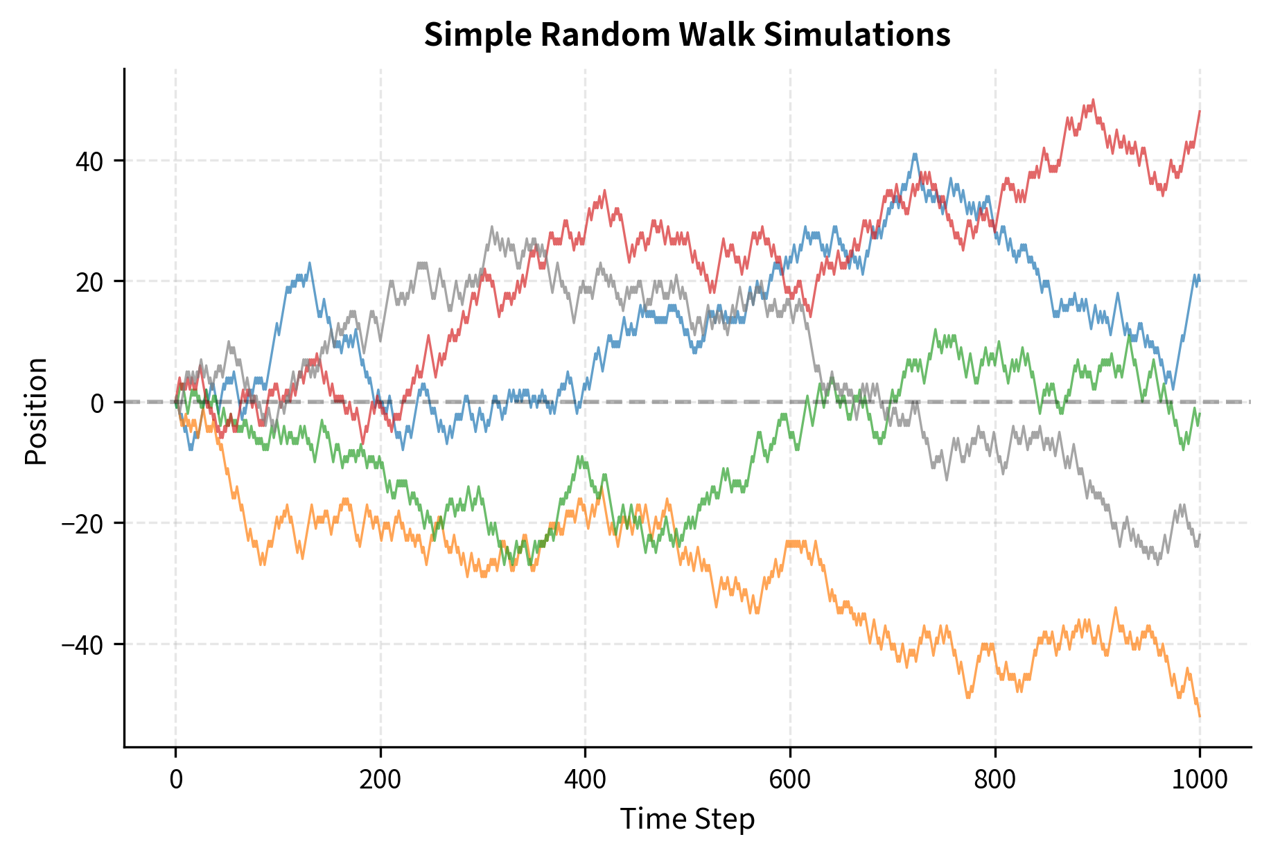
The paths exhibit several notable features. They wander away from zero but occasionally return. Some paths drift predominantly positive or negative over this sample, though with infinite time, a random walk returns to zero infinitely often (a property called recurrence). The paths look "rough" with jagged local movements but smoother trends at larger scales.
Properties of the Simple Random Walk
The mathematical properties of the simple random walk follow directly from the properties of sums of independent random variables, which we covered in the chapter on probability fundamentals. Understanding these properties builds the intuition we need for continuous-time models. Each property tells us something essential about how randomness accumulates over time.
Expected position: The first question we ask about any random process is: what is its average behavior? For a random walk, this amounts to asking where we expect the walker to be after steps. Since each individual step has an expected value of zero (heads contributes and tails contributes , each with probability , so ), and since expectation is linear, the expected position after steps must also be zero:
where:
- : expected value operator
- : position after steps
- : random step at index
This result, while mathematically straightforward, has a profound interpretation. The random walk has no systematic drift: on average, the walker stays at the origin. The coin is fair, so there is no bias pushing the walker in either direction. Yet this does not mean the walker stays near zero. As we shall see, the walker typically wanders quite far from the origin, even though the average position remains zero.
Variance of position: To understand how far the walker typically wanders, we need to compute the variance. Each step has variance . The variance equals one because the step is either or , so the squared step is always , and the squared mean is zero. Since the steps are independent, a fundamental property of variance tells us that the variance of a sum equals the sum of the variances:
where:
- : variance operator
- : position after steps
- : random step variable (variance is 1)
- : total number of steps
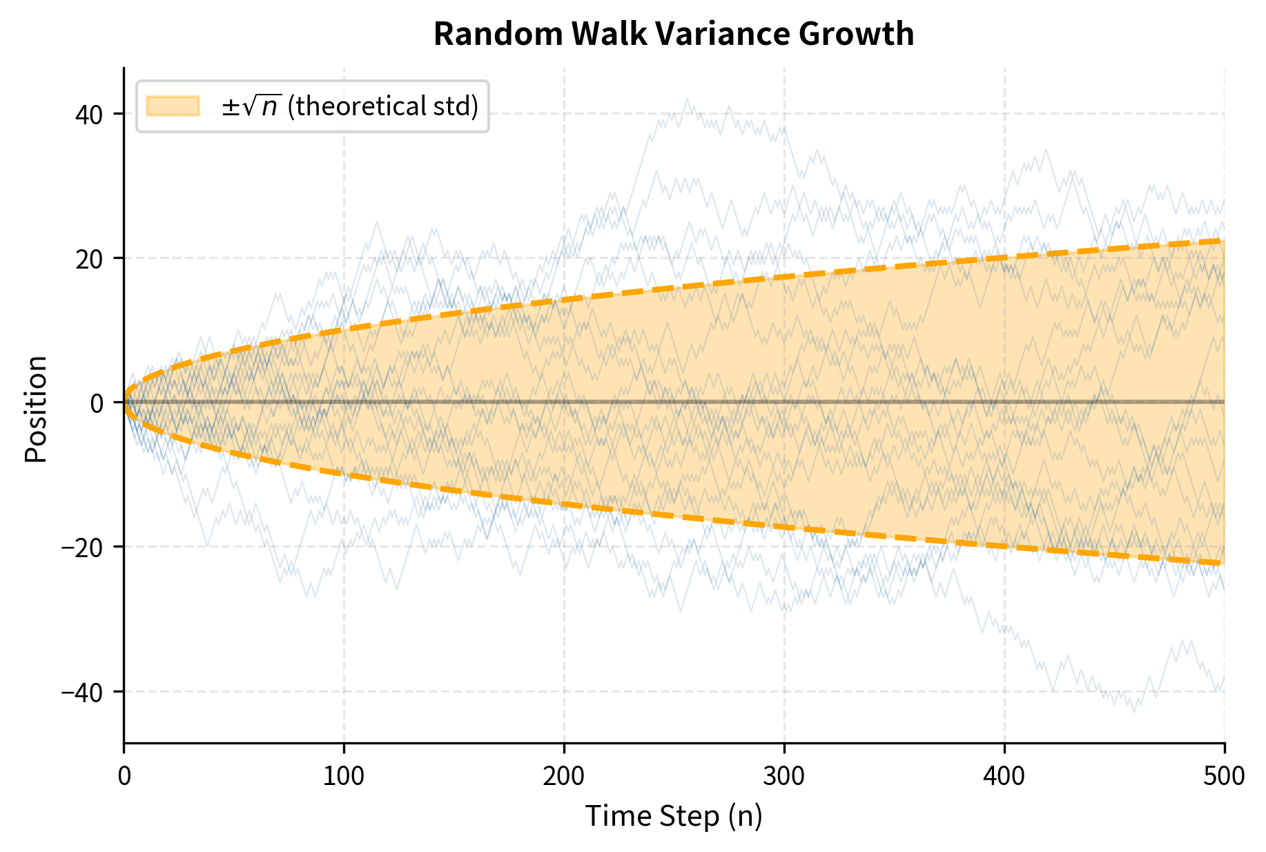
This reveals a fundamental insight: while the expected position stays at zero, the typical deviation from zero grows like . The standard deviation of the position is , meaning that after 100 steps, the walker is typically about 10 units away from the origin. After 10,000 steps, the typical distance grows to about 100 units. The walker doesn't systematically go anywhere, but uncertainty about its location increases over time. This square-root growth of uncertainty is a universal feature of diffusive processes, appearing in contexts ranging from heat conduction to portfolio theory.
Distribution of position: Beyond the mean and variance, we can characterize the entire probability distribution of the walker's position. By the Central Limit Theorem, for large , the sum of independent, identically distributed random variables approaches a normal distribution:
where:
- : position after steps
- : convergence in distribution
- : normal distribution with mean 0 and variance
The Central Limit Theorem is a fundamental result in probability theory. It tells us that regardless of the distribution of individual steps (as long as they have finite mean and variance), their sum becomes approximately Gaussian. For our random walk with steps, the convergence is rapid: even after just 30 or 40 steps, the distribution is nearly indistinguishable from a normal distribution. This explains why Gaussian distributions appear so frequently in nature and finance: whenever a quantity is the sum of many small independent contributions, normality emerges.
Let's verify these properties empirically:
The empirical mean is close to the theoretical value of zero, and the standard deviation matches the square root of the number of steps (10). This confirms the random walk's diffusive nature.
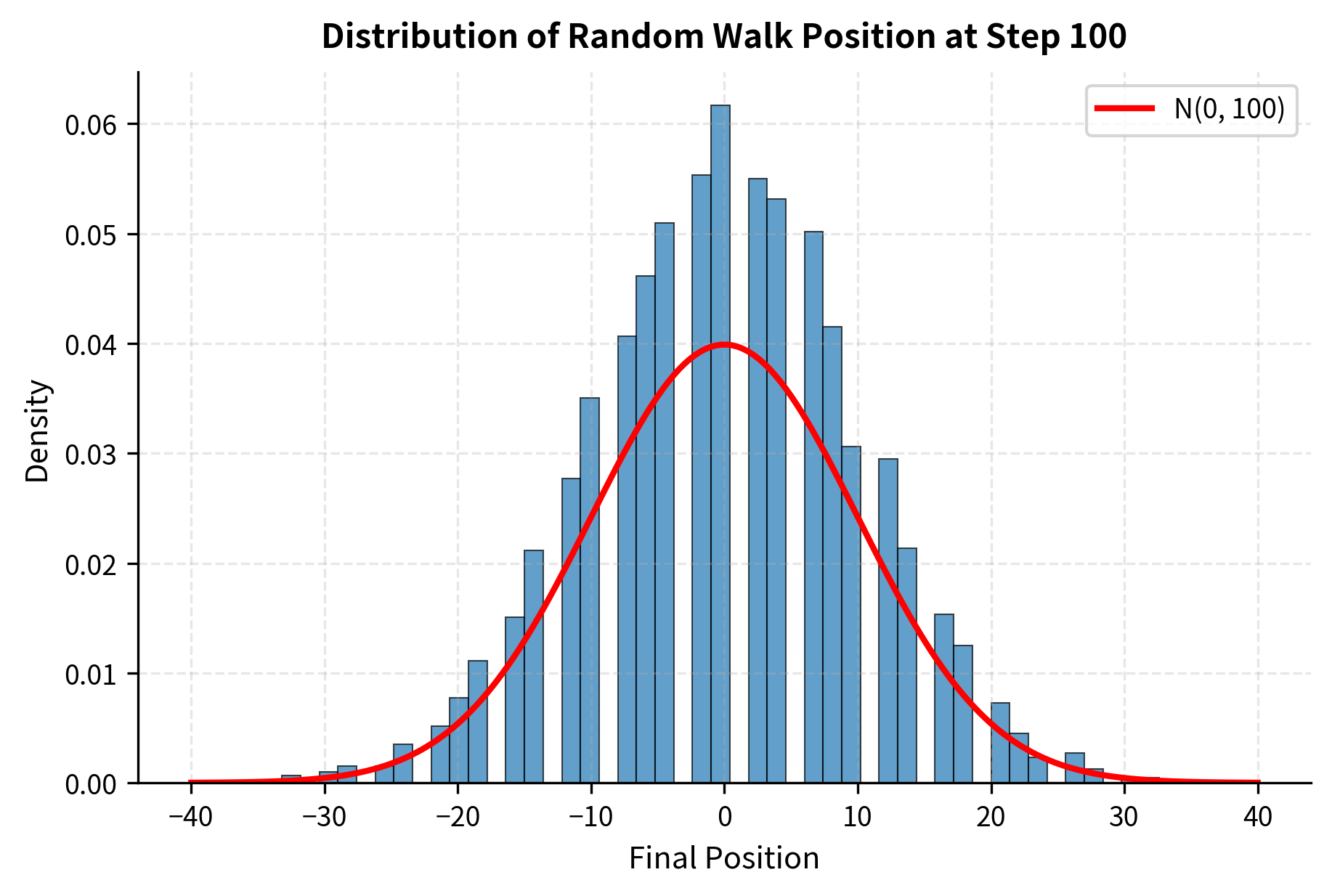
The empirical distribution matches the theoretical normal distribution well, confirming that the sum of many independent random steps produces Gaussian outcomes.
Independent Increments
A crucial property of random walks is that increments over non-overlapping time intervals are independent. This property is so fundamental that it becomes one of the defining characteristics of Brownian motion, and it has far-reaching implications for financial modeling. To understand what this means, consider two time intervals: from time to time , and from some earlier time to time (where ). The change in position from time to time is:
where:
- : position at time
- : position at time (where )
- : independent step at time
This increment depends only on steps , which are independent of all earlier steps . The steps in the future interval have nothing to do with the steps in the past interval because each coin flip is completely independent of all others. Therefore, knowing where the walker was at time tells you nothing about how far it will move between and .
This property has profound implications for financial modeling. If price changes follow a random walk, then past price movements cannot predict future movements: the process is a martingale with respect to its natural filtration. In practical terms, this means that technical analysis based on historical price patterns should not provide systematic profits if prices truly follow a random walk. The market incorporates all past information into the current price, and future price changes depend only on new information, which by definition cannot be predicted from the past.
From Discrete to Continuous: Scaling the Random Walk
Financial markets don't move in discrete integer steps. Prices change in small increments throughout the trading day, and we'd like a model that works in continuous time. The key insight is that if we make the random walk steps smaller and more frequent in the right proportion, the limiting process becomes a well-defined continuous-time object: Brownian motion. This passage from discrete to continuous is not merely a mathematical convenience but reflects the physical intuition that many small random shocks, occurring over short time intervals, aggregate into a smooth random process.
Consider a random walk where:
- Each step has size (instead of 1)
- Steps occur at time intervals of (instead of 1)
- We observe the process over a fixed time horizon
The number of steps in time is . As we let become smaller, the number of steps increases correspondingly. The position at time is the sum of all these steps:
where:
- : position at time
- : direction of step ()
- : size of each step
- : total number of steps ()
Now we face a crucial question: how should we scale as shrinks? If we keep fixed while , the variance of would grow without bound because we're adding more and more independent random variables. Conversely, if we shrink too quickly, the variance would go to zero and we'd be left with a deterministic process. The right scaling must preserve a finite, meaningful level of randomness.
The variance of this position is:
where:
- : variance of the position at time
- : number of steps
- : spatial step size
- : total time horizon
- : time interval between steps
For the variance to remain finite and proportional to as we take the limit , we need:
where:
- : spatial step size
- : time step size
- : variance scaling constant (volatility squared)
for some constant . This means .
This scaling relationship is the key to understanding why continuous-time models behave differently from ordinary calculus. As time steps shrink, the spatial steps shrink like the square root of time, not linearly. A step over time interval has magnitude proportional to , which is much larger than itself when is small. This creates paths that are continuous but have infinite length over any interval, and are nowhere differentiable. The square-root scaling is the mathematical signature of diffusion, and it underlies all the special rules of stochastic calculus that we'll develop in subsequent chapters.
Let's visualize this convergence:
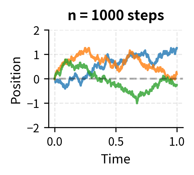
As we increase the number of steps, the paths become visually smoother. In the limit, we obtain Brownian motion: a continuous process that captures the essential randomness of the discrete walk.
Brownian Motion (Wiener Process)
Standard Brownian motion, also called a Wiener process (after mathematician Norbert Wiener who rigorously constructed it in the 1920s), is the continuous-time limit of the scaled random walk. It serves as the fundamental building block for stochastic calculus in finance. Just as the real numbers emerge as the completion of the rationals, Brownian motion emerges as the natural completion of discrete random walks when we demand continuity and the diffusive scaling property.
The existence of Brownian motion as a well-defined mathematical object is nontrivial. We are asking for a random process that has uncountably many time points, each with a random value, yet maintains consistency across all of them. Wiener's construction showed that such an object exists and is essentially unique, meaning that any process satisfying the defining properties must have the same distribution.
A stochastic process is a standard Brownian motion (or Wiener process) if:
-
(starts at origin)
-
has continuous sample paths (no jumps)
-
For , the increment is normally distributed with mean 0 and variance :
where:
- : value of Brownian motion at times and
- : normal distribution with variance
-
For non-overlapping intervals, increments are independent: if , then is independent of
These four properties completely characterize Brownian motion. Every process satisfying these axioms has the same probabilistic behavior, and these properties are sufficient to derive all other characteristics of the process. Let's unpack what each means:
Property 1 is simply a normalization. We can always shift a Brownian motion to start elsewhere, but the standard version starts at zero. This is analogous to how we define the standard normal distribution to have mean zero and variance one; we can always translate and scale as needed for specific applications.
Property 2 guarantees that sample paths are continuous functions of time. You can trace a Brownian path without lifting your pencil. This is essential for financial modeling since prices don't teleport. There are no jumps or gaps in a Brownian motion path. This continuity, combined with the other properties, creates paths that are continuous but extraordinarily irregular, as we shall see.
Property 3 tells us that the change in position over any time interval is Gaussian, with variance proportional to the length of the interval. The longer you wait, the more uncertain the position becomes, but uncertainty grows with the square root of time. A process that wanders for twice as long doesn't have twice the uncertainty; it has only times the uncertainty. This square-root law is fundamental and appears throughout finance, from portfolio volatility to option pricing.
Property 4 is the continuous-time version of the "no memory" property. Past movements don't help predict future movements. What happens between times and is completely independent of what happens between times and , as long as these intervals don't overlap. This is the continuous-time analog of independent coin flips in the discrete random walk.
Simulating Brownian Motion
To simulate Brownian motion numerically, we discretize time and generate increments from the appropriate normal distribution. Since we cannot actually compute with continuous time on a digital computer, we approximate Brownian motion by generating its values at a finite set of time points and connecting them. The key insight is that Property 3 tells us exactly what distribution to use for each increment.
If we divide into steps of size , each increment is:
where:
- : change in the process over step
- : value at time step
- : time step size ()
- : normal distribution with variance
We can write this as where are standard normal random variables. This representation is particularly useful for implementation because random number generators typically provide standard normal samples. We simply scale them by to obtain increments of the correct variance.
Key Properties of Brownian Motion
Beyond the defining properties, Brownian motion exhibits several remarkable characteristics that have important implications for financial modeling. These derived properties follow logically from the four axioms, but they provide additional insight into the nature of the process.
Stationary Increments: The distribution of depends only on the length of the interval, not on the starting time . This means the statistical behavior of the process is the same regardless of when you start observing it. Whether you look at the increment from time 0 to time 1 or from time 1000 to time 1001, the distribution is identical: in both cases. This stationarity reflects the idea that there is nothing special about any particular moment in time; the randomness is homogeneous across the entire timeline.
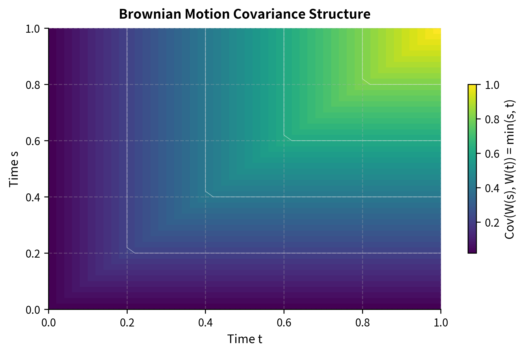
Gaussian Process: For any collection of times , the joint distribution of is multivariate normal. This is a powerful statement: not only is each individual normally distributed, but any finite-dimensional collection of values from the process is jointly Gaussian. The entire process is characterized by its mean function (identically zero) and its covariance function. The covariance between and is:
where:
- : covariance operator
- : Brownian motion values at times and
- : the smaller of the two time points
This formula has an intuitive interpretation. The covariance between and equals the length of time during which both have been "accumulating randomness" together. If , then and share the randomness from time 0 to time , which is exactly . After time , the additional randomness in is independent of , so it doesn't contribute to their covariance.
Markov Property: The future evolution of depends only on its current value, not on its past history. Formally, conditional on , the future increments are independent of . This "memoryless" property means that knowing the entire path up to time provides no more information about future behavior than knowing just the current value . The process forgets its history at every instant.
Martingale Property: Brownian motion is a martingale, meaning that the best forecast of the future value is the current value:
where:
- : expected value of given information at time
- : known value at current time
- : future time point
This follows because by the independence of increments. The increment is independent of all information available at time , and its unconditional expectation is zero. Therefore, the conditional expectation of given equals plus zero. The martingale property is central to financial theory because it captures the idea of a "fair game" where, on average, you neither gain nor lose.
Let's verify the covariance structure empirically:
The empirical covariance closely matches the theoretical value, confirming that the process correlation structure depends on the overlapping time duration.
Quadratic Variation
One of the most surprising and important properties of Brownian motion is its quadratic variation. This property is what makes stochastic calculus fundamentally different from ordinary calculus, and understanding it is essential for deriving results like Itô's lemma and the Black-Scholes equation.
For any ordinary smooth function , such as a polynomial or a sine wave, the sum of squared increments goes to zero as the partition becomes finer:
where:
- : a differentiable (smooth) function
- : time points in the partition
- : number of intervals in the partition
The intuition is straightforward: for a smooth function, each increment is approximately , so the squared increment is approximately . Summing such terms gives order , which goes to zero as .
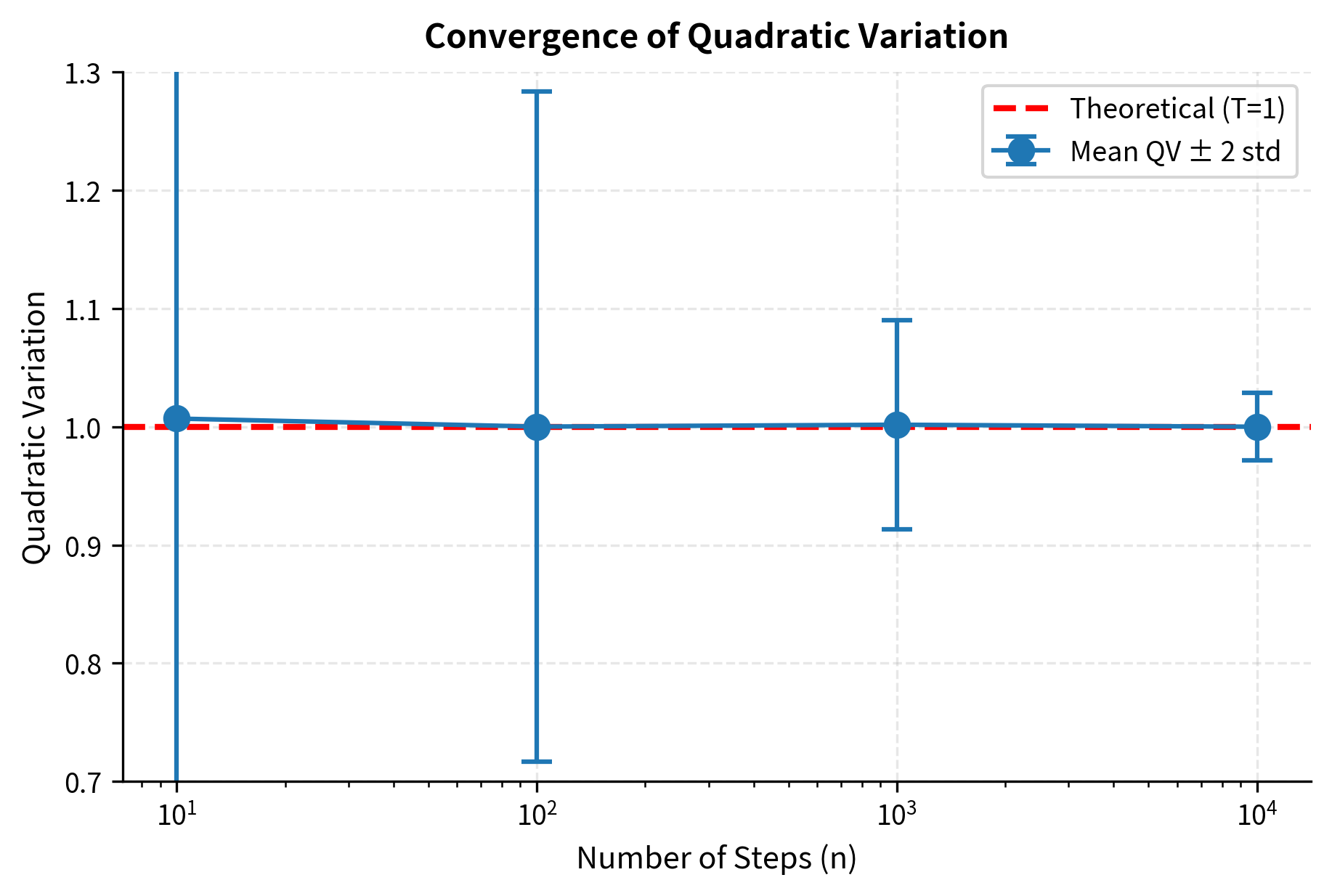
For Brownian motion, something entirely different happens. The quadratic variation over converges to :
where:
- : Brownian motion value at time
- : total length of the time interval
- : number of steps
This is often written in differential form as , a shorthand that captures the essential relationship.
The intuition is that while each increment is small (of order ), there are of them. When we square the increments, each contributes order , and summing terms gives order . More precisely, each has expected value , and by a law of large numbers argument, the sum converges to its expected value as the number of terms grows.
This non-zero quadratic variation is why stochastic calculus differs from ordinary calculus and leads to Itô's lemma, which we'll develop in the next chapter. When we apply the chain rule to a function of Brownian motion, we cannot ignore the second-order terms because the quadratic variation contributes at the same order as the first-order terms. This is the mathematical origin of the mysterious correction that appears in option pricing formulas.
As the number of steps increases, the quadratic variation converges to with decreasing variance. This deterministic limit of a random quantity is a remarkable feature of Brownian motion.
Nowhere Differentiability
Brownian motion paths are continuous everywhere but differentiable nowhere. This seems paradoxical since continuity usually suggests some smoothness, but Brownian paths are maximally irregular. They are continuous because small changes in time produce small changes in position (no jumps), yet they are so jagged that no tangent line exists at any point.
The intuition comes from the scaling property. Over a small time interval , the typical change in position is of order , not . The "derivative" would be:
where:
- : value of Brownian motion at time
- : small time increment
- : indicates the order of magnitude
As , this ratio blows up rather than converging. The path oscillates too wildly at every scale for a derivative to exist. If you zoom in on any portion of a Brownian path, you don't see a straight line approximating the curve; instead, you see the same jagged, irregular behavior at the finer scale. This self-similarity at all scales is a hallmark of fractal geometry, and Brownian motion is indeed a fractal object with Hausdorff dimension 1.5.
This has practical implications: we cannot write as an ordinary derivative. Instead, we work with the differential itself, leading to stochastic differential equations rather than ordinary ones. The notation does not mean an infinitesimal change divided by an infinitesimal time; it is a fundamentally different mathematical object that requires new rules for manipulation.
![Full Brownian motion path over the interval [0, 1]. The trajectory exhibits characteristic roughness and irregularity.](https://cnassets.uk/notebooks/2_brownian_motion_random_walk_files/brownian-motion-self-similarity-full.png)
![A 10x zoom of the same path over [0.4, 0.5]. The local structure resembles the global path, illustrating self-similarity.](https://cnassets.uk/notebooks/2_brownian_motion_random_walk_files/brownian-motion-self-similarity-zoom10.png)
![A 100x zoom over [0.44, 0.45]. The fractal nature is evident as the path remains non-differentiable even at fine scales.](https://cnassets.uk/notebooks/2_brownian_motion_random_walk_files/brownian-motion-self-similarity-zoom100.png)
Geometric Brownian Motion
Standard Brownian motion can go negative, which makes it unsuitable for modeling asset prices directly. A stock price of negative $50 is meaningless. We need a modification that ensures prices stay positive and captures the multiplicative nature of returns, where a 10% gain followed by a 10% loss doesn't return you to the starting point. If you start with $100, gain 10% to reach $110, then lose 10%, you end at $99, not $100.
Geometric Brownian Motion (GBM) solves both problems by modeling the logarithm of the price as Brownian motion with drift. By taking the exponential of a process that can range from negative infinity to positive infinity, we obtain a process that ranges from zero to positive infinity, which is exactly the domain of asset prices. The multiplicative structure of percentage returns emerges naturally from this construction.
A stochastic process follows Geometric Brownian Motion if it satisfies the stochastic differential equation:
where:
- : asset price at time
- : drift rate (expected return)
- : volatility (standard deviation of returns)
- : standard Brownian motion
Equivalently, follows Brownian motion with drift.
The stochastic differential equation above deserves careful interpretation. The term represents the deterministic drift: if there were no randomness, the price would grow exponentially at rate . The term represents the random fluctuations: the price is continuously perturbed by Brownian shocks, with the magnitude of these shocks proportional to the current price level. This proportionality is crucial because it means that a $100 stock and a $1000 stock experiencing the same percentage volatility will have different dollar volatilities.
The solution to this SDE is:
where:
- : asset price at time
- : initial asset price
- : drift parameter
- : volatility parameter
- : value of Brownian motion at time
We'll derive this solution rigorously using Itô's lemma in the next chapter. For now, let's understand why this form makes sense and explore its properties.
Why the Drift Adjustment?
You might expect the exponent to simply be , but there's an additional term. This correction arises from the convexity of the exponential function and the non-zero quadratic variation of Brownian motion. It is perhaps the most important example of how stochastic calculus differs from ordinary calculus.
Consider the logarithm of the price process:
where:
- : log-price at time
- : price at time
- : drift of the log-price process
- : standard Brownian motion source of noise
This is an arithmetic Brownian motion with drift and volatility . The term is sometimes called the "Itô correction" or "convexity adjustment."
The drift represents the expected instantaneous return , but because of Jensen's inequality, the expected log return is lower:
where:
- : expected value operator
- : return ratio over time
- : arithmetic drift rate
- : convexity adjustment
To understand this intuitively, consider what happens to the average of $100 invested in two equally likely scenarios: either the price doubles to $200 or it halves to $50. The arithmetic average outcome is (200 + 50)/2 = $125, representing a 25% gain. But the geometric average (or equivalently, the average of log returns) is = $100, representing a 0% gain. The arithmetic mean exceeds the geometric mean whenever there is volatility, and the gap is approximately .
For typical equity parameters (, ), the difference is or 2% per year, which is economically significant. If you earn an expected arithmetic return of 10% per year, you actually experience expected log returns of only 8% per year. Over long horizons, this difference compounds substantially.
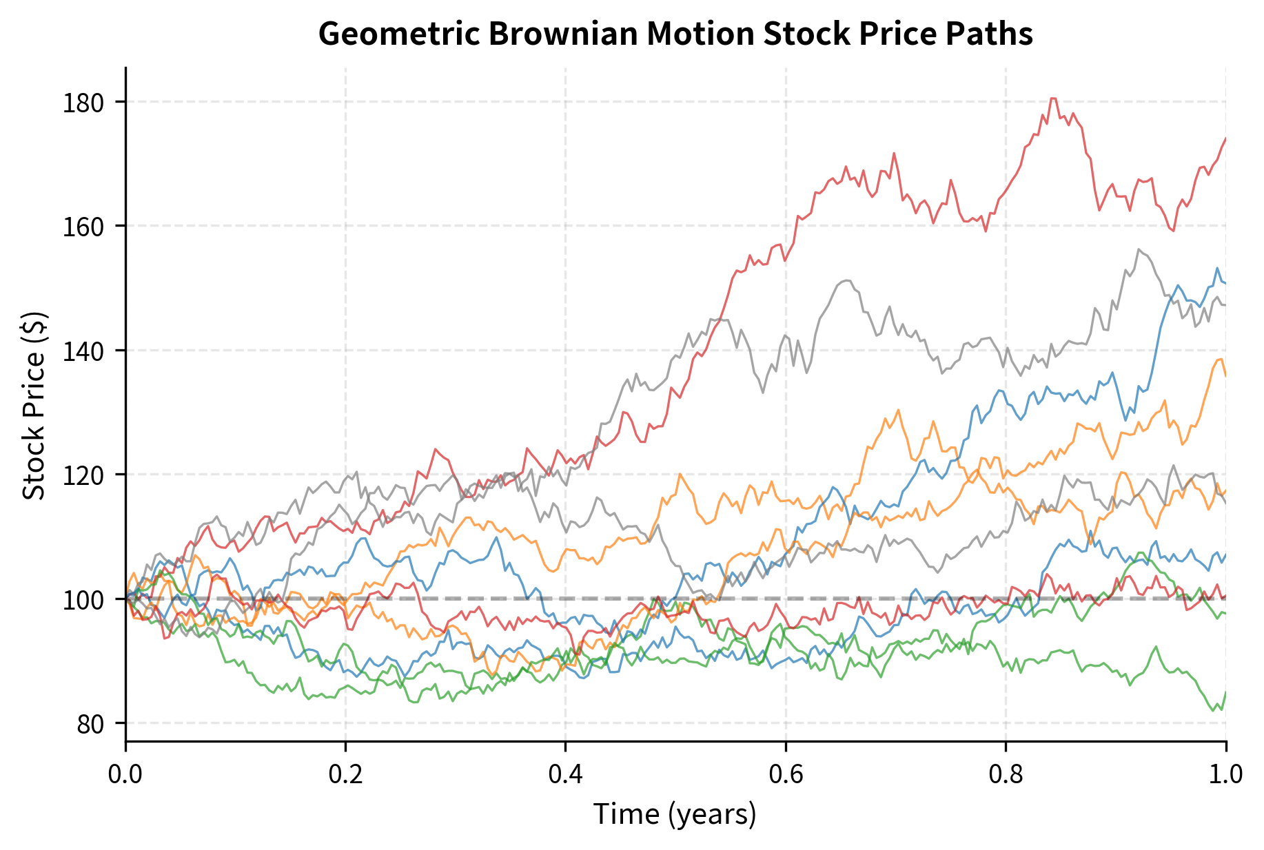
Simulating GBM
We can simulate GBM in two equivalent ways: directly using the exact solution, or by discretizing the SDE.
Exact simulation: Since we have a closed-form solution, we can generate directly:
where:
- : simulated price at time
- : starting price
- : drift and volatility parameters
- : Brownian motion realization
This approach is highly efficient because we only need to simulate the Brownian motion once, then apply the exponential transformation. There is no discretization error because we are using the exact solution at each time point.
Euler discretization: Approximate the SDE over small time steps:
where:
- : price at the next time step
- : current price
- : drift rate
- : volatility
- : time increment
- : standard normal random variable
The Euler method approximates the continuous SDE by treating the drift and diffusion terms as constant over each small time step. This introduces discretization error that shrinks as , but for any finite time step, the approximation is not exact.
The exact method is preferable when possible since it avoids discretization error.
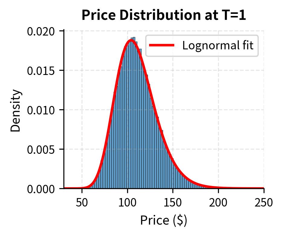
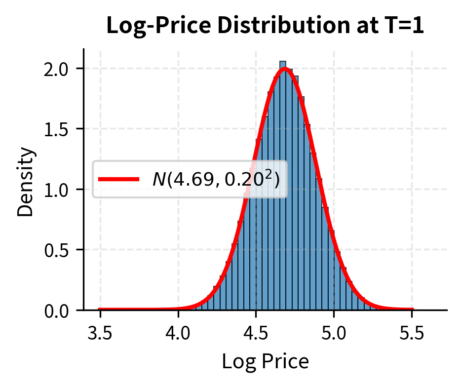
Lognormal Distribution of Prices
Since is normally distributed, itself follows a lognormal distribution. This is a direct consequence of the GBM solution: the exponential of a normal random variable is lognormal. Specifically:
where:
- : natural logarithm of price at time
- : normal distribution notation
- : initial price
- : drift rate
- : volatility
- : time elapsed
- : mean of the log-price
- : variance of the log-price
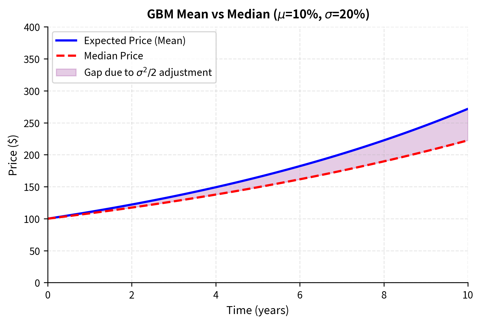
From this, we can derive several important quantities:
- Expected price:
- Variance of price:
- Median price:
The mean exceeds the median because the lognormal distribution is right-skewed. There's a small probability of very large price increases, which pulls the mean above the median. This skewness increases with volatility and time, reflecting the asymmetry between percentage gains and losses: a stock can gain 100% or 200%, but it can only lose at most 100%.
Let's verify the distribution:
The simulation results confirm that while the log-prices are normally distributed, the prices themselves are lognormally distributed. The mean price exceeds the median, reflecting the positive skewness of the lognormal distribution.
Returns Under GBM
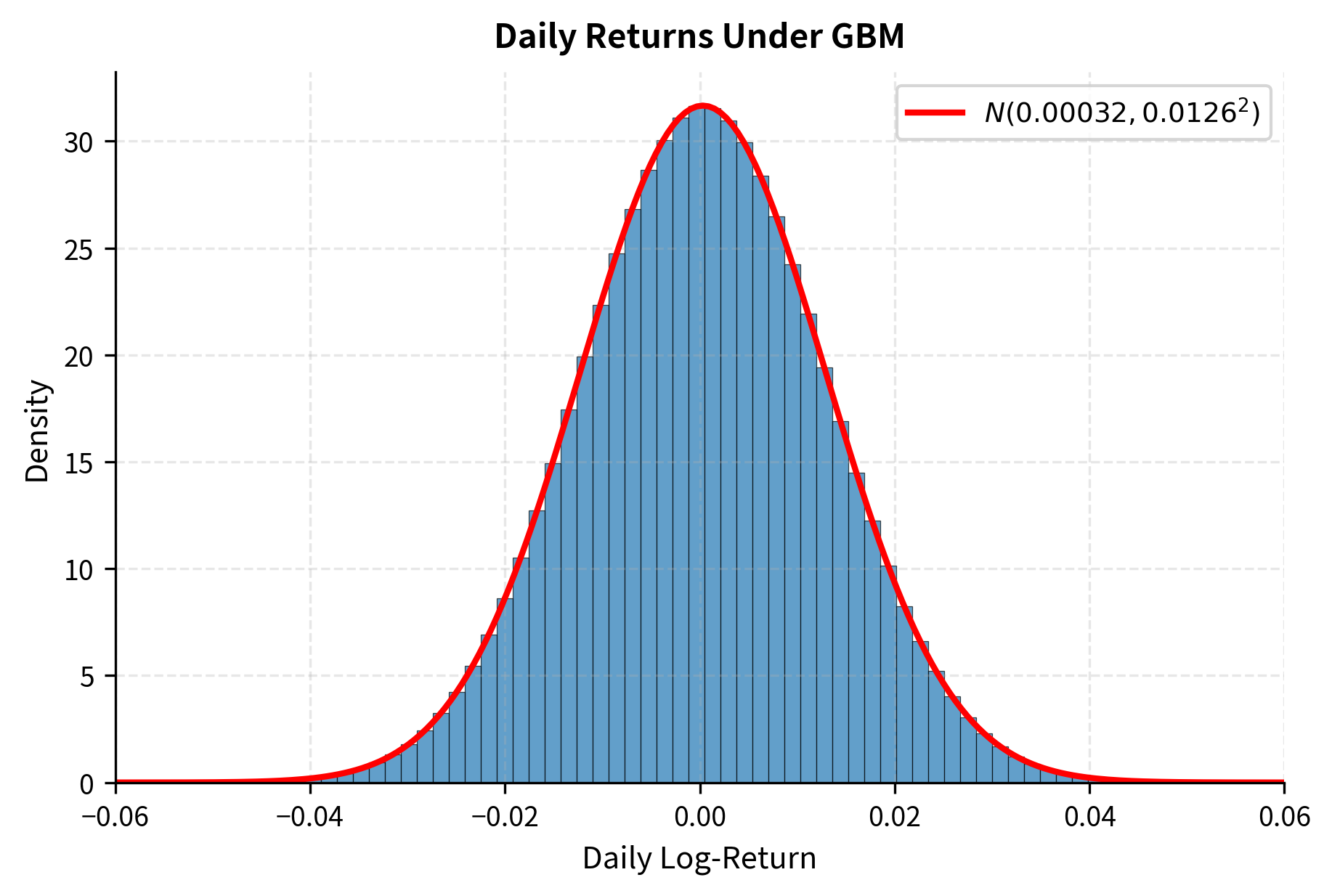
Under GBM, the log-return over period is:
where:
- : log-return over the interval
- : price ratio
- : length of the time interval
- : Brownian increment over the interval
Since the Brownian increment is normally distributed with mean zero and variance , the log-return is normally distributed with mean and variance . This matches one of the stylized facts we discussed in the previous chapter: returns are approximately symmetric and close to normal for moderate return magnitudes.
For small , the simple return approximates the log-return:
where:
- : simple percentage return
- : logarithmic return
This approximation follows from the Taylor expansion for small . When the percentage return is small (say, under 10%), the difference between simple and log returns is negligible for most practical purposes.
The moments of the simulated log-returns match the theoretical values for a normal distribution: mean close to zero, standard deviation consistent with volatility, and negligible skewness and excess kurtosis.
Connecting GBM to Real Market Data
How well does GBM describe actual stock prices? Let's compare simulated GBM paths against real market behavior using the stylized facts from the previous chapter.
We'll calibrate GBM parameters from historical data and examine where the model succeeds and fails.
The parameter estimation works well when data truly comes from GBM. But real markets deviate from GBM assumptions in systematic ways.
Key Parameters
The key parameters for the Geometric Brownian Motion model are:
- : Initial asset price. The starting point for the simulation or pricing path.
- μ: Drift rate (expected return). Represents the annualized average growth rate of the asset.
- σ: Volatility. The standard deviation of the asset's logarithmic returns, measuring uncertainty.
- T: Time horizon. The total duration for which the price path is simulated.
- dt: Time step size. Smaller steps () lead to more accurate approximations of the continuous process.
Limitations and Impact
Geometric Brownian Motion has been highly influential in quantitative finance, forming the foundation for the Black-Scholes option pricing framework. Yet its limitations are equally important to understand.
GBM assumes returns are normally distributed with constant volatility, but as we documented in the chapter on stylized facts, real returns exhibit fat tails and volatility clustering. Extreme market movements like the 1987 crash or the 2008 financial crisis are orders of magnitude more likely than GBM predicts. A daily return of is essentially impossible under GBM with typical parameters ( would make this a 25-standard-deviation event), yet such moves do occur. This misspecification matters enormously for risk management and option pricing, particularly for out-of-the-money options where the probability of extreme moves determines value.
The assumption of constant volatility is equally problematic. Real volatility varies over time and tends to cluster: periods of high volatility are followed by more high volatility. The VIX index, which measures implied volatility in S&P 500 options, swings from below 10 in calm markets to above 80 during crises. GBM has no mechanism to capture this variation. Models like GARCH (which we'll explore in later chapters on time series) and stochastic volatility models address this limitation by allowing volatility itself to evolve randomly.
GBM also assumes prices are continuous with no jumps. In reality, prices can gap overnight on earnings announcements or news events. Jump-diffusion models extend GBM by adding occasional discontinuous moves, better matching the observed behavior of individual stocks around events.
Despite these limitations, GBM remains foundational for several reasons. First, it provides closed-form solutions that build intuition. The Black-Scholes formula, which we'll derive in upcoming chapters, shows exactly how option prices depend on underlying price, volatility, and time. This transparency is invaluable for understanding risk sensitivities. Second, GBM is mathematically tractable and serves as a building block for more complex models. Once you understand GBM, you can add stochastic volatility, jumps, or other features to create more realistic models. Third, for many applications, GBM is "good enough." For at-the-money options with short maturities, GBM pricing errors are often within bid-ask spreads. The model's simplicity makes it practical for real-time trading applications where computational speed matters.
The practical lesson is to use GBM as a starting point, not an endpoint. Understand its assumptions, recognize when they fail, and know how to extend the framework when higher accuracy is needed. The options chapter on implied volatility and volatility smiles will show how practitioners implicitly correct for GBM's limitations through the prices they quote.
Summary
This chapter built the mathematical foundation for modeling random price movements in continuous time:
Random walks provide an intuitive starting point. A simple random walk adds independent steps, producing positions with zero mean and variance proportional to time. The Central Limit Theorem ensures that the distribution approaches normal as the number of steps grows.
Brownian motion emerges as the continuous-time limit of appropriately scaled random walks. It is characterized by four properties: starting at zero, continuous paths, normally distributed increments with variance proportional to time, and independence of increments over non-overlapping intervals. The quadratic variation of Brownian motion equals elapsed time rather than zero, a property that underlies all of stochastic calculus.
Geometric Brownian Motion adapts Brownian motion for asset prices by modeling log-prices rather than prices. This ensures prices remain positive and captures the multiplicative nature of returns. Under GBM, prices follow a lognormal distribution and log-returns are normally distributed with constant volatility.
These models provide the mathematical foundation for option pricing theory. In the next chapter, we'll develop Itô's lemma, which tells us how functions of Brownian motion evolve and allows us to derive the Black-Scholes equation for option prices.
Quiz
Ready to test your understanding? Take this quick quiz to reinforce what you've learned about Brownian motion and random walk models.

Comments