

Derive the Black-Scholes-Merton PDE using Itô's lemma, delta hedging, and no-arbitrage principles. Complete step-by-step mathematical derivation.
Choose your expertise level to adjust how many terms are explained. Beginners see more tooltips, experts see fewer to maintain reading flow. Hover over underlined terms for instant definitions.
Derivation of the Black-Scholes-Merton PDE
The Black-Scholes-Merton partial differential equation stands as one of the most important results in mathematical finance. Published in 1973 by Fischer Black, Myron Scholes, and Robert Merton, this equation provides a framework for pricing derivative securities by showing that the price of any derivative must satisfy a specific PDE under certain assumptions. What makes this result remarkable is that the equation contains no reference to investor preferences or expected returns: the derivative price depends only on observable quantities and the assumption of no arbitrage.
In this chapter, you will learn how to derive this PDE from first principles using the tools we've developed in previous chapters. The derivation follows a beautiful logical chain: we assume stock prices follow geometric Brownian motion, apply Itô's lemma to find the dynamics of a derivative's price, construct a portfolio that eliminates all randomness through dynamic hedging, and invoke the no-arbitrage principle to obtain the final equation. Understanding this derivation deeply prepares you for the practical applications covered in subsequent chapters, where we'll solve the PDE to obtain explicit pricing formulas.
The Model Assumptions
Before deriving the PDE, we must clearly state the assumptions underlying the Black-Scholes-Merton framework. These assumptions define an idealized market that, while not perfectly realistic, captures enough structure to produce useful results. Each assumption plays a specific role in the derivation, and understanding why each is needed helps you appreciate both the power and the limitations of the resulting framework.
The complete set of assumptions required for the BSM framework:
- The stock price follows geometric Brownian motion with constant drift and volatility
- Trading occurs continuously with no transaction costs
- Short selling is permitted without restrictions
- There are no arbitrage opportunities
- Securities are infinitely divisible
- A risk-free asset exists with constant interest rate
- The stock pays no dividends during the option's life
- Markets are frictionless with no taxes or bid-ask spreads
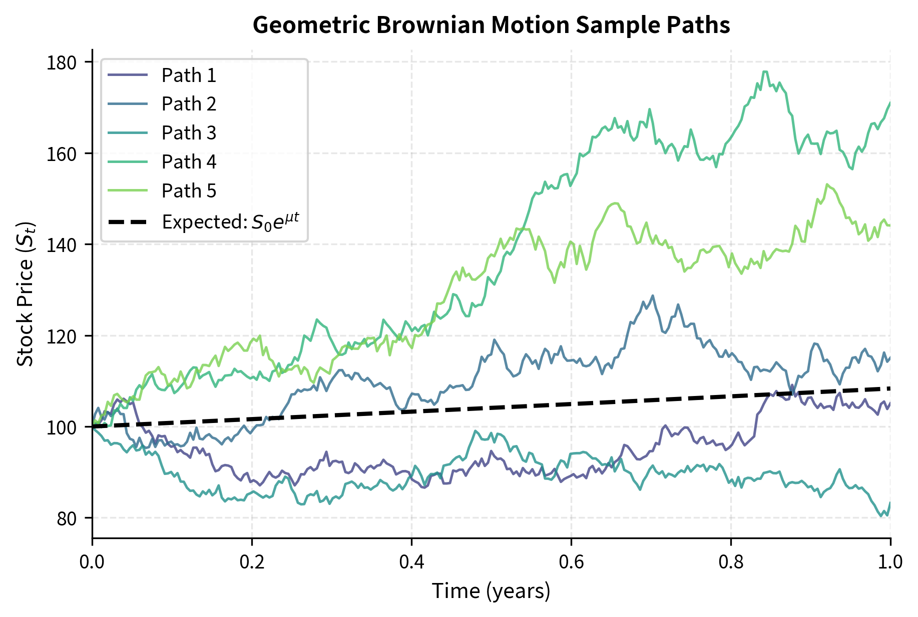
The most critical assumption is that the stock price follows geometric Brownian motion. This mathematical model captures the essential features we observe in real stock prices: they fluctuate randomly, they exhibit larger absolute movements when prices are higher, and they cannot become negative. The geometric Brownian motion specification takes the form:
where:
- : stock price at time
- : expected return (drift) of the stock
- : volatility of stock returns
- : increment of a standard Wiener process (random shock)
- : small time increment
To understand this equation intuitively, think of the stock price as experiencing two simultaneous influences over each infinitesimally small time interval. The first influence, captured by , represents the deterministic drift: on average, the stock price tends to grow at rate . This drift is proportional to the current price, reflecting the multiplicative nature of returns. The second influence, captured by , represents the random shocks that buffet the price. The Wiener increment is the mathematical formalization of "white noise," introducing unpredictable fluctuations. The volatility parameter scales these fluctuations, and multiplying by ensures that absolute price movements scale with the price level.
As we discussed in our chapter on Brownian Motion and Random Walk Models, this model ensures stock prices remain positive and that returns are normally distributed. The positivity follows from the multiplicative structure: since we're multiplying by , the process never crosses zero.
Let denote the price of a derivative security that depends on the stock price and time . Our goal is to determine what equation must satisfy. We make no assumptions about the specific form of : it could represent a call option, a put option, or any other derivative whose payoff depends on the stock price at maturity. This generality is one of the beautiful features of the BSM framework: rather than deriving separate formulas for each type of derivative, we derive a single equation that all derivatives must satisfy.
Dynamics of the Derivative Price
To find how the derivative price changes over time, we must apply Itô's lemma. This is where the machinery of stochastic calculus becomes essential. In ordinary calculus, if you have a function and changes by a small amount , then changes by approximately . But in stochastic calculus, the presence of random fluctuations introduces additional terms that have no analog in the deterministic world.
Recall from our chapter on Itô's Lemma and Stochastic Calculus that for any sufficiently smooth function where follows a diffusion process, the differential has a specific form that accounts for the second-order effects of stochastic calculus. The key insight is that terms involving , which would vanish in ordinary calculus because they're second-order small, actually contribute to first order in stochastic calculus because .
Since follows geometric Brownian motion, Itô's lemma gives:
where:
- : price of the derivative security
- : sensitivity of option value to time (Theta)
- : sensitivity of option value to stock price (Delta)
- : curvature of option value with respect to stock price (Gamma)
- : small time increment
- : change in stock price
Notice that this formula looks almost like the ordinary chain rule, with one crucial addition: the final term involving the second derivative. This term arises specifically because of the stochastic nature of the price process. In deterministic calculus, this term would be negligibly small, a second-order effect effect that vanishes in the limit. But in stochastic calculus, the roughness of Brownian motion paths means this term survives and contributes meaningfully to the dynamics.
We need to evaluate by substituting the expression for and applying Itô multiplication rules. This calculation reveals why stochastic calculus differs fundamentally from ordinary calculus:
where:
- : change in stock price
- : drift coefficient
- : volatility coefficient
- : stock price
- : small time increment
- : Wiener process increment
The Itô multiplication rules deserve careful attention because they encode the essence of what makes stochastic calculus different. The rule is intuitive: when we square an infinitesimally small quantity, we get something even more negligibly small. The rule follows from similar reasoning. But the rule is remarkable: squaring a random increment of order produces something of order , which is not negligible. This is the mathematical expression of the fact that Brownian motion paths are extremely rough, changing direction infinitely often in any finite time interval.
Substituting and back into the expression for and grouping terms, we arrive at the complete dynamics of the derivative price:
where:
- : change in the derivative price
- : price of the derivative
- : stock price
- : time
- : expected return of the stock
- : volatility of the stock
- : standard Wiener process increment
This equation tells us that the derivative price has both a deterministic component (the term) and a random component (the term). The deterministic component captures the systematic evolution of the derivative price due to the passage of time, the drift in the stock price, and the convexity effect from the second derivative. The random component, proportional to , represents the uncertainty in the derivative price arising from the uncertainty in the stock price.
The presence of means that holding the derivative alone exposes you to the same source of randomness as holding the stock. Both the stock and the derivative are driven by the same Brownian motion, though with different sensitivities. This observation is the crucial starting point for the hedging argument that follows.
Constructing the Hedged Portfolio
The key insight of Black and Scholes was that you can construct a portfolio combining the derivative and the stock that eliminates all randomness. This is the essence of delta hedging: by holding the right proportion of stock against the derivative, you create a riskless portfolio. The possibility of such elimination arises because both the stock and the derivative are driven by the same source of randomness, namely the Wiener process . If we can find the right mix, the random fluctuations in one position will exactly offset the random fluctuations in the other.
Consider a portfolio consisting of:
- Long one derivative (value )
- Short shares of stock (value )
The word "short" here means we have sold shares we don't own, creating a negative position in the stock. This is a standard operation in financial markets, and one of our model assumptions permits it without restriction. The portfolio value is:
where:
- : value of the hedged portfolio
- : value of the derivative
- : number of shares of stock held short
- : current stock price
The change in portfolio value over a small time interval captures how the portfolio responds to all the forces acting on its components:
where:
- : change in portfolio value
- : change in derivative value
- : number of shares held short
- : change in stock price
This expression reflects the fact that when we're short shares, we lose money when the stock price rises and gain money when it falls. The negative sign captures this inverse relationship.
Substituting our expressions for and , we obtain a detailed view of all the terms affecting the portfolio:
where:
- : change in portfolio value
- : value of the derivative
- : stock price
- : number of shares held short
- : expected return of the stock
- : volatility of the stock
- : small time increment
- : Wiener process increment
Now we rearrange this expression by collecting the and terms separately. This organizational step reveals the structure of the portfolio's dynamics:
where:
- : change in portfolio value
- : value of the derivative
- : stock price
- : number of shares held short
- : expected return of the stock
- : volatility of the stock
- : small time increment
- : Wiener process increment
The coefficient of represents the portfolio's exposure to randomness. If this coefficient is nonzero, the portfolio value fluctuates randomly. If we can make this coefficient vanish, the portfolio becomes deterministic over the next instant.
To eliminate the random component, we choose such that the coefficient of equals zero:
where:
- : number of shares to short
- : derivative's delta
The solution is elegantly simple: we should hold exactly shares short for each unit of derivative we hold long. This quantity, the partial derivative of the option price with respect to the stock price, measures how sensitive the option is to stock price movements. It tells us exactly how many shares we need to offset that sensitivity.
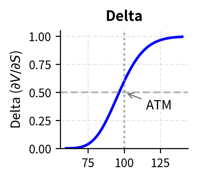
The quantity is called the delta of the derivative. It represents the sensitivity of the derivative price to changes in the underlying stock price, and it equals the number of shares needed to hedge one unit of the derivative. For a call option, delta typically ranges between 0 and 1, indicating that the option price moves less than dollar-for-dollar with the stock. For a put option, delta ranges between -1 and 0.
With this choice of , something remarkable happens. Not only does the random term vanish, but the terms involving also cancel out. Let us trace through this simplification carefully:
where:
- : change in value of the hedged portfolio
- : price of the derivative
- : stock price
- : volatility
- : time
- : small time increment
This This is a remarkable result: the portfolio's change has no random component. The portfolio is instantaneously riskless. Furthermore, the expected return of the stock has completely vanished from the expression. The portfolio change depends only on the passage of time, the volatility, and the Greeks of the derivative. This disappearance of is profound: it means the derivative price will not depend on how optimistic or pessimistic investors are about the stock's future direction.
Applying the No-Arbitrage Principle
We now have a portfolio with no risk over the next instant. Building on the no-arbitrage principle from our previous chapter on risk-neutral valuation, a riskless portfolio must earn the risk-free rate. The logic is ironclad: if the portfolio earned more than the risk-free rate, you could borrow money at the risk-free rate, invest in the portfolio, and pocket the difference as guaranteed profit. If it earned less, you could short the portfolio, invest the proceeds in the risk-free asset, and again earn guaranteed profit. Either scenario represents arbitrage, a free lunch that cannot persist in a well-functioning market.
The no-arbitrage condition states:
where:
- : risk-free interest rate
- : value of the riskless portfolio
- : time increment
This equation simply says that the return on a riskless investment must equal the risk-free rate. The risk-free rate represents the return you could earn on a perfectly safe investment, such as a government bond or a bank deposit.
Now we substitute our expressions for and and perform algebraic manipulations to extract the PDE:
where:
- : derivative price
- : time
- : stock price
- : risk-free rate
- : volatility
This is the Black-Scholes-Merton partial differential equation. We have arrived at a fundamental constraint that any arbitrage-free derivative price must satisfy. The equation emerged from combining three key ingredients: the assumption that stock prices follow geometric Brownian motion, the application of Itô's lemma to characterize derivative dynamics, and the no-arbitrage condition that riskless portfolios must earn the risk-free rate.
The Black-Scholes-Merton PDE
Any derivative security whose value depends on a stock following geometric Brownian motion must satisfy:
where:
- : price of the derivative security
- : current stock price
- : risk-free interest rate
- : volatility of the underlying stock
This equation has several notable features worth examining carefully, as they reveal deep insights about derivative pricing.
The drift does not appear. The expected return on the stock has completely dropped out of the equation. This means the derivative price is the same whether the stock is expected to grow at 5% per year or 50% per year. At first glance, this seems counterintuitive: shouldn't a call option on a rapidly growing stock be worth more? The resolution lies in understanding that in a no-arbitrage framework, the expected return is already reflected in the current stock price. If investors expected the stock to grow rapidly, they would bid up its price today until the expected return was consistent with its risk. What matters for derivative pricing is volatility, not direction. The randomness, not the trend, determines the option's value.
The equation is a backward parabolic PDE. The equation is similar to the heat equation from physics, but with time running backwards. In physics, the heat equation describes how temperature diffuses forward in time from an initial condition. In finance, we typically know the derivative's value at maturity (the boundary condition) and need to work backwards to find its value today. This backward-in-time structure reflects the forward-looking nature of financial valuation: we discount future payoffs back to the present.
The equation is linear. If and are solutions, then is also a solution for any constants and . This linearity reflects the additivity of derivative portfolios: a portfolio of derivatives can be priced by summing the prices of its components. You can verify this linearity by substituting into the PDE and using the linearity of partial differentiation.
All derivatives on the same underlying satisfy the same PDE. A call option, a put option, and an exotic option all satisfy the same equation. What distinguishes them is the boundary condition at maturity. The PDE captures the universal dynamics of derivative pricing, while the boundary condition encodes the specific payoff structure. This separation of dynamics from payoffs is what makes the BSM framework so powerful and general.
Boundary Conditions
The BSM PDE alone does not determine a unique solution. The equation describes how the derivative price must evolve, but it does not tell us where the price starts or ends. To price a specific derivative, we need boundary conditions that specify what happens at maturity and at extreme values of the stock price. These boundary conditions encode the contractual terms of the derivative, transforming an abstract PDE into a concrete pricing problem.
For a European call option with strike and maturity :
where:
- : value of the call option
- : current stock price
- : strike price
- : maturity time
- : current time
- : risk-free interest rate
The terminal condition states that at maturity, the call option is worth if the stock price exceeds the strike, and zero otherwise. This is simply the contractual payoff of the option. The condition at reflects that if the stock price falls to zero (and stays there, as geometric Brownian motion implies), the call option becomes worthless since there's no chance of the stock exceeding the strike. The condition for large captures the intuition that when the stock price is very high, the option is almost certain to be exercised, and its value approaches that of a forward contract with delivery price .
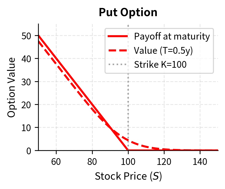
For a European put option with strike and maturity :
where:
- : value of the put option
- : current stock price
- : strike price
- : maturity time
- : current time
- : risk-free interest rate
The terminal condition for the put is the mirror image of the call: the put pays off when the stock price is below the strike. When , the put is certain to pay at maturity, so its current value is the present value of that payment, which equals . When is very large, the stock price is almost certain to remain above the strike, making the put worthless.
The combination of the PDE and these boundary conditions completely determines the option price. Together they form a well-posed mathematical problem: the PDE constrains how the solution must behave in the interior of the domain, while the boundary conditions pin down the solution at the edges. In the next chapter, we'll see how to solve this problem analytically to obtain the famous Black-Scholes formula.
Worked Example: Verifying the PDE
Let's verify that a proposed solution satisfies the Black-Scholes PDE. This exercise builds intuition for what it means to "satisfy" a partial differential equation and demonstrates how to check whether a candidate pricing formula is valid. Consider a simple derivative whose price is , representing a forward contract with zero delivery price and zero interest rates.
We need to check whether satisfies:
where:
- : price of the derivative
- : stock price
- : risk-free interest rate
- : volatility
- : time
Computing the partial derivatives is straightforward since is a simple function:
where:
- : derivative price ()
The time derivative is zero because has no explicit dependence on time. The first derivative with respect to is one because increases linearly with . The second derivative is zero because the relationship is perfectly linear with no curvature.
Substituting into the PDE:
where:
- : model parameters
The left side equals , and the right side is . The equation is satisfied, confirming that the stock price itself is a trivial solution to the BSM PDE. This makes economic sense: holding the stock is a valid "derivative strategy" that trivially satisfies no-arbitrage pricing.
Now consider a more interesting example: a derivative that pays at maturity . Such a derivative might seem exotic, but it illustrates how the PDE handles nonlinear payoffs. We'll verify that a solution of the following form satisfies the PDE:
where:
- : price of the derivative
- : stock price
- : risk-free interest rate
- : volatility
- : maturity time
- : current time
Notice that this formula has an interesting structure: it equals at maturity (when ), satisfying the terminal condition, and it includes an exponential factor that accounts for the time value and volatility effects.
Computing the partial derivatives requires careful application of the chain rule:
where:
- : derivative price ()
- : model parameters
The time derivative is negative because the exponential factor decreases as we approach maturity (when shrinks). The first spatial derivative reflects that the price increases with , at a rate proportional to itself. The second spatial derivative captures the constant curvature of the quadratic relationship.
Substituting these derivatives into the left-hand side (LHS) of the PDE and simplifying:
where:
- LHS: value of left-hand side of PDE
- : derivative price
The algebraic simplification is satisfying: the terms involving cancel (one from the time derivative and one from the gamma term), and the terms involving combine to give exactly what we need.
The right side of the PDE is:
where:
- : risk-free rate
- : derivative price
Both sides are equal, confirming our solution. This example illustrates that derivatives with nonlinear payoffs require appropriate adjustments to their prices, captured by factors that depend on volatility as well as interest rates.
Code Implementation
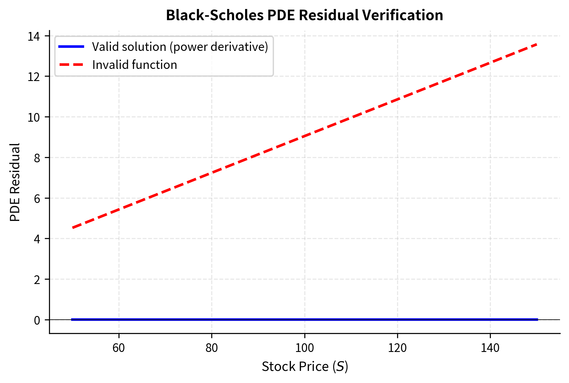
Let's implement a numerical verification that a proposed solution satisfies the Black-Scholes PDE. We'll compute the partial derivatives numerically and check that the PDE residual is close to zero.
Now let's define a test pricing function and verify it satisfies the PDE. We'll use the power payoff derivative from our worked example.
The residual is essentially zero, confirming our analytical solution is correct up to numerical precision.
Let's also test with a function that should not satisfy the PDE, demonstrating that our verification catches invalid solutions.
The non-zero residual confirms that arbitrary functions generally do not satisfy the Black-Scholes PDE.
Visualizing the PDE Residual
Let's create a visualization showing the PDE residual across different stock prices for both valid and invalid pricing functions.
Alternative Derivation: The Replicating Portfolio
There's an alternative way to derive the BSM PDE that provides additional insight and reinforces the economic intuition. Instead of constructing a hedged portfolio of derivative and stock, we can think about replicating the derivative using a portfolio of stock and risk-free bonds. The idea is that if we can perfectly replicate the derivative's payoff using traded securities, then the derivative must have the same price as the replicating portfolio. Otherwise, arbitrage opportunities would exist.
Suppose we want to replicate a derivative using a portfolio of shares of stock and units of risk-free bonds. The portfolio value is:
where:
- : value of the replicating portfolio
- : shares of stock held
- : units of risk-free bonds held
- : stock price
- : value of a risk-free bond
The quantities and can change over time as we continuously adjust the portfolio to maintain replication. This dynamic adjustment is the essence of delta hedging.
For the portfolio to replicate the derivative, we need at all times. The key constraint is that the portfolio must be self-financing: changes in portfolio value come only from price changes, not from adding or removing capital. This means when we rebalance the portfolio, selling some stock to buy bonds or vice versa, the total value must remain unchanged. We can only rearrange what we already own. The self-financing condition is:
where:
- : change in portfolio value
- : shares of stock held
- : change in stock price
- : units of risk-free bonds held
- : change in bond price
This equation says that the change in portfolio value equals the gains from holding stock plus the gains from holding bonds. There is no term for additional capital injection because the portfolio is self-financing.
Recall that represents the risk-free bond dynamics: the bond grows deterministically at the risk-free rate. Substituting the dynamics of and :
where:
- : change in the replicating portfolio value
- : number of shares of stock
- : number of units of risk-free bonds
- : stock drift
- : risk-free interest rate
- : stock volatility
- : Wiener process increment
For replication, we require . The portfolio must change in exactly the same way as the derivative, both in its deterministic component and its random component. Recall the dynamics of the derivative from Itô's lemma:
where:
- : change in derivative price
- : volatility
- : stock price
- : Wiener process increment
Matching the coefficients of the random term gives us the replication condition:
where:
- : shares of stock
- : volatility
- : stock price
- : derivative price
Solving for :
where:
- : number of shares in the replicating portfolio
- : price of the derivative
- : stock price
This confirms that the delta hedge ratio emerges naturally from replication. To replicate the derivative, we must hold exactly delta shares of stock. The remaining portfolio value goes into bonds: . Matching the deterministic components and invoking the self-financing constraint leads to the same PDE. The replicating portfolio approach provides a constructive interpretation: it tells us not only that the derivative price satisfies a PDE, but also how to actually create the derivative synthetically using stock and bonds.
Intuition Behind the PDE Terms
Each term in the Black-Scholes PDE has a financial interpretation that connects the mathematics to economic reasoning. Understanding these interpretations deepens your grasp of why the equation takes the form it does.
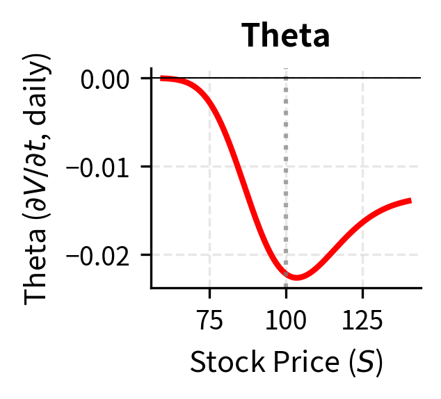
The time derivative represents time decay, often called theta. As time passes, the option's time value erodes, which this term captures. For a call or put option, theta is typically negative: all else equal, the option loses value as expiration approaches because there's less time for favorable stock price movements to occur. The theta term quantifies this inexorable passage of time.
The first-order spatial term appears because the stock price grows on average at the risk-free rate in the risk-neutral world. This term reflects the drift of the stock under the risk-neutral measure. Notice that the drift rate is , not : in the risk-neutral framework, all assets earn the risk-free rate on average. This term captures how the option value changes as the expected stock price evolves.
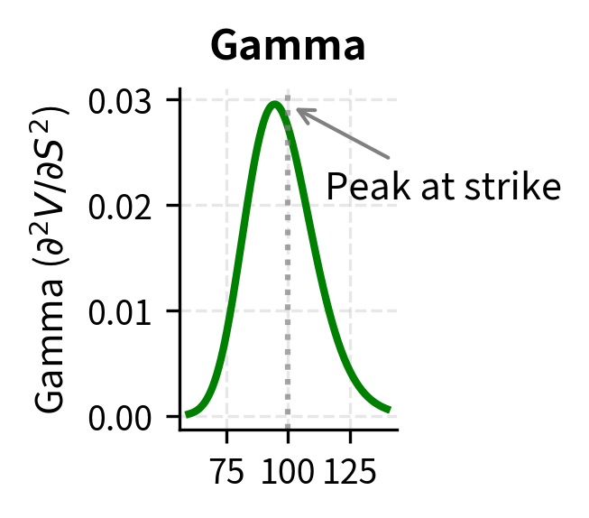
The second-order spatial term captures the convexity effect. Options have curved payoff profiles, and the randomness in stock prices creates value through this curvature. This is related to gamma, which measures how delta changes with the stock price. To understand why convexity creates value, imagine a call option. When the stock price rises, the option becomes more sensitive to further increases (delta rises). When the stock price falls, the option becomes less sensitive to further decreases (delta falls). This asymmetric response means the option benefits more from upward movements than it suffers from downward movements, on average. The gamma term quantifies this benefit from volatility.
The discounting term on the right side reflects that the derivative must be discounted at the risk-free rate. In the risk-neutral world, all assets earn the risk-free rate on average, so the appropriate discount rate is . This term ensures that the present value calculation is consistent with no-arbitrage pricing.
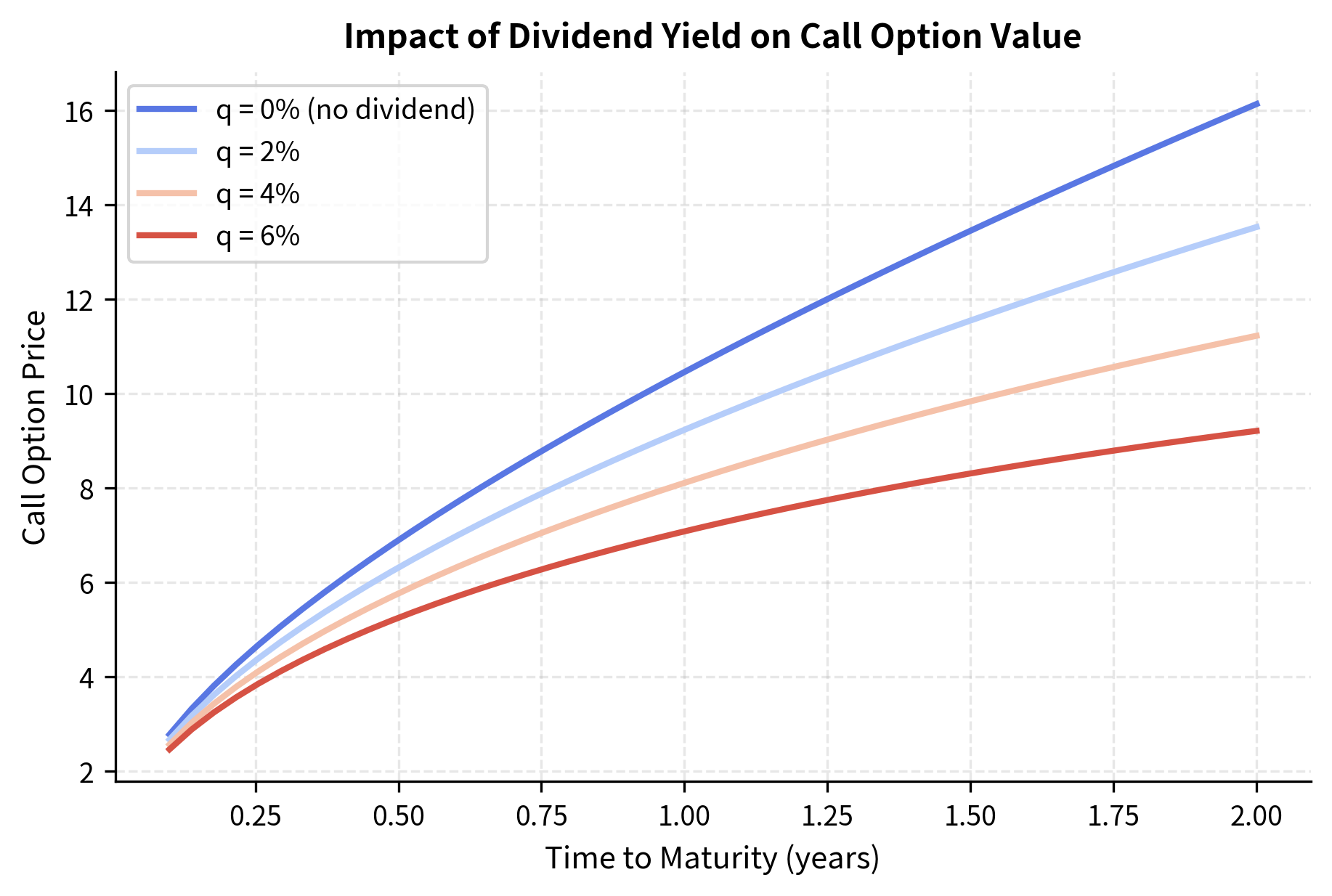
Extending to Dividend-Paying Stocks
The basic BSM PDE assumes the stock pays no dividends. This assumption simplifies the analysis but excludes many important applications, including options on dividend-paying stocks, equity indices, and currencies. For a stock paying continuous dividends at rate , the stock price dynamics become:
where:
- : continuous dividend yield
- : volatility of the underlying stock
- : risk-free interest rate
- : stock price
- : increment of Wiener process under risk-neutral measure
- : small time increment
The key change is that the drift rate under the risk-neutral measure is now rather than . The intuition is that a stock paying dividends at rate provides part of its return through dividend payments rather than price appreciation. In the risk-neutral world, the total expected return (price appreciation plus dividends) must equal , so the expected price appreciation is only .
The modified Black-Scholes PDE is:
where:
- : price of the derivative
- : stock price
- : risk-free interest rate
- : continuous dividend yield
- : volatility of the underlying stock
The intuition is that a stock paying dividends effectively grows slower (by the dividend yield ) than a non-dividend-paying stock, which reduces the drift term in the first-order spatial derivative. This modification is important for pricing options on dividend-paying stocks, equity indices, and currencies (where the foreign interest rate plays the role of a dividend yield, as we discussed in our chapter on foreign exchange markets).
Limitations and Practical Implications
The Black-Scholes-Merton framework transformed derivatives pricing and risk management, but its assumptions impose significant limitations that you must understand. The assumption of constant volatility is perhaps the most problematic: in real markets, volatility changes over time and varies with strike price and maturity. This discrepancy manifests as the volatility smile and volatility surface, which we'll explore in detail in a later chapter. When market-implied volatilities differ systematically from a single constant value, the BSM model cannot perfectly match observed option prices across all strikes.
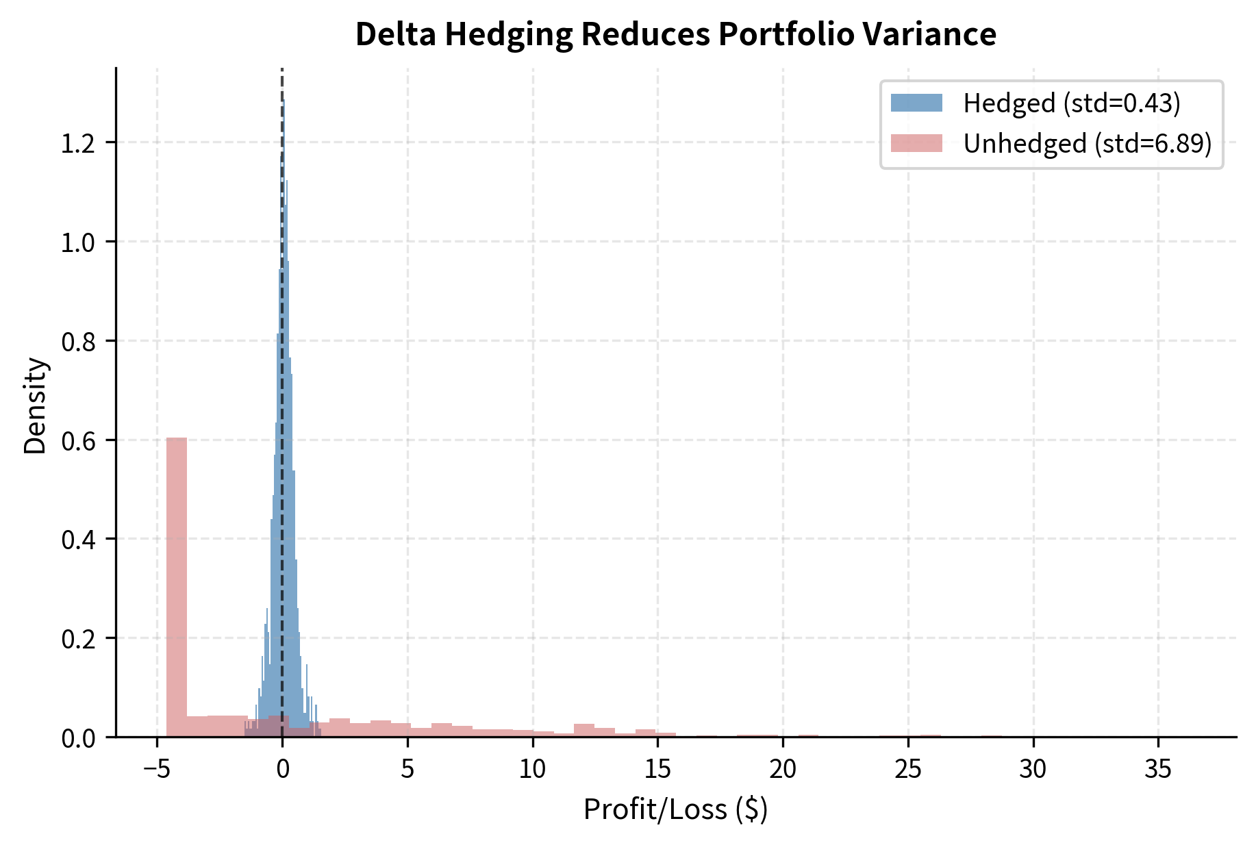
The continuous trading assumption is also unrealistic. Real markets have discrete trading opportunities, transaction costs, and bid-ask spreads. These frictions make perfect delta hedging impossible: you cannot adjust your hedge infinitely often, and each adjustment costs money. The gap between theoretical continuous hedging and practical discrete rebalancing creates residual risk that the basic BSM framework ignores. You can address this through discrete hedging strategies and by accounting for the costs of hedging in your pricing.
Despite these limitations, the BSM PDE remains the foundation of modern derivatives pricing. Its power lies not in its literal accuracy but in providing a systematic framework for thinking about derivative valuation. Extensions and modifications build on this foundation: stochastic volatility models modify the volatility dynamics, jump-diffusion models add discontinuous price movements, and local volatility models allow volatility to depend on price and time. All these approaches either modify the PDE or reframe the problem while retaining the no-arbitrage core insight.
The equation also established delta hedging as the standard approach to managing derivative risk. Even when the assumptions don't hold exactly, the hedge ratios derived from BSM-type models provide useful starting points. The Greeks, which we'll derive from the Black-Scholes formula in an upcoming chapter, give you a systematic way to decompose and manage the various risk exposures embedded in derivative positions.
Summary
This chapter derived the Black-Scholes-Merton partial differential equation, the fundamental equation governing derivative prices under certain idealized conditions. The key insights are:
-
Stock price dynamics: The underlying follows geometric Brownian motion with constant volatility, .
-
Delta hedging eliminates risk: By holding shares of stock against one derivative, we create a portfolio with no exposure to the random term.
-
No-arbitrage implies the PDE: A riskless portfolio must earn the risk-free rate, leading directly to the Black-Scholes PDE.
-
The drift disappears: The expected return does not appear in the final equation; only the volatility and risk-free rate matter for pricing.
-
Boundary conditions specify the derivative: The same PDE applies to all derivatives; what distinguishes calls from puts is the terminal payoff condition.
-
The PDE is linear and backward parabolic: This mathematical structure enables both analytical solutions and efficient numerical methods.
In the next chapter, we'll solve this PDE subject to call and put option boundary conditions, deriving the famous Black-Scholes formula that gives explicit closed-form prices for European options.
Quiz
Ready to test your understanding? Take this quick quiz to reinforce what you've learned about the derivation of the Black-Scholes-Merton PDE.

Comments