

Learn the no-arbitrage principle, replicating portfolios, and risk-neutral probabilities. Master derivative pricing foundations used in quantitative finance.
Choose your expertise level to adjust how many terms are explained. Beginners see more tooltips, experts see fewer to maintain reading flow. Hover over underlined terms for instant definitions.
No-Arbitrage Principle and Risk-Neutral Valuation
The no-arbitrage principle is a foundational concept in quantitative finance. It provides the logical foundation upon which virtually every derivative pricing model rests, from the simple binomial tree to the sophisticated Black-Scholes formula you'll encounter in the next chapters. The principle itself is deceptively simple: there should be no way to make risk-free profits without any initial investment. Yet from this single economic axiom, we can derive precise fair values for complex financial instruments. This approach applies broadly: once we accept that markets should not offer free money, we can deduce the fair prices of options, forwards, swaps, and other derivatives without ever needing to specify how likely different outcomes are.
In this chapter, we develop the no-arbitrage framework systematically. We begin with the economic intuition behind arbitrage and why competitive markets should eliminate it. We then introduce the concept of replicating portfolios, which allows us to price derivatives by constructing equivalent payoffs from simpler instruments. This leads us to the remarkable discovery of risk-neutral probabilities: artificial probabilities under which all assets earn the risk-free rate, enabling us to price any derivative as a simple discounted expected value. The connection between no-arbitrage and risk-neutral valuation is formalized in the Fundamental Theorem of Asset Pricing, a central result in mathematical finance. By the end of this chapter, you will understand not just the mechanics of these pricing techniques, but the deep economic logic that makes them work.
The No-Arbitrage Principle
What Is Arbitrage?
Before we can assert that arbitrage should not exist, we need to define precisely what we mean by the term. Intuitively, an arbitrage is a "sure thing," a trade that guarantees profit without any risk of loss. The formal definition captures this intuition in mathematical language, specifying exactly what conditions must hold for a trading opportunity to qualify as a genuine arbitrage.
An arbitrage opportunity is a trading strategy that requires no initial investment, has no possibility of loss, and has a positive probability of generating a profit.
In more precise mathematical terms, an arbitrage is a portfolio with value at time satisfying:
where:
- : initial portfolio value
- : portfolio value at maturity
- : real-world probability measure
- : time horizon
Let us examine each of these three conditions in turn to understand why they collectively define a "free lunch." The first condition, , states that we start with zero capital. We are not required to put up any money of our own to enter the trade. This might involve borrowing to buy assets, short-selling, or some combination of positions that perfectly offset in terms of initial cost. The second condition, , is the no-loss guarantee. With probability one, meaning in every possible future state of the world, our portfolio will be worth at least zero. We cannot end up owing money. The third condition, , ensures that we actually have something to gain. There must be at least some scenario, with positive probability, in which we end up with a profit. Together, these conditions describe a trading strategy that costs nothing, risks nothing, and sometimes pays off. Such an opportunity would be like finding a money machine: you put nothing in, you risk nothing, and sometimes cash comes out.
A stronger form, called a strong arbitrage or free lunch, satisfies:
where:
- : initial portfolio value
- : portfolio value at maturity
- : real-world probability measure
This stronger form represents an even more flagrant violation of market efficiency. Here you actually receive cash upfront (that is what the negative initial value signifies: the portfolio pays you money when you establish it) and face no future liability. This is even more egregious: someone pays you today, and you owe them nothing tomorrow. In a sense, a strong arbitrage is an immediate free lunch, while the standard arbitrage definition allows for the possibility that the payoff comes later.
Why Arbitrage Should Not Exist
The fundamental economic argument against arbitrage is straightforward: if such opportunities existed, rational investors would immediately exploit them. Markets are populated by profit-seeking traders who constantly scan for mispricings. When an arbitrage appears, it creates a riskless opportunity for profit, and in a world of rational economic agents, such opportunities attract immediate attention. Consider what happens when an arbitrage appears:
- Traders detect the mispricing and execute the arbitrage strategy
- Their buying pressure raises the price of undervalued assets
- Their selling pressure lowers the price of overvalued assets
- Prices adjust until the arbitrage opportunity disappears
This self-correcting mechanism operates continuously in liquid markets. The process is not instantaneous, but in modern financial markets, it operates with remarkable speed. High-frequency trading firms spend billions building systems to detect and exploit arbitrage opportunities in milliseconds. These firms employ sophisticated algorithms, colocated servers, and microwave transmission networks all to gain a few microseconds of advantage in identifying and capturing fleeting mispricings. The fierce competition among these firms ensures that any mispricing is corrected almost instantaneously.
The no-arbitrage principle is therefore not a law of nature but an economic equilibrium condition. Unlike physical laws that hold regardless of human behavior, the absence of arbitrage emerges from the collective actions of market participants. We assume no arbitrage exists because in well-functioning markets, prices should adjust to eliminate it. This assumption becomes our foundational axiom for pricing. When we say that a market is "arbitrage-free," we are making a statement about economic equilibrium rather than physical necessity. Nevertheless, this assumption has proven extraordinarily powerful, allowing us to derive precise pricing relationships that hold remarkably well in practice.
The Law of One Price
A direct consequence of no-arbitrage is the Law of One Price:
Two portfolios that have identical payoffs in all future states of the world must have the same price today.
This principle sounds almost tautological, yet it has far-reaching implications for derivative pricing. The logic behind it is airtight once we accept the no-arbitrage assumption. To see why, suppose portfolio A and portfolio B have the same payoff in every scenario, but . Then you could:
- Buy portfolio A for
- Sell portfolio B for
- Pocket the difference today
- At maturity, your payoffs exactly cancel
The long position in portfolio A delivers exactly what you owe on the short position in portfolio B, regardless of which state of the world materializes. You have perfectly hedged your obligations and locked in a profit equal to the initial price difference. This is an arbitrage: you received cash upfront with no future liability. Therefore, the price difference cannot exist in equilibrium. Any such mispricing would attract arbitrageurs who would trade until prices equalized.
The Law of One Price is the workhorse of derivative pricing. If we can construct a portfolio of simple instruments (stocks, bonds) that replicates the payoff of a derivative, then the derivative must have the same price as that replicating portfolio. This insight transforms the seemingly difficult problem of pricing complex derivatives into the more tractable problem of finding the right combination of simpler assets.
Pricing by Replication
The Replicating Portfolio Approach
The replicating portfolio methodology provides a systematic approach to derivative pricing. Rather than trying to assess the probability of various outcomes or the appropriate discount rate for risky cash flows, we sidestep these thorny issues entirely by constructing a portfolio that mimics the derivative's behavior exactly. The approach proceeds as follows:
- Identify the payoff of the derivative you want to price
- Construct a portfolio of traded assets that produces exactly this payoff
- Calculate the cost of this replicating portfolio
- Conclude that the derivative price equals this cost
This approach is powerful because it converts the problem of pricing an exotic derivative into the simpler problem of finding the right combination of basic instruments. Once we have identified a replicating portfolio, no further analysis is needed. The Law of One Price guarantees that the derivative must trade at the same price as the replication strategy, regardless of investor preferences, probability assessments, or discount rates.
As we discussed in the chapter on Forward and Futures Pricing, we already used this logic implicitly. To price a forward contract on a stock, we showed that buying the stock today and financing it with borrowing replicates the forward's payoff. This replication argument gave us the forward price without any assumptions about the stock's expected return. We never needed to estimate whether the stock was likely to go up or down. The no-arbitrage condition forced the forward price to take a specific value determined solely by the current stock price, the interest rate, and the time to expiration.
A Simple Example: Put-Call Parity
Consider European call and put options with the same strike and expiration on a non-dividend-paying stock. This setting allows us to derive one of the most famous relationships in option pricing, purely through no-arbitrage arguments. At expiration, consider two portfolios:
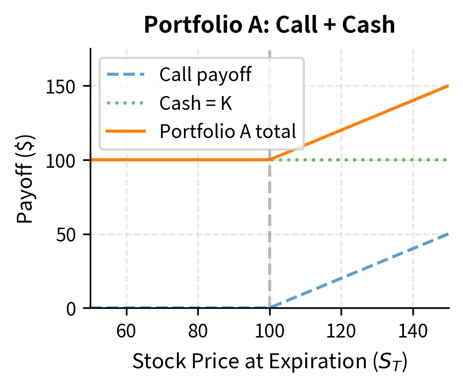
Portfolio A: One call option plus in cash (invested at the risk-free rate)
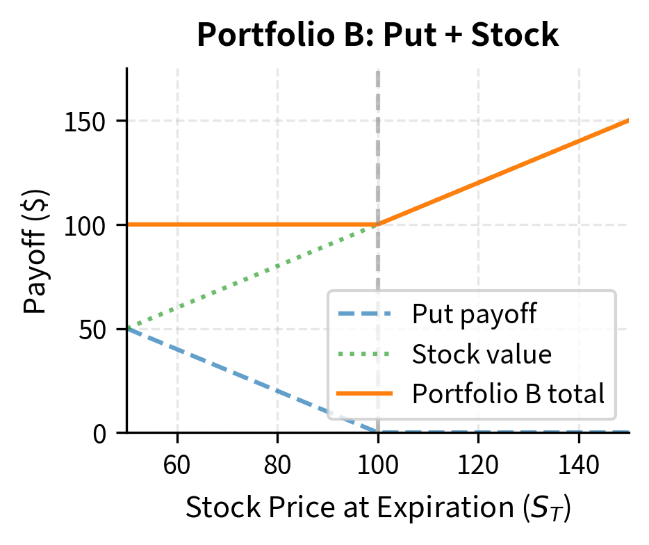
Portfolio B: One put option plus one share of stock
At expiration, let us trace through what each portfolio is worth in both possible scenarios: when the stock finishes above the strike, and when it finishes below. Portfolio A is worth:
where:
- : stock price at expiration
- : strike price
If the stock price exceeds the strike, the call pays and the cash has grown to , giving a total of . If the stock price falls below the strike, the call expires worthless but the cash is worth . Either way, the portfolio is worth the larger of and .
Portfolio B is worth:
where:
- : stock price at expiration
- : strike price
If the stock price falls below the strike, the put pays and the stock is worth , giving a total of . If the stock price exceeds the strike, the put expires worthless but the stock is worth . Once again, the portfolio is worth the larger of and .
Both portfolios have identical payoffs in all states of the world. By the Law of One Price:
where:
- : European call option price
- : European put option price
- : current stock price
- : strike price
- : risk-free interest rate
- : time to expiration
This is put-call parity which you encountered in Part II. Notice we derived it purely from no-arbitrage, without any assumptions about how the stock price moves or what probability distribution governs returns. We did not need to specify a model for stock price dynamics, estimate volatility, or make assumptions about investor risk preferences. The relationship holds simply because both portfolios produce the same future cash flows, and therefore they must cost the same today.
The One-Period Binomial Model
To develop the full machinery of risk-neutral valuation, we need a concrete model of how asset prices evolve. The one-period binomial model is the simplest possible setting, yet it contains all the essential insights that carry over to continuous-time models. By working through this elementary example in detail, we will discover the remarkable phenomenon of risk-neutral pricing, the idea that we can value derivatives using artificial probabilities that make all assets earn the risk-free rate.
Model Setup
Consider a single time period from to . A stock has current price . At time , the stock can take one of two values:
where:
- : stock price at time
- : stock prices in up and down states
- : current stock price
- : up factor ()
- : down factor ()
- : real-world probability of an up move
- : time to expiration
The up factor represents the gross return if the stock increases in value, while the down factor represents the gross return if the stock decreases. Typically we have and , so an "up" move means the stock gains value and a "down" move means it loses value. The actual probability reflects the market's assessment of the stock's prospects. A stock with bright prospects might have a high , while a troubled company might have a low .
There is also a risk-free bond that grows from to . This bond represents a riskless investment that earns the continuously compounded interest rate . Anyone can borrow or lend at this rate.
We want to price a derivative that pays if the stock goes up and if the stock goes down. For a call option with strike :
where:
- : derivative payoff in the up state
- : derivative payoff in the down state
- : stock price in the up state
- : stock price in the down state
- : strike price
The call option pays the difference between the stock price and the strike if this difference is positive, and pays zero otherwise. Our task is to determine what this option should cost today.
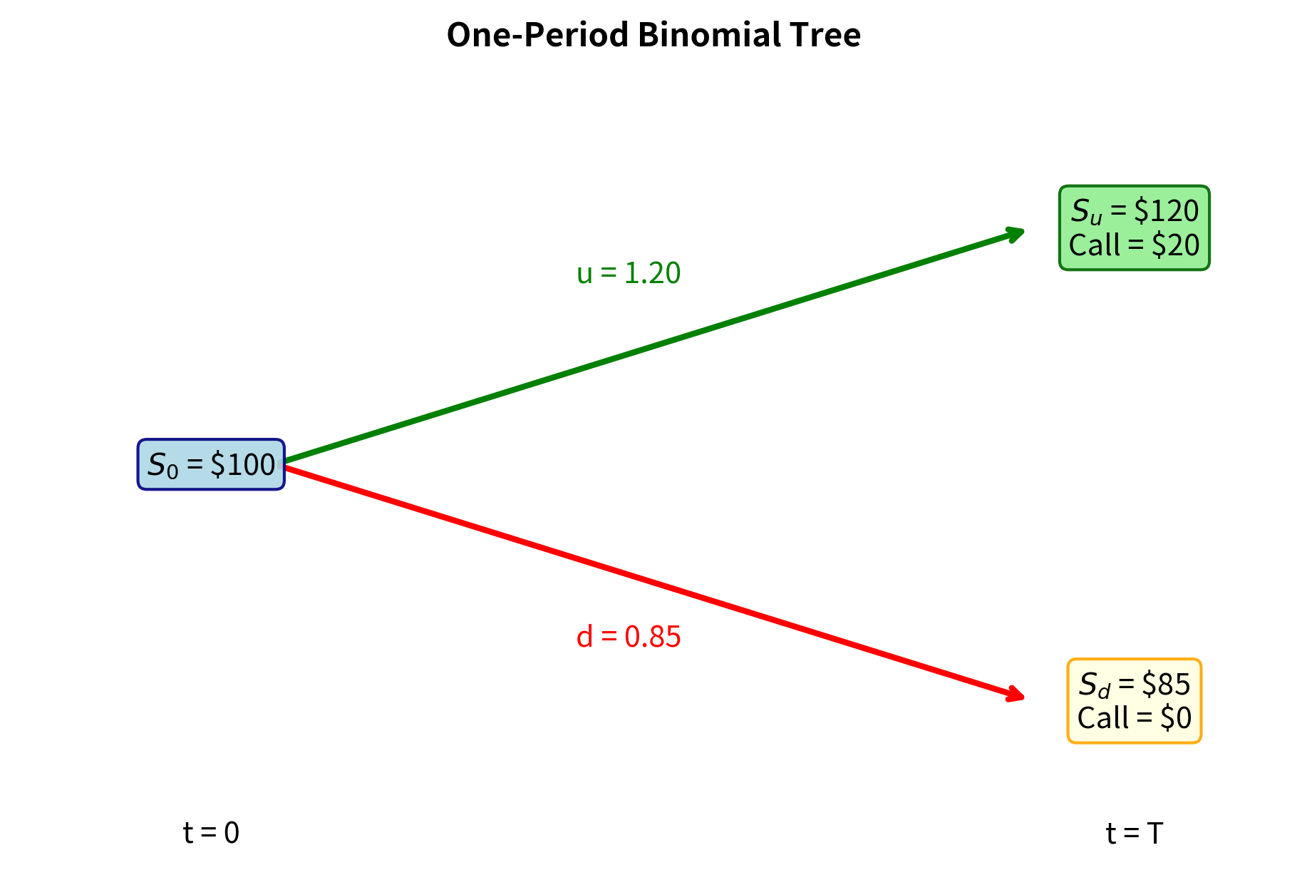
In this example, the stock price can rise to $120 or fall to $85 over the one-year period. The call option yields a $20 payoff in the up state (since $120 > $100) and expires worthless in the down state. The question we face is this: what should someone pay today for the right to receive this contingent payoff one year from now?
Constructing the Replicating Portfolio
We seek a portfolio consisting of shares of stock and dollars invested in the risk-free bond that replicates the option payoff. The Greek letter delta (Δ) represents our position in the stock, while represents our position in the bond. This portfolio must match the option's payoff in both possible states of the world. At time , this portfolio must satisfy:
where:
- : number of shares of stock
- : amount invested in the risk-free bond
- : stock prices in up and down states
- : derivative payoffs in up and down states
- : risk-free rate
- : time to expiration
The first equation says that if the stock goes up, our portfolio (consisting of shares now worth each, plus our bond investment grown to ) must equal the option's payoff . The second equation imposes the same requirement for the down state. We need the portfolio to match the option payoff in both scenarios.
This is a system of two linear equations in two unknowns. Since we have two equations and two unknowns, we can solve for unique values of and . Subtracting the second equation from the first eliminates and allows us to solve for :
where:
- : hedge ratio (shares of stock)
- : amount invested in the risk-free bond
- : option payoffs
- : stock prices at expiration
- : risk-free rate
- : time to expiration
This quantity, called the delta of the option, measures how many shares we need to hold to replicate the option's sensitivity to stock price movements. The formula has an intuitive interpretation: the numerator is how much the option payoff changes between the two states, while the denominator is how much the stock price changes. The ratio tells us how sensitive the option is to stock price movements. For every dollar the stock moves, the option payoff changes by delta dollars.
From either equation, we can solve for :
where:
- : bond investment required for replication
- : derivative payoffs in up and down states
- : stock prices in up and down states
- : hedge ratio
- : risk-free interest rate
- : time to expiration
The two expressions for must give the same answer because we already chose to ensure the equations are consistent. We can use either one for the calculation.
The cost of constructing this portfolio today is:
where:
- : fair value of the derivative today
- : current stock price
- : number of shares
- : bond investment
We buy shares at the current price and invest dollars in the bond. The total outlay is the sum of these two components. By the Law of One Price, this must equal the fair value of the derivative, since the portfolio and the derivative have identical payoffs.
The replicating portfolio holds approximately 0.57 shares of stock and borrows about $46 (the negative bond position indicates borrowing). This leveraged position exactly mimics the option's payoff in both states. If the stock goes up, we hold 0.57 shares worth $120 each which gives us about $68 minus what we owe on our loan, which has grown to about $48 leaving us with $20 exactly the option payoff. If the stock goes down, our 0.57 shares are worth about $48, which exactly offsets our loan obligation, leaving us with nothing, again matching the option payoff. The option must therefore be worth $10.94.
Notice something remarkable: we never used the probability of the up move! The option price depends only on , , , , , and , not on anyone's beliefs about whether the stock will go up or down. This is a key result. Two investors with completely different views about the stock's prospects must still agree on the option's fair price if they both accept the no-arbitrage principle.
The Emergence of Risk-Neutral Probabilities
Let's rearrange our pricing formula algebraically to discover a beautiful alternative representation. We start with the portfolio cost , substitute , and recall that and :
where:
- : derivative price today
- : amount invested in the risk-free bond
- : option payoffs
- : stock prices (current, up, down)
- : up and down factors
- : risk-free rate
- : time to expiration
- : hedge ratio
The algebra may look tedious, but the result is illuminating. We have rewritten the option price as a weighted average of the payoffs, discounted back to the present. If we define a parameter :
where:
- : risk-neutral probability parameter
- : risk-free interest rate
- : time to expiration
- : up and down factors
Then the coefficient for becomes:
where:
- : up and down factors
- : risk-free interest rate
- : time to expiration
- : risk-neutral probability
Thus, the formula simplifies to:
where:
- : the risk-neutral probability of an up move
- : the risk-neutral probability of a down move
- : option payoffs in up and down states
- : risk-free rate
- : time to expiration
This formula has a striking interpretation. The term in brackets, , looks exactly like an expected value: we weight each possible payoff by a probability and sum. The factor discounts this expected value back to the present using the risk-free rate. In other words, the option price equals the discounted expected payoff, where the expectation uses special probabilities and .
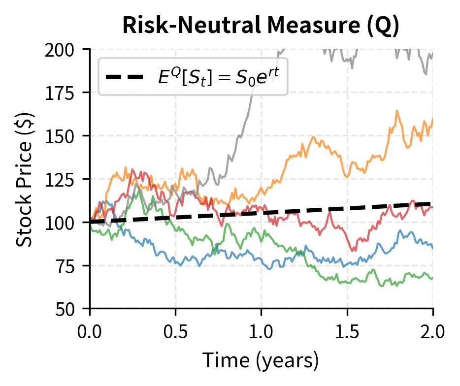
The quantity has a beautiful interpretation. It is the probability that would make the stock's expected return equal to the risk-free rate:
where:
- : expectation under the risk-neutral measure
- : stock price at expiration
- : risk-neutral probability
- : stock prices in up and down states
- : current stock price
- : risk-free rate
This is the defining property of risk-neutral probabilities. Under this special probability measure, which we denote , the stock's expected return equals the risk-free rate. The stock is priced as if investors were indifferent to risk, demanding no premium for bearing uncertainty. Let's verify this:
This is the defining property of risk-neutral probabilities: under these artificial probabilities, all assets earn the risk-free rate in expectation. The derivative price is then simply the discounted expected payoff under this risk-neutral measure. We have discovered a profound result: derivative pricing reduces to calculating an expectation, provided we use the right probability measure.
Key Parameters
The key parameters for the One-Period Binomial Model are:
- S₀: Current stock price. The base value from which up and down movements occur.
- u, d: Up and down factors. Ratios determining the stock price in the next period (, ).
- r: Risk-free interest rate. The rate at which the bond grows and future cash flows are discounted.
- T: Time to expiration in years.
- K: Strike price of the option.
- q: Risk-neutral probability. The theoretical probability of an up move that equates the expected stock return to the risk-free rate.
Understanding Risk-Neutral Probabilities
What Risk-Neutral Probabilities Are Not
Risk-neutral probabilities are emphatically not real-world probabilities. This point deserves emphasis because it is a common source of confusion. They do not represent:
- The actual likelihood of the stock going up or down
- Any investor's subjective beliefs about future prices
- Historical frequencies of up and down moves
In our example, says nothing about whether the stock will actually rise or fall. If a stock analyst believes there's an 80% chance the stock goes up, that real-world probability is irrelevant for pricing. The option price is 10.94. This is counterintuitive at first. How can the option price not depend on the probability the stock goes up? After all, a call option is worth more if the stock is more likely to rise. If you believe the stock has an 80% chance of reaching $120, shouldn't you pay more for the call than someone who thinks there's only a 40% chance?
The Resolution: Risk Adjustments
The resolution lies in recognizing that the replication argument works regardless of probabilities because we're constructing a hedge that eliminates risk. When we hold shares against the option, the portfolio is perfectly hedged: it produces the same value whether the stock goes up or down. The hedged position is completely insensitive to the stock's direction.
In equilibrium, the cost of this hedged portfolio must be the price of the derivative. The hedge completely eliminates exposure to the up/down uncertainty, so the underlying probabilities become irrelevant to the pricing. Since we can perfectly replicate the option using the stock and bond, the option's price is pinned down by the replication cost, not by probability assessments.
Another way to see this: risk-neutral probabilities implicitly adjust for risk preferences. In the real world, investors are typically risk-averse. They demand higher expected returns from risky assets to compensate for bearing risk. Stocks have expected returns above the risk-free rate precisely because investors require this risk premium. A stock that is expected to return 10% per year includes both the time value of money (perhaps 5%) and a risk premium (another 5%) that compensates for the possibility of loss.
Risk-neutral probabilities mathematically combine two effects:
- Real-world probabilities of outcomes
- Risk adjustments that discount risky payoffs more heavily
The net result is a probability measure under which all assets earn the risk-free rate. The risk premium has been baked into the probabilities rather than the discount rate. Instead of using high real-world probabilities and a high discount rate (reflecting risk aversion), we use lower risk-neutral probabilities and a low discount rate (the risk-free rate). Both approaches give the same answer because they capture the same economic reality from different angles.
Two Equivalent Approaches to Pricing
We now have two mathematically equivalent ways to price derivatives:
Real-World Approach: Compute expected payoffs under actual probabilities and discount at a risk-adjusted rate
where:
- : derivative price today
- : risk-adjusted discount rate
- : time to expiration
- : expectation under real-world probability measure
- : derivative payoff at time
This approach requires knowing the real-world probabilities and determining the appropriate risk-adjusted discount rate for the specific payoff pattern. The discount rate must reflect not just the time value of money but also the riskiness of the cash flows and how that risk relates to the broader market.
Risk-Neutral Approach: Compute expected payoffs under risk-neutral probabilities and discount at the risk-free rate
where:
- : derivative price today
- : risk-free interest rate
- : time to expiration
- : expectation under risk-neutral probability measure
- : derivative payoff at time
This approach uses the artificial risk-neutral probabilities and always discounts at the risk-free rate , regardless of the derivative's risk characteristics.
The risk-neutral approach is vastly more practical because:
- We don't need to estimate real-world probabilities (notoriously difficult)
- We don't need to determine the appropriate risk premium for each derivative
- The risk-free rate is directly observable
The entire complexity of risk preferences and probability estimation gets absorbed into finding the right risk-neutral measure, which is determined by no-arbitrage conditions. Rather than solving the hard problem of estimating probabilities and discount rates, we solve the tractable problem of finding the replicating portfolio or equivalently the risk-neutral measure.
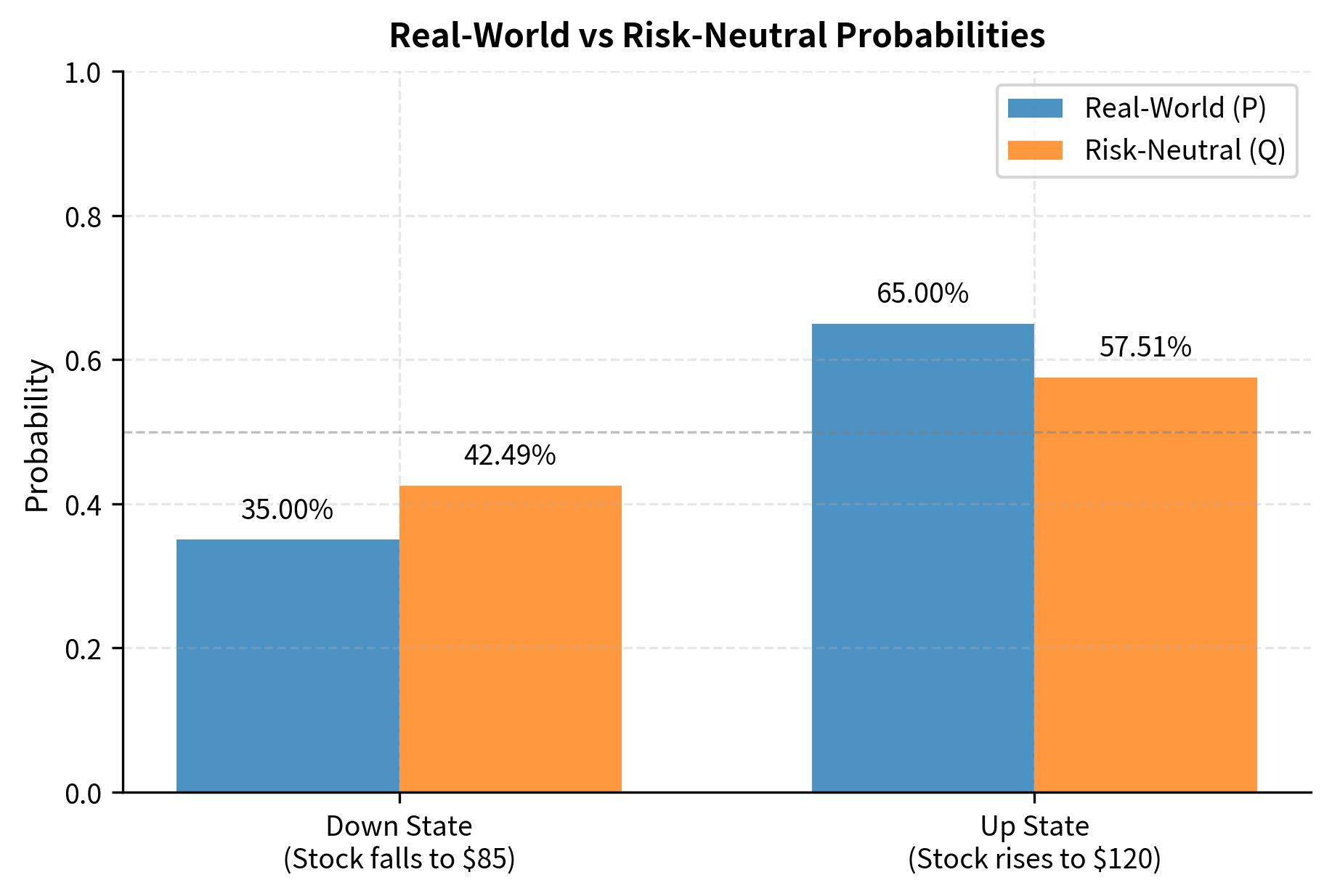
The figure illustrates a key insight: risk-neutral probabilities typically assign more weight to adverse outcomes than real-world probabilities. In this example, even if we believe there's a 65% chance of the stock rising, the risk-neutral probability of an up move is only 57%. This shift reflects the risk premium embedded in stock prices. Because investors are risk-averse, they bid down stock prices below their expected discounted values, which manifests as a shift in the risk-neutral probabilities toward unfavorable outcomes.
The Fundamental Theorem of Asset Pricing
The connection between no-arbitrage and risk-neutral pricing is not a coincidence. It is formalized in one of the most important theoretical results in mathematical finance. This theorem establishes that our two key concepts, absence of arbitrage and existence of risk-neutral probabilities, are logically equivalent.
Statement of the Theorem
A market model is arbitrage-free if and only if there exists at least one probability measure , equivalent to the real-world measure , under which all discounted asset prices are martingales.
This theorem is profound because it connects an economic concept (no free lunch) with a mathematical structure (martingale measure). Let's unpack this statement:
Arbitrage-free: No trading strategy can generate risk-free profits from zero initial capital. This is the economic condition we have been assuming throughout.
Equivalent probability measure: A measure that assigns positive probability to exactly the same events as . If something is possible under , it's possible under , and vice versa. This requirement ensures that the risk-neutral world doesn't consider impossible events to be possible, or vice versa.
Martingale: A stochastic process where the expected future value, given current information, equals the current value. Intuitively, a martingale is a "fair game" with no systematic drift. For discounted asset prices:
where:
- : expectation under the risk-neutral measure
- : stock prices at time and
- : risk-free bond prices at time and
- : information available at time
This equation says the discounted stock price is a "fair game" under : you don't expect it to systematically drift up or down in discounted terms. When we divide by the bond price, we are measuring the stock's value in units of the risk-free asset. Under the risk-neutral measure, this relative value is expected to stay constant.
Implications for Pricing
The Fundamental Theorem has profound implications for both theory and practice:
-
Existence of risk-neutral measure: If markets are arbitrage-free (as we assume), then risk-neutral probabilities exist. We can always find a measure for pricing. This is comforting: our pricing approach is not an arbitrary trick but rests on solid theoretical foundations.
-
Uniqueness and completeness: If the risk-neutral measure is unique, the market is complete, meaning every derivative can be perfectly replicated. If multiple risk-neutral measures exist, the market is incomplete, and there's a range of arbitrage-free prices. In incomplete markets, different risk-neutral measures correspond to different ways of pricing risk, and the no-arbitrage condition alone doesn't pin down a unique price.
-
Pricing formula: Under , any derivative paying at time has price:
where:
- : derivative price today
- : derivative payoff at maturity
- : risk-free rate
- : time to maturity
- : expectation under the risk-neutral measure
This elegant formula reduces derivative pricing to computing a single expectation, provided we can characterize the risk-neutral dynamics of the underlying. All the complexity of hedging and replication gets absorbed into the change of probability measure.
In our binomial model, the market is complete: there are two states and two assets (stock and bond), so we can perfectly replicate any payoff. The risk-neutral measure is unique, given by the probability we derived. With two assets and two states, we have exactly enough instruments to span all possible payoffs.
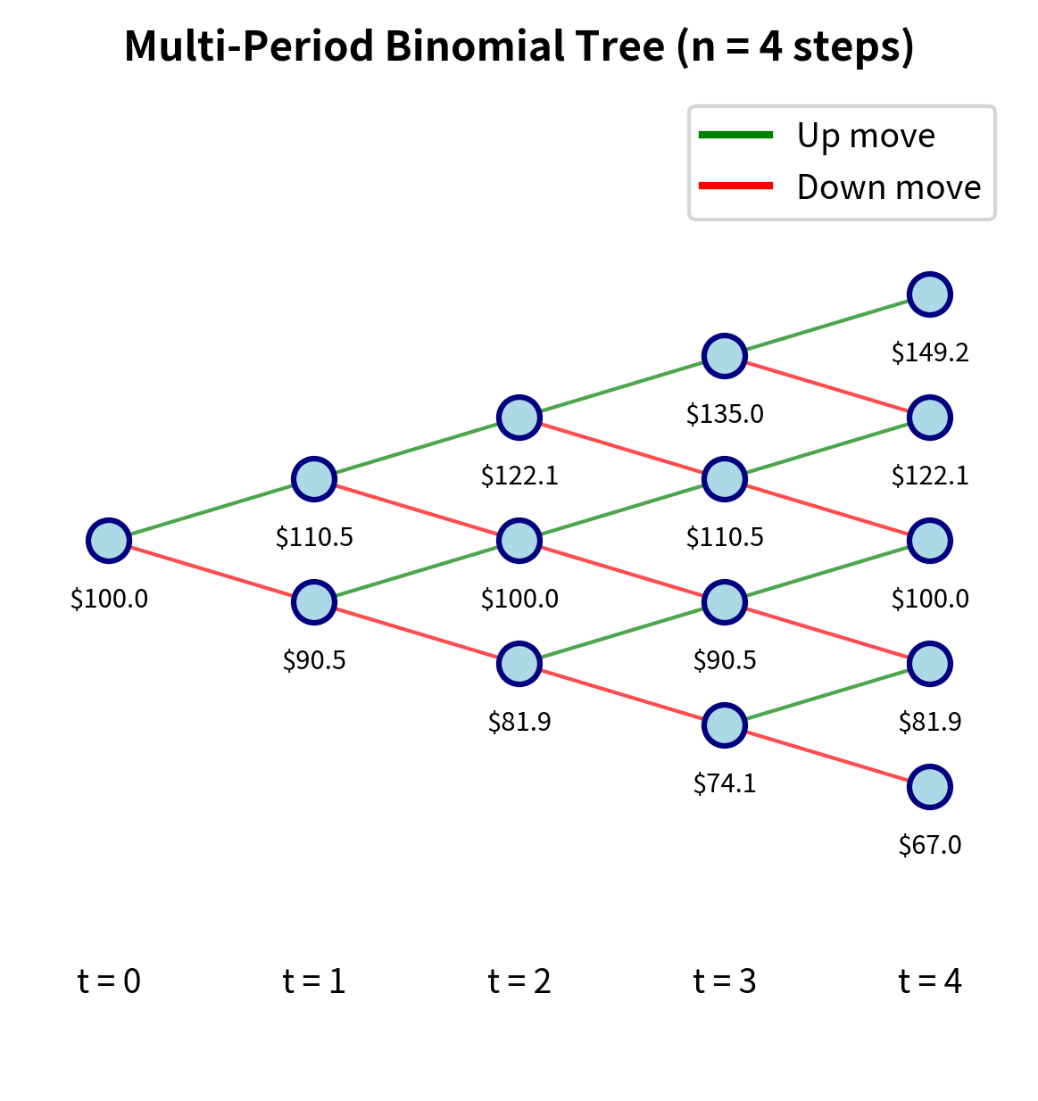
Multi-Period Binomial Model
The one-period model extends naturally to multiple periods, providing a flexible framework for pricing American options and path-dependent derivatives. By chaining together many small one-period models, we can approximate arbitrarily complex price dynamics while maintaining the tractability of the binomial approach.
Model Structure
Divide the time to expiration into steps, each of length . At each step, the stock either goes up by factor or down by factor . After steps, the stock can be at any of different price levels. The tree structure grows exponentially: at step , there are possible stock prices, corresponding to having experienced up moves and down moves for each from 0 to .
The algorithm works by backward induction, starting from the known payoffs at expiration and working back to the present. This is the natural approach because at expiration we know exactly what the option is worth (its intrinsic value), and at each earlier node we can compute the value from the risk-neutral formula. The steps are:
- Calculate all possible stock prices at expiration
- Compute the option payoff at each terminal node
- Work backwards: at each earlier node, the option value is the discounted risk-neutral expectation of its values at the two successor nodes
The 50-step binomial tree yields call and put prices that satisfy put-call parity. The calculated prices reflect the discrete approximations of the continuous process, and as we increase the number of steps, these values will converge to the Black-Scholes prices. The fact that put-call parity holds confirms that our implementation is internally consistent.
Convergence to Continuous Time
An important property of the binomial model is that as we increase the number of steps, the discrete model converges to a continuous-time model. This convergence is not merely approximate: with the right choice of parameters, the binomial model converges exactly to the continuous-time geometric Brownian motion model. If we choose:
where:
- : up and down factors
- : volatility of the stock
- : length of each time step
Then as and , the binomial stock price process converges to geometric Brownian motion:
where:
- : change in stock price
- : stock price at time
- : drift (expected return)
- : small time increment
- : volatility
- : increment of a standard Brownian motion
This is the process we studied in the previous chapter on Brownian Motion and Random Walk Models. The binomial model can be viewed as a discretization of this continuous process. As we make the time steps smaller and smaller, the discrete jumps of the binomial model approximate the continuous fluctuations of Brownian motion with increasing accuracy. The binomial option prices converge to the Black-Scholes prices, which we'll derive in the next chapter.
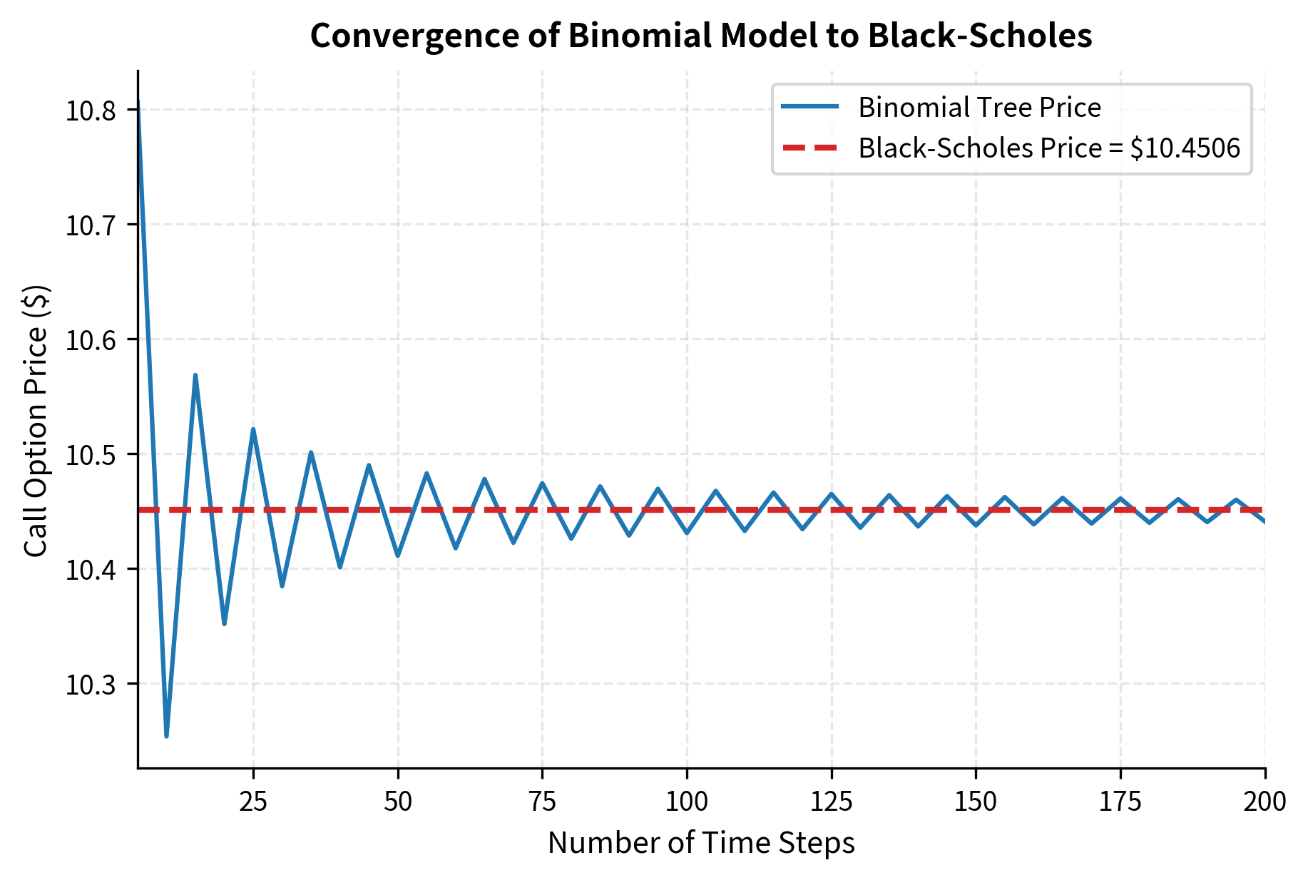
The oscillation in binomial prices, visible for small numbers of steps, occurs because the discrete lattice can position the strike price differently relative to the nodes. Depending on whether the strike falls near a node or between nodes, the approximation error can be larger or smaller. These oscillations dampen as the number of steps increases, and the price converges smoothly to the Black-Scholes value. In practice, 50-100 steps typically provide sufficient accuracy for most applications.
Key Parameters
The key parameters for the Multi-Period Binomial Model are:
- n: Number of time steps. Controls the resolution of the tree; higher converges to continuous-time prices.
- σ: Volatility of the underlying asset. Used to calculate the up and down factors ( and ) so that the tree matches the asset's variance.
- Δt: Time step size (). The duration of each step in the tree; as the model converges to the continuous-time geometric Brownian motion.
Risk-Neutral Valuation in Continuous Time
The discrete binomial framework extends naturally to continuous time, where calculus replaces algebra and Brownian motion replaces discrete jumps. The core insight remains the same: we can change probability measures to simplify derivative pricing.
The Girsanov Theorem Connection
In continuous time, the transition from real-world to risk-neutral probabilities involves changing the drift of the Brownian motion. This change of measure, which generalizes what we did in the discrete binomial model, is accomplished through the Girsanov theorem. Under the real-world measure , the stock follows:
where:
- : change in stock price
- : stock price at time
- : expected return under measure
- : small time increment
- : volatility
- : Brownian increment under measure
Here the drift reflects the stock's actual expected return, which typically exceeds the risk-free rate due to the equity risk premium.
The Girsanov theorem, a fundamental result in stochastic calculus, tells us we can change to an equivalent measure under which:
where:
- : change in stock price
- : risk-free interest rate
- : stock price at time
- : small time increment
- : volatility
- : Brownian increment under risk-neutral measure
The drift changes from to , but the volatility remains unchanged. This is crucial: the change of measure affects the expected return but not the magnitude of the random fluctuations. Under this risk-neutral measure, the stock earns the risk-free rate, and we can price any derivative as:
where:
- : price of the derivative
- : risk-free interest rate
- : time to expiration
- : expectation under risk-neutral measure
- : payoff at expiration
The relationship between the two Brownian motions involves the market price of risk :
where:
- : Brownian increments under measures and
- : market price of risk
- : small time increment
This quantity measures the excess return per unit of volatility that investors demand for bearing stock price risk. A high market price of risk indicates that investors require substantial compensation for bearing uncertainty. The Girsanov change of measure essentially absorbs this risk premium into the probability measure itself, transforming a world where risky assets earn excess returns into a world where everything earns the risk-free rate.

We'll explore these ideas further when we derive the Black-Scholes-Merton PDE in the next chapter, where the continuous-time hedging argument leads to the same conclusion through a different route.
Practical Applications
The theoretical framework developed in this chapter has immediate practical value. Risk-neutral valuation provides the conceptual foundation for pricing derivatives across asset classes and complexity levels.
Pricing Complex Derivatives
Risk-neutral valuation provides a unified framework for pricing virtually any derivative. The conceptual approach is the same whether we are pricing a simple European call or a complex path-dependent exotic option:
- Specify the risk-neutral dynamics of underlying assets
- Determine the derivative's payoff as a function of the underlying's path
- Compute the discounted expected payoff under the risk-neutral measure
For European options with nice analytical forms, we can often derive closed-form pricing formulas. The Black-Scholes formula for European calls and puts is the most famous example, but similar formulas exist for many other products. For more complex derivatives, we use numerical methods:
- Binomial/trinomial trees for American options and simple path-dependencies
- Monte Carlo simulation for path-dependent options with many underlying assets
- Finite difference methods for solving the pricing PDE directly
These numerical techniques, which we'll cover in detail in upcoming chapters, all rest on the risk-neutral valuation foundation established here. The theoretical framework is the same; only the computational implementation differs.
Calibration to Market Prices
In practice, we don't simply pick model parameters and compute prices. Instead, we:
- Observe market prices of liquid options
- Find risk-neutral parameters that match these prices
- Use the calibrated model to price exotic derivatives
For example, if we observe call option prices for various strikes, we can back out the implied volatility that makes the Black-Scholes formula match each price. The resulting implied volatility surface tells us about the market's risk-neutral expectations for future stock price movements. Different strikes and expirations typically imply different volatilities, revealing the market's view of the full probability distribution, not just its variance.
This calibration approach is essential because it ensures our model prices are consistent with liquid market prices, reducing arbitrage opportunities between our model and the market. A model that produces prices inconsistent with observed market prices is effectively creating phantom arbitrage opportunities that don't actually exist.
Limitations and Practical Considerations
The no-arbitrage framework provides powerful pricing tools, but you must understand its limitations. Real markets differ from the idealized conditions assumed in our derivations.
Model Dependence
While no-arbitrage restricts prices significantly, it does not uniquely determine them for most derivatives. The risk-neutral approach requires specifying how underlying assets evolve under the risk-neutral measure. Different model choices, such as geometric Brownian motion versus jump-diffusion versus stochastic volatility, lead to different prices for the same derivative.
For simple European options on liquid underlyings, this model dependence is manageable because we calibrate to market prices. If we use the implied volatility from the market, we will match the market price by construction. For exotic derivatives or illiquid underlyings, model risk becomes a significant concern. Two equally plausible models might produce substantially different prices, and there's no way to know which is "correct" until the derivative expires.
We address model risk through several strategies: using multiple models and examining the range of prices, stress testing against alternative specifications, and adding model uncertainty premiums to quoted prices. The more exotic the derivative, the wider the uncertainty band around its "fair" price.
Market Frictions
The no-arbitrage framework assumes idealized conditions:
- No transaction costs
- Unlimited borrowing and lending at the risk-free rate
- Perfect divisibility of assets
- No restrictions on short selling
- Continuous trading
Real markets violate all these assumptions. Transaction costs create bid-ask spreads that allow a range of prices to coexist without arbitrage. Funding costs differ from the risk-free rate and vary across counterparties. Short-selling restrictions can prevent the execution of arbitrage strategies. Assets cannot be traded in infinitesimal quantities.
These frictions don't invalidate the framework, but they do create no-arbitrage bounds, rather than unique prices. A derivative might have any price within these bounds without triggering arbitrage. The bounds are typically tight for liquid instruments but can be wide for exotic or illiquid products.
Credit Risk
The analysis implicitly assumes all parties fulfill their obligations. In practice, counterparty credit risk affects derivative pricing. An option purchased from a risky counterparty is worth less than one from a risk-free entity because there's a chance the counterparty defaults before paying the option's value.
Modern derivative valuation incorporates credit valuation adjustments (CVA) and other XVA adjustments that modify the idealized risk-neutral price to account for credit, funding, and capital costs. These adjustments have become increasingly important since the 2008 financial crisis highlighted the significance of counterparty risk.
Summary
This chapter established the theoretical foundations that underpin all derivative pricing:
The no-arbitrage principle asserts that markets should not permit risk-free profits from zero capital. This simple economic axiom, enforced by competitive trading, places powerful restrictions on relative prices of financial instruments.
The Law of One Price follows directly: portfolios with identical payoffs must have identical prices. This enables pricing by replication: find a portfolio of simple instruments that mimics the derivative, and its cost is the derivative's fair value.
The binomial model demonstrates these principles concretely. By constructing a hedging portfolio that replicates option payoffs, we derive prices without knowing or using real-world probabilities.
Risk-neutral probabilities emerge from the replication argument. These artificial probabilities make all assets earn the risk-free rate in expectation, allowing us to price derivatives as simply discounted expected payoffs. They incorporate risk adjustments implicitly, absorbing investor risk preferences into the probability measure.
The Fundamental Theorem of Asset Pricing formalizes the no-arbitrage/risk-neutral connection: absence of arbitrage is equivalent to existence of a risk-neutral measure under which discounted prices are martingales.
These ideas extend naturally to continuous time, where the change of measure from real-world to risk-neutral probabilities is governed by Girsanov's theorem. In the next chapter, we'll use these principles to derive the celebrated Black-Scholes-Merton partial differential equation, which opened the door to modern quantitative finance.
Quiz
Ready to test your understanding? Take this quick quiz to reinforce what you've learned about no-arbitrage pricing and risk-neutral valuation.

Comments