

Master Itô's Lemma with complete derivations and Python simulations. Learn stochastic calculus, geometric Brownian motion, and derivative pricing foundations.
Choose your expertise level to adjust how many terms are explained. Beginners see more tooltips, experts see fewer to maintain reading flow. Hover over underlined terms for instant definitions.
Itô's Lemma and Stochastic Calculus.
In the previous chapter, we explored Brownian motion, the mathematical foundation for modeling random price movements. We saw that Brownian motion has continuous but nowhere-differentiable paths, creating a fundamental problem: how do we apply calculus to functions of processes that cannot be differentiated in the classical sense?
Stochastic calculus, developed by Kiyoshi Itô in the 1940s, extends ordinary calculus to random processes. Itô's Lemma serves as the chain rule for this framework. Just as the ordinary chain rule tells us how to differentiate composite functions, Itô's Lemma tells us how functions of stochastic processes evolve over time.
Quantitative finance uses Itô's Lemma to derive derivative price dynamics. For an asset following geometric Brownian motion, Itô's Lemma shows how options and other derivatives behave. It will be the key tool we use in the next chapter to derive the Black-Scholes-Merton partial differential equation.
Stochastic Differential Equations
Building on our understanding of Brownian motion from the previous chapter, we now formalize how to describe the continuous-time evolution of random processes. We need to express how a quantity changes when it involves both predictable trends and random fluctuations. A stochastic differential equation (SDE) provides exactly this capability by expressing the instantaneous change in a process as the sum of a deterministic component and a random component. This dual structure captures the essential nature of financial markets, where prices exhibit both systematic tendencies and random fluctuations.
An Itô process is a stochastic process that can be written in the form:
where:
-
: the stochastic process value at time
-
: the drift coefficient (expected instantaneous change)
-
: the diffusion coefficient (instantaneous volatility)
-
: standard Brownian motion
-
: infinitesimal time increment
-
: infinitesimal Brownian increment
The differential notation represents the infinitesimal change in over an infinitesimally small time interval . This notation provides intuition and leads to correct results when following the rules of stochastic calculus, despite lacking traditional rigor. The notation can be made rigorous through the theory of stochastic integration, but for practical purposes, working with differentials and following consistent rules yields reliable answers.
The two terms in an SDE have distinct interpretations:
-
Drift term (): The expected change in the process over time. This is the deterministic trend component that would remain if we removed all randomness. You can think of it as the underlying direction in which the process is being pushed. If we observed many sample paths and averaged them, the drift would be what remains.
-
Diffusion term (): The random fluctuation around the drift. Since has variance , the diffusion coefficient controls the magnitude of random shocks. Larger values of mean the process experiences more substantial random perturbations at each instant.
Arithmetic Brownian Motion
The simplest SDE has constant coefficients:
where:
-
: value of the process at time
-
: constant drift rate
-
: constant volatility
-
: infinitesimal time step
-
: infinitesimal Brownian increment
This is arithmetic Brownian motion, also called Brownian motion with drift. The process drifts upward at rate while fluctuating randomly with volatility . Because both the drift and diffusion coefficients are constants that do not depend on the current level of , the process can wander anywhere on the real line. As we discussed in the previous chapter, this process can take negative values, making it unsuitable for modeling asset prices directly. After all, stock prices cannot become negative, yet arithmetic Brownian motion places no lower bound on the values it can reach.
Geometric Brownian Motion
A more realistic model for asset prices is geometric Brownian motion (GBM), which we introduced conceptually in the previous chapter. The key innovation in GBM is that both the drift and diffusion scale with the current price level:
where:
-
: asset price at time
-
: constant percentage drift
-
: constant percentage volatility
-
: infinitesimal time increment
-
: Brownian motion increment
Here, both the drift and diffusion are proportional to the current price level. This proportionality fundamentally changes the behavior of the process and ensures several desirable properties:
-
The process remains strictly positive (prices cannot go negative) because the multiplicative structure prevents the process from crossing zero
-
Percentage returns, not absolute returns, have constant volatility, which matches empirical observations about financial markets
-
The model exhibits the multiplicative dynamics observed in real markets, where a 10% gain followed by a 10% loss does not return you to your starting point
We can factor out to see that the percentage change follows a simple form:
where:
-
: instantaneous percentage return
-
: drift rate
-
: infinitesimal time increment
-
: volatility parameter
-
: Brownian motion increment
This equation says the instantaneous percentage return has drift and volatility . This means volatility is usually a percentage of price, not an absolute dollar amount. A 20% volatility means that daily percentage moves have a standard deviation related to this 20% annual figure, regardless of whether the stock trades at 1,000 This matches the stylized facts of financial returns we covered in Chapter 1 of this part.
Why Ordinary Calculus Fails
Before deriving Itô's Lemma, we need to understand why ordinary calculus cannot be applied directly to stochastic processes. Standard calculus fails because Brownian motion paths are irregular. Unlike smooth functions that we encounter in standard calculus, Brownian motion exhibits roughness at every scale. This roughness changes how we think about differentiation and integration.
The Taylor Expansion Approach
Suppose we have a smooth function and we want to know how changes when changes by a small amount . The strategy in ordinary calculus is to approximate the function locally using its derivatives. The Taylor expansion gives us this approximation:
where:
-
: value of the function at
-
: first derivative of
-
: second derivative of
-
: small change in
In ordinary calculus, when we take the limit , all terms beyond the first-order term become negligible. This is because higher powers of small quantities become vanishingly small compared to the first power. The resulting differential form is:
where:
- : differential change in the function
- : first derivative of with respect to
- : differential change in
This works because is infinitesimally smaller than . We have . The second-order term vanishes in the limit, leaving only the familiar first-order derivative expression that forms the foundation of differential calculus.
The Problem with Brownian Motion
Now consider what happens when is replaced by a Brownian motion . Over a small time interval , the change in Brownian motion is . While the expected value of is zero, its variance is . This variance property is the source of all the complications that follow.
Here's the critical observation: what is the expected value of ? To answer this, we use the fundamental relationship between moments:
where:
-
: expected value operator
-
: increment of Brownian motion over time
-
: variance operator
This result has important consequences: behaves like , not like . When we sum many such terms over an interval, the second-order terms don't vanish as they would in ordinary calculus. Instead, they accumulate to a finite, deterministic quantity. This accumulation is the fundamental reason why the ordinary chain rule fails for stochastic processes and why we need a modified version, namely Itô's Lemma.
The Quadratic Variation of Brownian Motion
Let's make the preceding observation mathematically precise. We want to understand what happens when we sum up squared increments of Brownian motion over an interval. Partition the interval into subintervals of length . The quadratic variation of Brownian motion over is defined as the sum of squared increments:
where:
-
: number of subintervals in the partition
-
: value of Brownian motion at time
-
: increment of Brownian motion over the -th interval
Each squared increment has expected value . The variance of each squared increment is . This variance result follows from the fact that if is a standard normal random variable, then follows a chi-squared distribution with 1 degree of freedom, which has variance 2.
The sum has expected value and variance given by:
where:
-
: number of subintervals
-
: length of each subinterval ()
-
: total time horizon
The variance of the sum involves a key computation:
where:
-
: variance operator
-
: variance of a squared Brownian increment
As the partition becomes finer (as increases), something important occurs. The variance goes to zero while the expected value stays fixed at . This means the sum converges not just in expectation but in a stronger sense. The sum converges in mean square to the constant :
where:
-
: convergence in mean square ( norm)
-
: deterministic limit of the quadratic variation
The symbolic result distinguishes stochastic from ordinary calculus. In ordinary calculus, the quadratic variation of any smooth function is zero. In stochastic calculus, Brownian motion has positive, finite quadratic variation equal to the length of the time interval. This non-zero quadratic variation is what forces us to include second-order terms in our calculus.
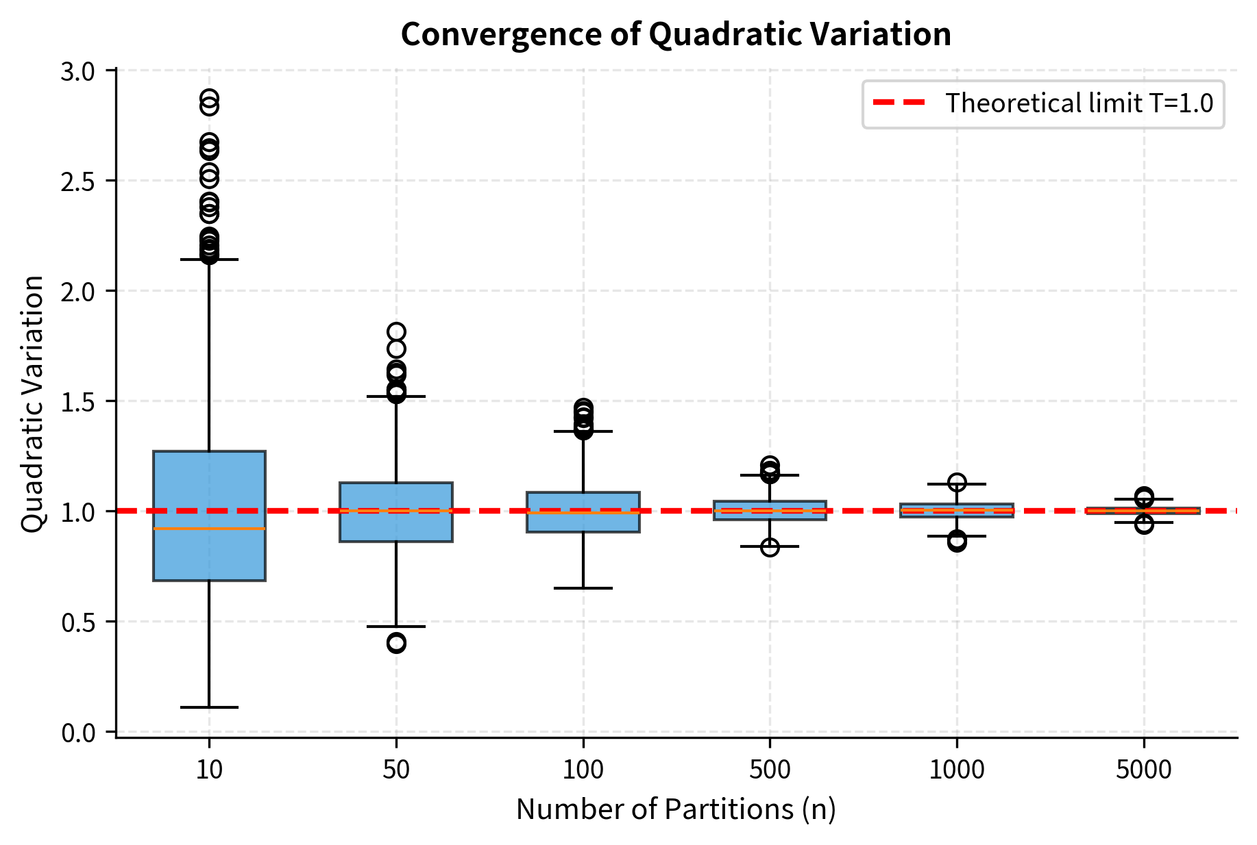
The simulation confirms that the quadratic variation converges to with decreasing variance as the partition becomes finer. The standard deviation follows the theoretical prediction of . This numerical evidence reinforces the theoretical result: as we refine our partition, the sum of squared Brownian increments becomes increasingly concentrated around the deterministic value .
Derivation of Itô's Lemma
Now we derive Itô's Lemma, which tells us how to compute the differential of a function when follows an Itô process. This derivation follows the logic of Taylor expansion but carefully accounts for the non-vanishing quadratic variation of Brownian motion that we just established.
Setup
Let satisfy the SDE:
where:
-
: stochastic process value
-
: drift coefficient
-
: diffusion coefficient
-
: infinitesimal time increment
-
: Brownian increment
and let be a function that is twice continuously differentiable in and once continuously differentiable in . We want to find an expression for , the infinitesimal change in the function value as both time and the stochastic process evolve. The smoothness requirements on ensure that the Taylor expansion is valid and the derivatives we need exist.
Taylor Expansion in Two Variables
Since depends on both the process and time , we need the two-variable Taylor expansion. The two-variable Taylor expansion of around is:
where:
-
: partial derivative with respect to time
-
: partial derivative with respect to the state variable
-
: second partial derivative with respect to the state variable
-
: change in the process
-
: time increment
All partial derivatives are evaluated at . In ordinary calculus, we would keep only the first-order terms and discard everything else. However, as we established in the previous section, the term contains a component that behaves like , not like . We must therefore carefully analyze which terms survive in the limit.
Substituting the SDE
We have . To apply the Taylor expansion correctly, we need to compute . Expanding the square:
where:
-
: increment of the Itô process
-
: drift coefficient
-
: diffusion coefficient
-
: Brownian increment
Now we apply the heuristic rules for infinitesimal products, which encode the key insight about Brownian motion's quadratic variation:
-
(second-order in , negligible in the limit)
-
(since , this product is of order , which vanishes)
-
(the key stochastic calculus result we established earlier)
Therefore, in the limit as :
where:
-
: denotes convergence in the limit as
-
: the deterministic limit of the squared stochastic increment
This is the crucial step that makes stochastic calculus different from ordinary calculus. The squared increment does not vanish; instead, it contributes a term proportional to .
Collecting Terms
Having established how each term behaves in the limit, we can now assemble the final expression. The change in is:
Substituting into this expression:
Rearranging by grouping the deterministic terms (those multiplying ) and the stochastic terms (those multiplying ):
Itô's Lemma Statement
Taking the limit as , we obtain the fundamental result of stochastic calculus, known as Itô's Lemma:
Let satisfy the SDE:
where:
-
: stochastic process value
-
: drift coefficient
-
: diffusion coefficient
-
: infinitesimal time increment
-
: Brownian increment
and let be a function twice continuously differentiable in and once in . Then:
where:
-
: infinitesimal change in
-
: partial derivative with respect to time
-
: partial derivative with respect to
-
: second partial derivative with respect to
-
: drift coefficient of
-
: diffusion coefficient of
The key difference from the ordinary chain rule is the term , which arises from the quadratic variation of Brownian motion. This "correction term" is sometimes called the Itô correction or second-order term. Itô represents the accumulated effect of the infinitely many small but collectively significant jumps in Brownian motion. When a function is convex (positive second derivative), this correction adds to the drift; when the function is concave (negative second derivative), it subtracts from the drift.
Comparison with Ordinary Calculus
To appreciate what stochastic calculus adds to the familiar framework, consider what Itô's Lemma reduces to in the absence of randomness. If there were no randomness (), we would have:
where:
-
: total differential of
-
: drift rate (velocity)
-
: time increment
This is exactly the total derivative from ordinary calculus, expressed in differential form. The presence of randomness adds two new elements to this familiar picture:
- The second-order correction in the drift, which appears because the process's random fluctuations create a systematic effect on the function value
- A diffusion term in , which means the function of the process inherits randomness from the underlying stochastic process
Worked Examples
Let's apply Itô's Lemma to several important examples that arise frequently in financial modeling. These examples illustrate both the mechanics of applying the formula and the surprising results that emerge from stochastic calculus.
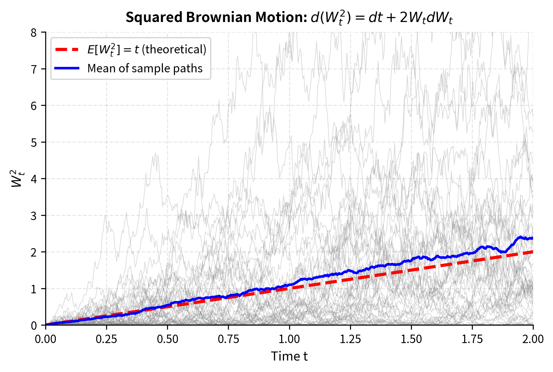
Example 1: Squared Brownian Motion
Consider where is standard Brownian motion. Here (the process is Brownian motion itself with and ). This simple example clearly demonstrates how Itô's Lemma differs from ordinary calculus.
Computing the partial derivatives:
where:
-
: the function being differentiated
-
: the stochastic process (Brownian motion)
Applying Itô's Lemma with and :
where:
-
: differential of the squared Brownian motion
-
: contribution from the Itô correction term
-
: contribution from the standard chain rule
Notice that the ordinary chain rule would give , missing the term entirely. The extra term comes from the Itô correction and reflects the fact that Brownian motion is constantly fluctuating. Even when , the squared process is increasing on average. This may seem counterintuitive at first, but it makes sense: when the Brownian motion passes through zero, it doesn't stay there. The constant oscillations around zero still contribute positive values to the squared process.
We can verify this result and gain further insight by integrating both sides:
where:
-
: terminal squared value of Brownian motion
-
: total time horizon (integral of the deterministic drift )
-
: stochastic integral term
-
: value of Brownian motion at time
Rearranging gives us an explicit formula for the stochastic integral:
where:
-
: stochastic integral of Brownian motion with respect to itself
-
: squared terminal value of Brownian motion
Compare this to ordinary calculus, where . The correction term appears because stochastic integrals behave differently from ordinary integrals. This example showcases how the Itô correction manifests in integral form.
Example 2: Log of Geometric Brownian Motion
This is the most important example for finance because it connects the geometric Brownian motion model of asset prices to the lognormal distribution. Suppose follows geometric Brownian motion:
where:
-
: asset price
-
: drift parameter
-
: volatility parameter
-
: Brownian increment
Let . We want to find the dynamics of the log-price, which will reveal important properties about the distribution of future prices. Computing derivatives with respect to :
where:
-
: natural logarithm function
-
: geometric Brownian motion process
Notice that the second derivative is negative, indicating that the logarithm function is concave. This concavity will cause the Itô correction to subtract from the drift rather than add to it.
Applying Itô's Lemma with and :
where:
-
: differential of the log-price process
-
: drift of the log-price
-
: volatility of the log-price
This is an important result. Even though follows geometric Brownian motion (a complicated multiplicative process with state-dependent coefficients), its logarithm follows simple arithmetic Brownian motion with constant drift and constant volatility . This transformation to additive dynamics makes GBM tractable.
Integrating from to :
where:
-
: asset prices at times and
-
: drift and volatility parameters
-
: Brownian motion value at
Since , we can immediately determine the distribution of log-returns:
where:
-
: log-return over the period
This proves that log-returns are normally distributed under the GBM model. Taking the exponential of both sides yields the explicit solution to the GBM SDE:
where:
-
: asset price at time
-
: initial asset price
-
: expected return parameter
-
: volatility parameter
-
: value of Brownian motion at time
The term is called the Itô drift correction. It explains why the expected log-return is less than the expected percentage return . This correction arises from the concavity of the logarithm function combined with the volatility of the underlying process. It has profound implications for portfolio theory and long-term wealth accumulation, as we shall see in later chapters.
Example 3: The Exponential Martingale
Consider . This exponential form appears frequently in risk-neutral pricing and change of measure arguments. The specific form of the exponent, with its term, is carefully chosen to produce a special property.
Let , or equivalently, .
Computing derivatives:
where:
-
: the function defining the martingale
-
: value of the exponential martingale
-
: volatility parameter
Applying Itô's Lemma (with , so , ):
where:
-
: change in the martingale process
-
: volatility term proportional to the process level
The process has zero drift! This means is a martingale, which is a process whose expected future value equals its current value. The careful choice of in the exponent exactly cancels the Itô correction that would otherwise appear from the convexity of the exponential function. This cancellation is not coincidental; it is precisely engineered to eliminate the drift.
This exponential martingale will be crucial when we study risk-neutral valuation in the next chapter. It provides the mathematical mechanism for changing from the real-world probability measure to the risk-neutral measure, which is essential for derivative pricing.
Example 4: Product of Two Itô Processes
Sometimes we need the dynamics of a product , for example when computing the dynamics of wealth or hedged portfolio value. The product rule for Itô processes differs from the ordinary product rule by an additional term:
where:
-
: differential of the product
-
: two Itô processes
-
: quadratic covariation term
The extra term has no analog in ordinary calculus. It arises from the cross-term in the Taylor expansion and survives because of the non-zero quadratic variation of Brownian motion.
Using the multiplication rules that encode the behavior of infinitesimal products:
-
(second-order in time, negligible)
-
(mixed term, order , negligible)
-
(quadratic variation of Brownian motion)
If and (driven by the same Brownian motion), then:
where:
- : diffusion coefficients of and
The full product rule becomes:
where:
-
: differential of the product process
-
: interaction term from covariance term in the drift represents the correlation between the two processes. When both processes are driven by the same Brownian motion and both have positive diffusion coefficients, this term adds to the drift of the product. This effect captures the idea that correlated random movements reinforce each other when considering the product.
Code Implementation
Let's implement simulations to verify our analytical results from Itô's Lemma.
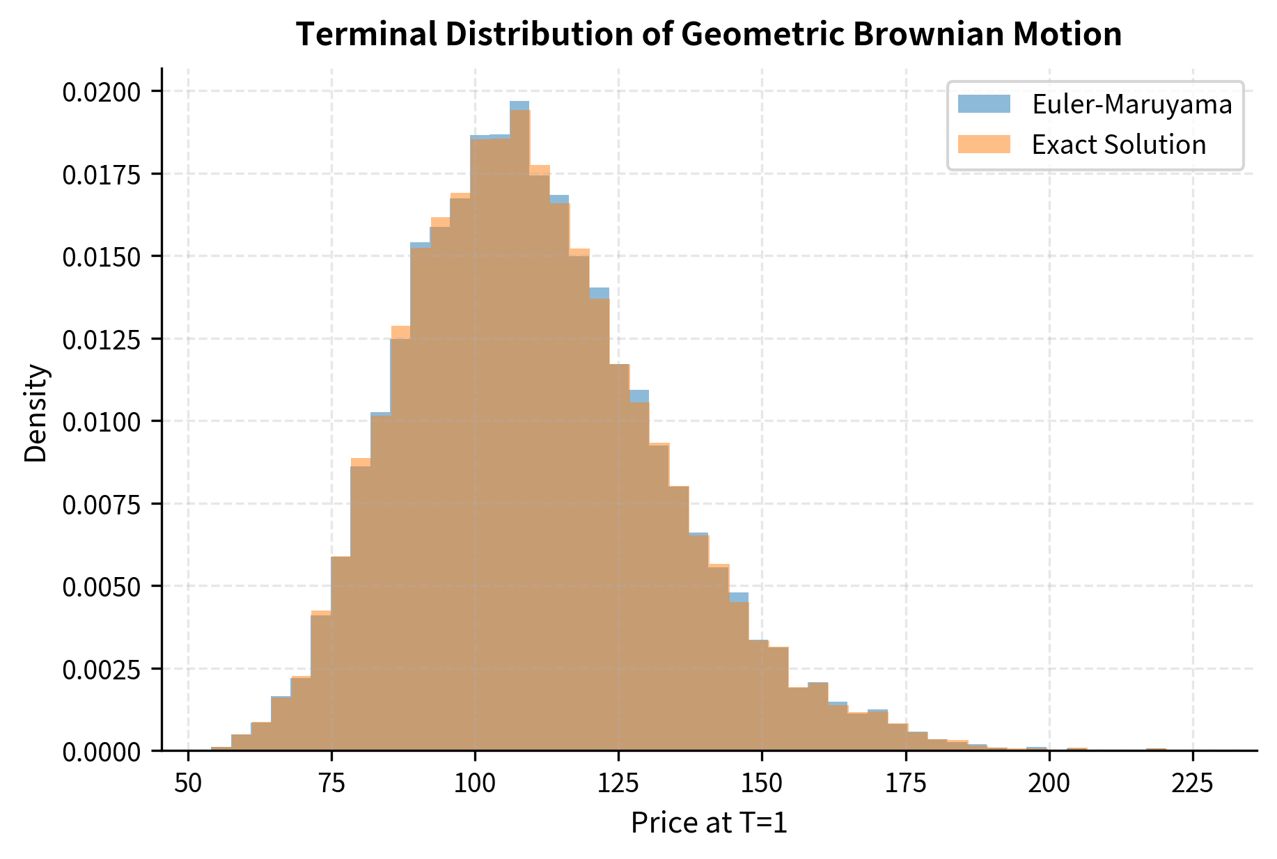
Verifying the GBM Solution
We derived that . Let's compare the Euler-Maruyama simulation with the exact solution.
The Euler-Maruyama approximation closely matches the exact solution, with small differences due to the discretization error.
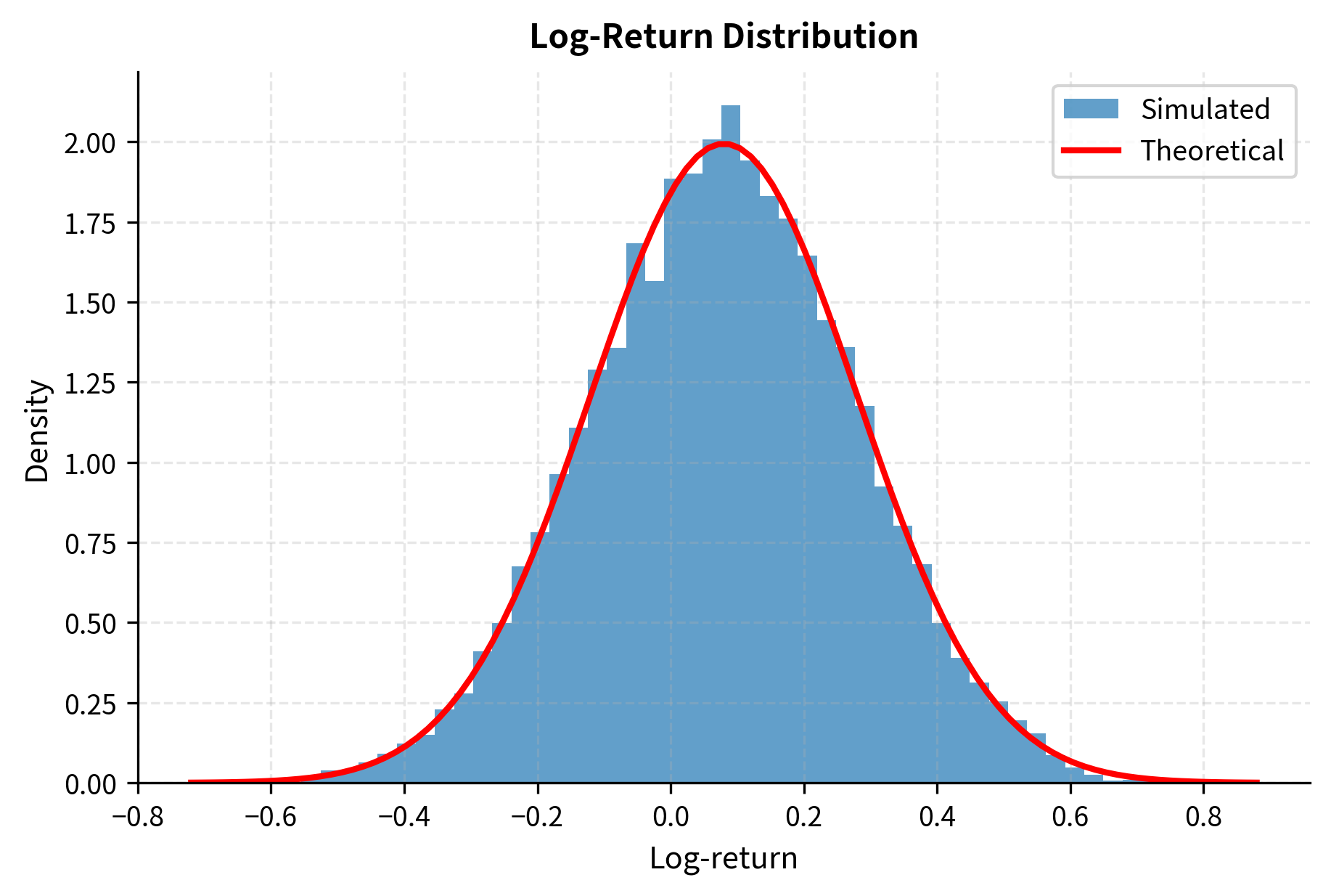
Verifying the Log-Return Distribution
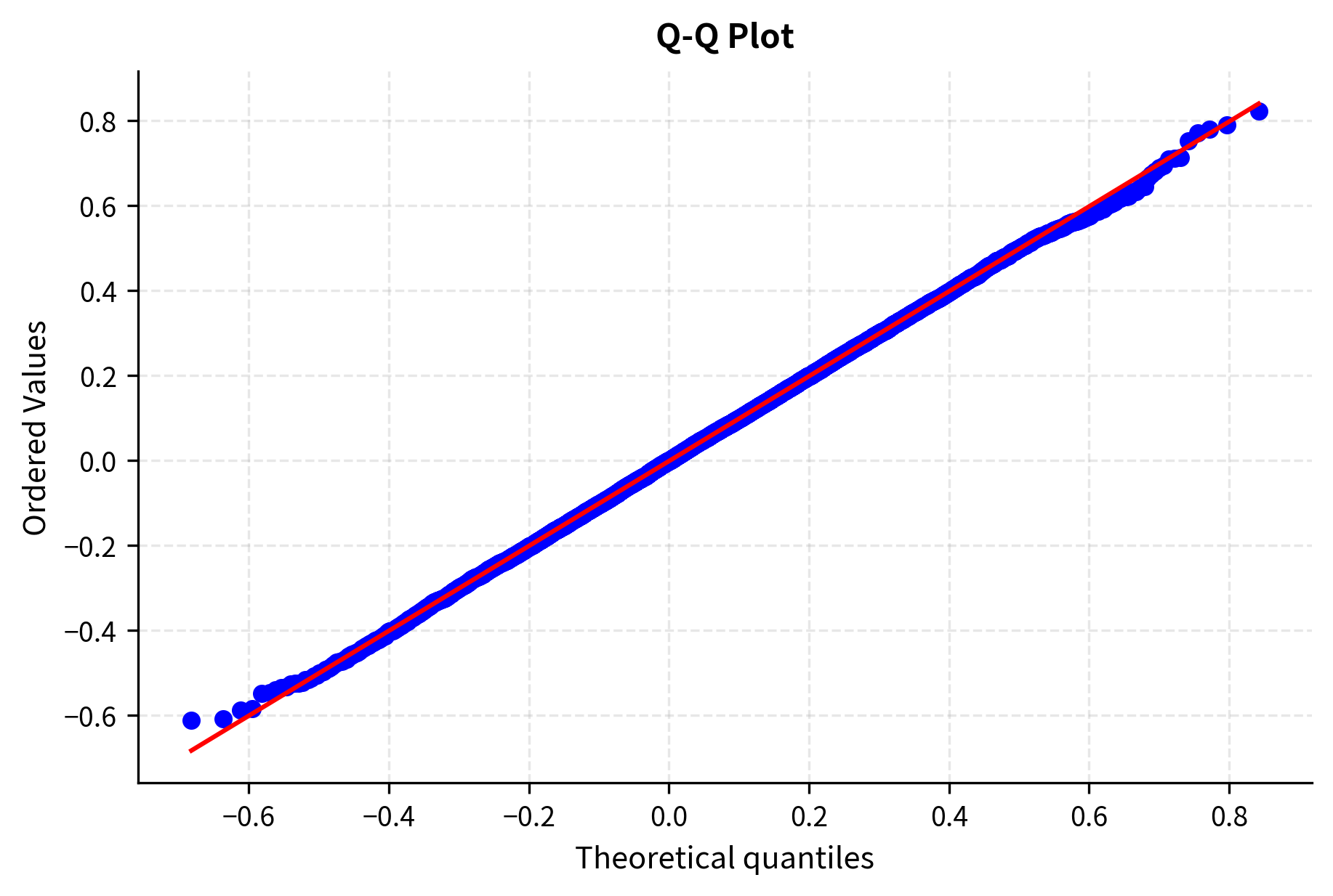
Itô's Lemma tells us that .
The simulated log-returns match the theoretical distribution predicted by Itô's Lemma, and the Shapiro-Wilk test confirms normality.
Visualizing the Itô Correction
The Itô correction has a significant impact, especially for high volatility. Let's visualize this.
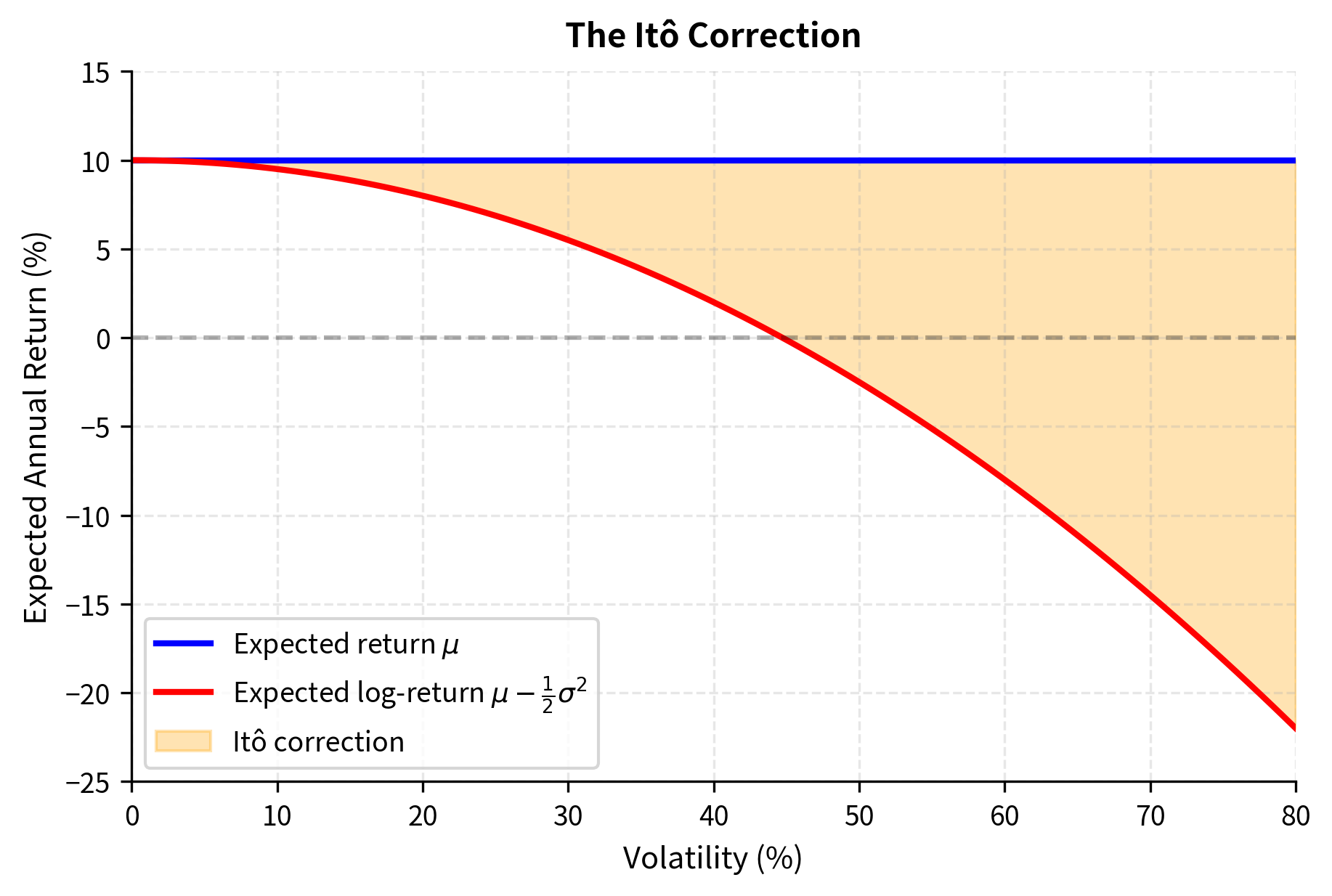
This graph illustrates why high-volatility assets can have positive expected returns but negative expected log-returns. For example, with and , the expected log-return is only . At , the expected log-return becomes negative despite the positive drift! This phenomenon has significant implications for long-term investing and helps explain why highly volatile assets can be poor long-term investments even when their expected single-period returns are positive.
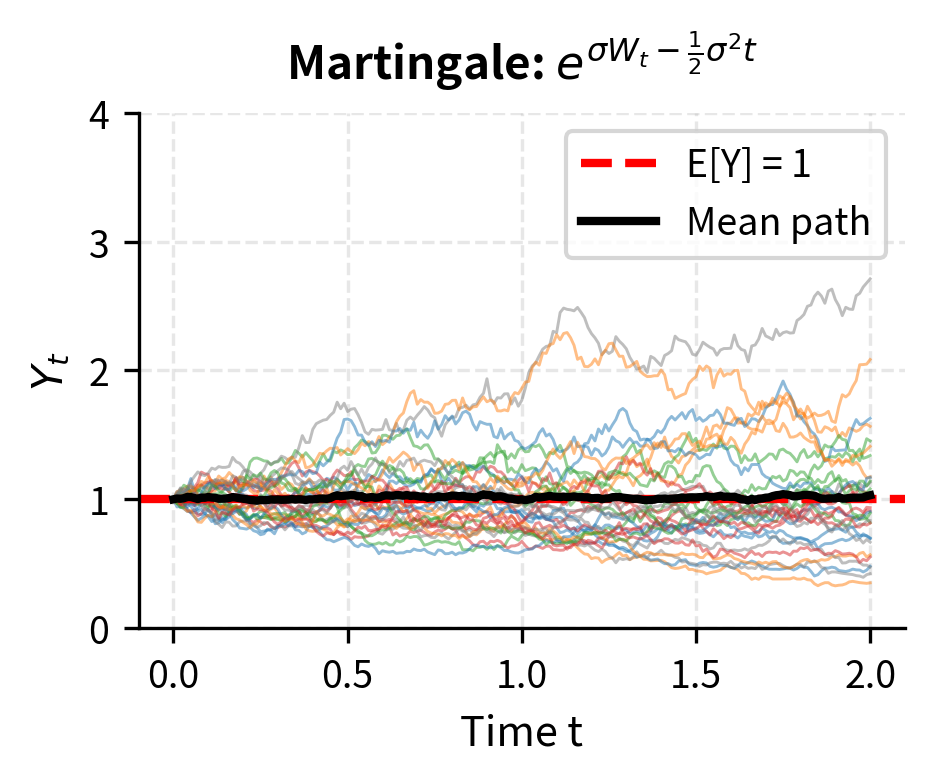
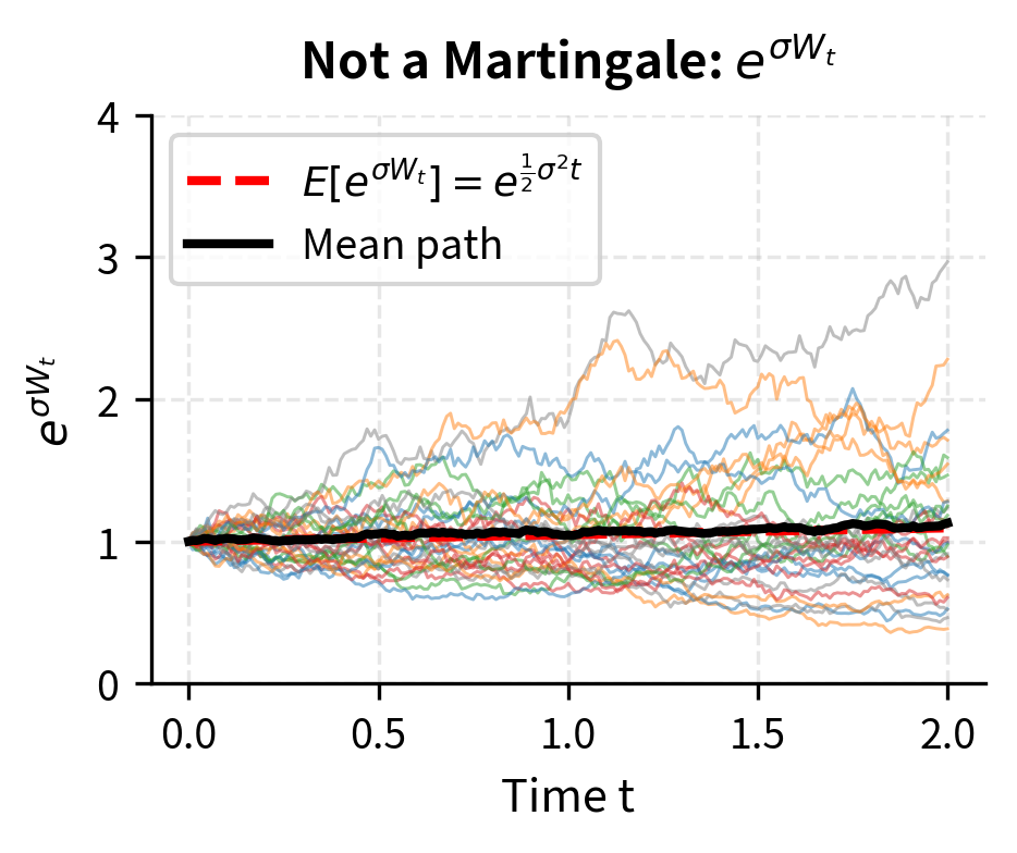
Verifying the Exponential Martingale
We showed that is a martingale. Let's verify that .
The exponential martingale with the correction has expected value 1, while the uncorrected version has expected value . This difference is precisely the Itô correction at work. The correction term in the exponent exactly compensates for the convexity of the exponential function, ensuring that the process has no drift.
Key Parameters
The key parameters used in the stochastic calculus simulations are:
-
S0: Initial asset price ($100)
-
mu: Drift rate (). Represents the expected annualized return.
-
sigma: Volatility (). Represents the annualized standard deviation of returns.
-
T: Time horizon in years.
-
n_steps: Number of discrete time steps (e.g., 252 for daily steps).
-
n_paths: Number of Monte Carlo paths simulated.
Multiple Correlated Brownian Motions
In practice, we often model multiple assets, each driven by its own source of randomness. This requires extending Itô's Lemma to handle multiple correlated Brownian motions. Understanding this extension is essential for portfolio analysis, multi-asset derivatives, and any application where the joint behavior of several random quantities matters.
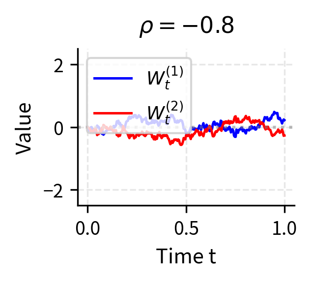
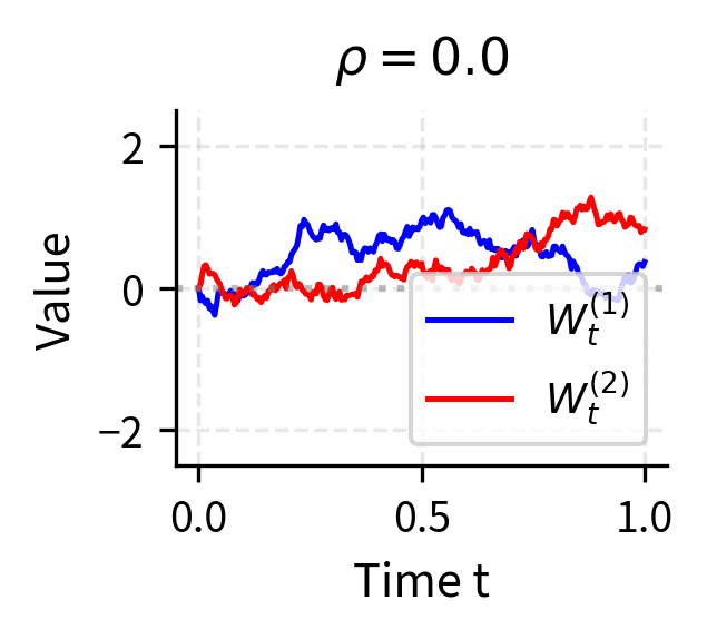
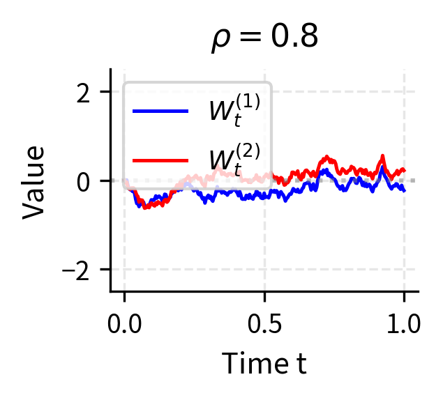
Correlated Brownian Motions
Suppose we have two Brownian motions and with correlation . This correlation captures the tendency of the two sources of randomness to move together. Their increments satisfy a relationship that generalizes the single-variable quadratic variation:
where:
- : correlation coefficient between the two Brownian motions
When , the two Brownian motions are identical; when , they move in exactly opposite directions; when , they are independent. Values between these extremes produce partial correlation.
The multiplication rules extend naturally to this setting:
-
(quadratic variation of the first Brownian motion)
-
(quadratic variation of the second Brownian motion)
-
(cross-variation capturing correlation)
Multidimensional Itô's Lemma
For a function where each follows an Itô process:
where:
-
: -th stochastic process
-
: drift and diffusion coefficients for process
Itô's Lemma generalizes to include all first-order terms and all second-order terms:
where:
-
: function of multiple stochastic processes and time
-
: -th state variable
-
: differential of the -th process
-
: covariance term, equal to
The double sum in the second-order terms captures all pairwise interactions between the stochastic processes. When , we get the standard Itô correction from each process's own quadratic variation. When , we get cross terms that depend on the correlation between the processes. This extension is essential for pricing options on multiple assets, modeling portfolio dynamics, and understanding correlation risk in complex financial instruments.
Limitations and Impact
Stochastic calculus provides a powerful framework, but its assumptions do not perfectly match real markets. This section examines model limitations and their impact on finance.
Limitations of Stochastic Calculus Models
While Itô's Lemma and the stochastic calculus framework provide powerful tools for modeling financial markets, they rest on assumptions that don't perfectly match real markets. Understanding these limitations helps you apply the models correctly and know when to use other methods.
Continuous paths assumption. Brownian motion has continuous paths, but real asset prices can jump discontinuously due to earnings announcements, central bank decisions, or market crashes. These sudden changes cannot be captured by a process with continuous sample paths. Jump-diffusion models, which combine continuous Brownian motion with discrete jumps, address this limitation but require more complex mathematics. The jump analog of Itô's Lemma involves integral terms over the jump distribution, significantly complicating both theory and computation. Flash crashes, like the May 2010 event where the Dow dropped nearly 1,000 points in minutes, cannot be captured by pure diffusion models and show that market prices sometimes move discontinuously.
Constant volatility assumption. The basic GBM model assumes constant volatility , but volatility clearly varies over time. Periods of market stress exhibit elevated volatility, while calm periods show subdued fluctuations. The implied volatility smile we observe in options markets directly contradicts the constant volatility assumption, as options with different strikes on the same underlying asset trade at prices implying different volatilities. Stochastic volatility models (like Heston) address this by making volatility itself follow an Itô process, but this significantly complicates the analysis and typically requires numerical methods for pricing.
Model risk and discretization. In practice, we simulate continuous-time models using discrete time steps because computers cannot handle truly continuous processes. The Euler-Maruyama method converges at rate , which is slower than typical numerical methods for ordinary differential equations. This slower convergence rate means that accurate simulation requires smaller time steps and more computation. For processes with mean-reversion or strong nonlinearity, more sophisticated discretization schemes (like Milstein or implicit methods) may be necessary for accuracy.
Impact on Quantitative Finance
Despite these limitations, Itô's Lemma fundamentally transformed quantitative finance by providing a rigorous mathematical framework for analyzing securities with random payoffs:
Derivatives pricing revolution. Itô's Lemma enabled the derivation of the Black-Scholes-Merton equation, which we'll cover in detail in the upcoming chapters. By applying Itô's Lemma to an option price as a function of the underlying asset, we can derive the partial differential equation that option prices must satisfy. This connection between SDEs and PDEs opened the door to modern derivatives pricing and created an entirely new industry of quantitative finance.
Risk-neutral valuation. The exponential martingale example foreshadows a deep connection: by choosing the right drift adjustment, we can transform a risky asset into a martingale. This is the foundation of risk-neutral pricing, which allows us to value derivatives without knowing the true drift of the underlying asset. Only the volatility matters for pricing. We'll explore this profound result in the next chapter on the no-arbitrage principle.
Unified framework for continuous-time finance. Stochastic calculus provides a common language for term structure models, credit models, and exotic derivatives. Whether modeling interest rate dynamics with the Vasicek or Cox-Ingersoll-Ross models, or pricing path-dependent options like Asian or barrier options, the same Itô calculus machinery applies. This unification allows techniques developed in one area to be transferred to others and provides a coherent intellectual framework for understanding diverse financial instruments.
Summary
This chapter introduced the mathematical framework of stochastic calculus, essential for modeling and pricing derivatives in continuous time.
Core concepts covered:
-
Stochastic differential equations (SDEs) describe how random processes evolve, with a drift component representing the expected trend and a diffusion component capturing random fluctuations.
-
The quadratic variation property is the key insight distinguishing stochastic from ordinary calculus. This means second-order terms in Brownian motion contribute to first-order changes in functions of the process.
-
Itô's Lemma extends the chain rule to stochastic processes:
where:
-
: differential of the function
-
: drift and diffusion coefficients of the underlying process
-
partial derivatives: sensitivity of to time and state
Key applications demonstrated:
-
The log of GBM follows simple Brownian motion:
-
The Itô correction explains why expected log-returns differ from expected simple returns
-
The exponential martingale has zero drift, foreshadowing risk-neutral pricing
With Itô's Lemma in hand, we're now equipped to tackle the central problems of derivatives pricing. In the next chapter, we'll introduce the no-arbitrage principle and risk-neutral valuation, which together with Itô's Lemma form the foundation for deriving the Black-Scholes-Merton equation.
Quiz
Ready to test your understanding? Take this quick quiz to reinforce what you've learned about Itô's Lemma and stochastic calculus.

Comments