

Master CDO mechanics, cash flow waterfalls, and correlation risk. Learn tranche valuation, the Gaussian copula model, and lessons from the 2008 crisis.
Choose your expertise level to adjust how many terms are explained. Beginners see more tooltips, experts see fewer to maintain reading flow. Hover over underlined terms for instant definitions.
Structured Credit Products (CDOs and Securitizations)
The securitization revolution transformed modern finance by converting pools of illiquid loans into tradable securities. At its core, securitization addresses a fundamental problem: banks originate loans that tie up capital for years or decades, limiting their ability to make new loans. By packaging these loans and selling them to investors, banks free up capital, distribute risk, and create new investment opportunities across the risk spectrum.
This chapter explores the mechanics of asset securitization and its most complex manifestation: the Collateralized Debt Obligation (CDO). We'll examine how pooling and tranching create securities with vastly different risk profiles from the same underlying assets, how cash flows cascade through the structure, and why correlation assumptions proved so dangerous in the 2008 financial crisis. Building on our understanding of credit default swaps from the previous chapter, you'll see how these instruments combine to create products that can either distribute risk efficiently or concentrate it catastrophically.
Asset Securitization Fundamentals
Securitization is the process of transforming a pool of illiquid assets, typically loans or receivables, into marketable securities. The technique emerged in the 1970s with mortgage-backed securities (MBS) and has since expanded to include auto loans, credit card receivables, student loans, and corporate debt.
The Securitization Process
The basic securitization structure involves several key participants. Understanding their interactions is essential to grasping how the structure works:
- Originator: A bank or financial institution that creates the underlying loans (mortgages, auto loans, etc.)
- Special Purpose Vehicle (SPV): A bankruptcy-remote entity created solely to hold the pooled assets
- Servicer: Collects payments from borrowers and distributes them to investors
- Investors: Purchase the securities backed by the asset pool
The SPV is critical to the structure, serving as the legal backbone that makes securitization work. By purchasing the assets from the originator, the SPV legally isolates them from the originator's bankruptcy risk. This isolation, known as "bankruptcy remoteness," is what transforms the credit quality of the underlying loans into something potentially superior to the originator's own creditworthiness. If the originating bank fails, investors still have claims on the underlying assets because those assets no longer belong to the bank. They belong to the SPV, which exists solely to hold and manage them. This legal separation is what allows a struggling bank to securitize high-quality mortgages and have those securities trade independently of the bank's own financial distress.

Why Securitize?
Securitization offers benefits to multiple parties:
- Originators free up capital, earn origination and servicing fees, and transfer credit risk off their balance sheets
- Investors gain access to asset classes previously unavailable to them, with customizable risk-return profiles
- Borrowers benefit from increased credit availability as banks can lend more when they can sell loans
- Markets achieve more efficient risk distribution as credit risk flows to those best able to bear it
The transformation from illiquid loans to tradable securities also creates price transparency and liquidity, enabling more efficient capital allocation across the economy.
Collateralized Debt Obligations
A Collateralized Debt Obligation (CDO) takes securitization a step further by pooling debt instruments, such as corporate bonds, loans, mortgage-backed securities, or even other CDOs, and issuing securities in multiple tranches with different risk and return characteristics.
From the French word for "slice," a tranche is a portion of a securitized product with specific risk, return, and maturity characteristics. Tranches are ordered by seniority, determining the order in which they receive payments and absorb losses.
Types of CDOs
CDOs come in several varieties based on their underlying assets and structure:
-
CLOs (Collateralized Loan Obligations): Backed by leveraged loans to corporations
-
CBOs (Collateralized Bond Obligations): Backed by high-yield corporate bonds
-
Structured Finance CDOs: Backed by other asset-backed securities, including MBS
-
Synthetic CDOs: Use credit default swaps rather than physical assets to gain credit exposure
The distinction between cash CDOs and synthetic CDOs is fundamental. Cash CDOs hold actual debt instruments and distribute the cash flows from those instruments. Synthetic CDOs, as we discussed in the previous chapter on credit default swaps, use CDS contracts to create credit exposure without owning the underlying bonds.
CDO Tranching Structure
The defining feature of a CDO is its capital structure, which divides the pool's risk and return among tranches with different levels of seniority. This tranching mechanism is the financial engineering that allows a single pool of assets to simultaneously satisfy conservative investors seeking stable returns and aggressive investors seeking higher yields. The same underlying loans, through clever structuring, become multiple distinct securities.


The key parameters defining each tranche are:
- Attachment point: The cumulative loss level at which the tranche begins absorbing losses
- Detachment point: The loss level at which the tranche is completely wiped out
- Thickness: The difference between detachment and attachment points
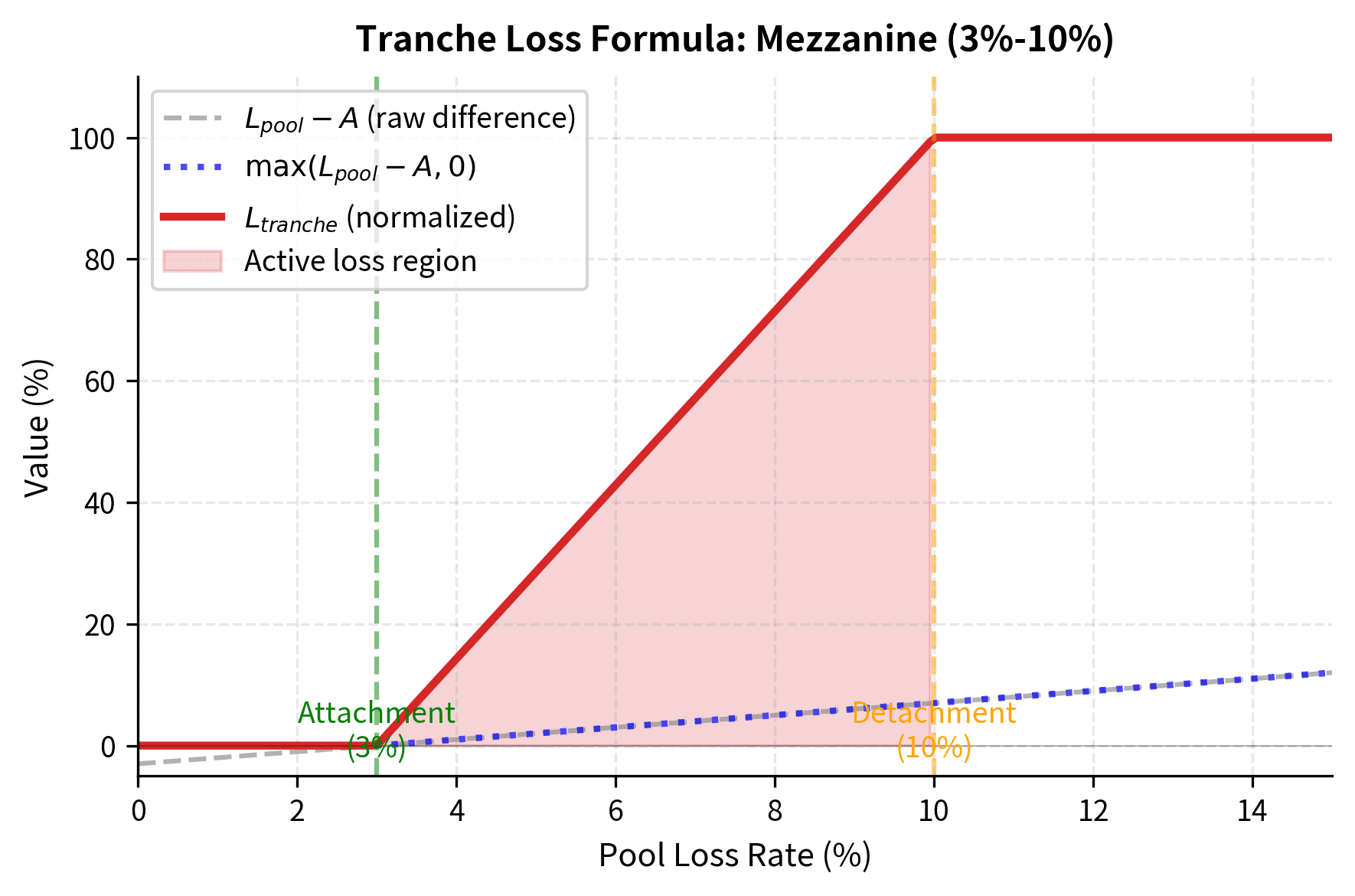
To understand how these parameters work together, consider a mezzanine tranche with a 3% attachment point and 10% detachment point, giving it a 7% thickness. This tranche sits in the middle of the capital structure, protected by the equity tranche below it but subordinate to the senior tranche above. The tranche absorbs no losses whatsoever until the total pool losses exceed 3%. Once pool losses cross that 3% threshold, the mezzanine tranche begins absorbing all marginal losses. It continues absorbing every additional dollar of loss until pool losses reach 10%, at which point the mezzanine tranche is completely exhausted and the senior tranche begins to suffer.
Mathematically, we can express the tranche loss percentage as:
where:
- : percentage loss allocated to the tranche
- : cumulative percentage loss of the underlying collateral pool
- : attachment point (e.g., 3%), the threshold where the tranche begins to lose value
- : detachment point (e.g., 10%), the threshold where the tranche is wiped out
- : tranche thickness
This formula captures the layered loss allocation through nested minimum and maximum functions. Let's break down each component to understand the mechanics:
The innermost expression, , calculates the amount by which pool losses exceed the attachment point. If the pool has lost 7% and the attachment point is 3%, this difference equals 4%, representing the losses that have "reached" this tranche.
The maximum function, , ensures the tranche loses nothing if pool losses remain below the attachment point . When pool losses are only 2% against a 3% attachment point, the difference is negative, but the maximum function returns zero because the tranche is still fully protected by the subordination below it.
The minimum function, , caps the loss at the tranche thickness (), so the tranche cannot lose more than its total notional value. Once pool losses exceed the detachment point, this tranche has nothing more to lose; the excess losses pass through to the next senior tranche.
Finally, the division by converts the dollar loss into a percentage of the tranche's notional, normalizing the result to a value between 0 and 1.
This "call spread" payoff structure means the tranche behaves like an option on the pool losses. Specifically, owning a tranche is economically equivalent to being long a call option on pool losses struck at the attachment point and short a call option struck at the detachment point. This options-based perspective proves valuable when we consider hedging strategies and the relationship between tranche pricing and correlation.
Cash Flow Waterfall
The waterfall structure determines how cash flows from the underlying assets are distributed among tranches. This mechanism is what creates the different risk profiles, ensuring that senior tranches receive their promised payments before junior tranches see any return.
Priority of Payments
In a typical cash CDO, cash flows follow a strict priority known as the waterfall. The term "waterfall" evokes the image of water flowing down a series of pools: the top pool must fill completely before any water spills to the next level, and so on down the structure. Similarly, each category of payment must be satisfied in full before the next category receives anything:
- Trustee and administrative fees
- Senior tranche interest
- Mezzanine tranche interest
- Senior tranche principal (if coverage tests fail)
- Mezzanine tranche principal (if coverage tests fail)
- Equity tranche (residual cash flows)
This priority structure explains why senior tranches can achieve AAA ratings even when the underlying loans are far from risk-free. The senior tranche receives payment first, and it only suffers losses after all subordinate tranches have been completely wiped out. In essence, the equity and mezzanine tranches serve as a buffer, absorbing losses that would otherwise reach senior investors.
Let's implement a simplified waterfall model to see how this works in practice:
Now let's create a CDO and see how it distributes cash flows under different loss scenarios:


This analysis reveals the leverage embedded in lower tranches. At 5% pool losses, the equity tranche is wiped out (100% loss), the mezzanine has lost 28.6% of its value, while the senior tranche remains untouched. The equity tranche, representing only 3% of the capital structure, absorbs the entire impact of moderate losses. This leverage cuts both ways: in good times, the equity tranche captures all excess returns, but in bad times, it bears concentrated losses that far exceed the pool's overall loss rate.

Credit Risk Distribution and Correlation
The critical insight about CDO tranches is that their risk depends not just on the probability of individual defaults, but on the default correlation of defaults across the pool. This correlation effect is what made CDO valuation so challenging and what contributed to the 2008 crisis. Understanding correlation is essential because it determines whether losses will be spread evenly across scenarios or concentrated in catastrophic tail events.
Default Correlation
Consider two extreme scenarios for a pool of 100 identical loans, each with a 5% probability of default. These extremes illustrate why correlation matters so profoundly for tranche valuation:
- Zero correlation: Defaults occur independently. By the law of large numbers, we expect very close to 5 defaults in virtually every scenario. The variance of losses is low, and extreme outcomes are rare.
- Perfect correlation: All loans default together or none do. There's a 5% chance of total loss and 95% chance of zero loss. The average loss is still 5%, but the distribution is bimodal with no middle outcomes.
In reality, loans are somewhere between these extremes. They share exposure to common economic factors such as interest rates, unemployment, and GDP growth that create positive default correlation. When the economy weakens, multiple borrowers struggle simultaneously, causing defaults to cluster rather than occur randomly.
The model above implements the one-factor Gaussian copula approach, which became the industry standard for CDO valuation. The fundamental idea is elegant: rather than modeling the complex dependencies between thousands of individual borrowers, we assume that all correlation arises from exposure to a single common factor representing the overall state of the economy.
Each asset's latent value is driven by a combination of systematic and idiosyncratic risk:
where:
- : latent variable representing the creditworthiness of asset
- : asset correlation coefficient ()
- : systematic market factor affecting all assets,
- : idiosyncratic factor specific to asset ,
The coefficients and may seem like arbitrary choices, but they are precisely calibrated to preserve unit variance in the latent variable while achieving the desired correlation structure. Since and are independent standard normal variables, we can demonstrate this property step-by-step:
This unit variance property ensures that is itself a standard normal variable, which simplifies the default threshold calculation considerably.
Asset defaults if its value falls below a specific threshold determined by its default probability:
where:
- : unconditional probability of default for the asset
- : inverse cumulative distribution function of the standard normal distribution
Since follows a standard normal distribution, the probability of observing a value below is exactly , ensuring the model matches the individual default probability regardless of the correlation parameter.
Intuitively, represents the firm's asset value or creditworthiness. When falls below the threshold, the firm's assets are insufficient to meet its obligations, triggering default. The correlation parameter controls how much the asset values move together. When is high, the systematic factor dominates, and defaults cluster because a bad draw for pushes all firms toward the default threshold simultaneously. When is low, the idiosyncratic factors dominate, and defaults occur more independently.


Correlation's Asymmetric Impact on Tranches
The correlation effect impacts tranches differently, and this asymmetry is perhaps the most important insight for understanding CDO risk. Higher correlation makes extreme outcomes more likely at both ends of the distribution: both zero defaults and catastrophic defaults become more probable, while moderate outcomes become less likely.
This table reveals a crucial insight that is central to understanding CDO risk: correlation impacts senior and equity tranches in opposite directions. As correlation increases:
- The equity tranche becomes less risky because clustering defaults means more scenarios with zero or few defaults. With high correlation, there are many scenarios where the economy performs well and almost no one defaults, allowing the equity tranche to survive unscathed.
- The senior tranche becomes more risky because the tail of extreme losses gets fatter. Although the senior tranche still survives in most scenarios, the probability of catastrophic losses (those exceeding 10% of the pool) increases substantially.
- The mezzanine tranche is relatively stable across correlations, sitting in a middle ground where the opposing effects roughly cancel out.
This asymmetry has profound implications for hedging and valuation. An investor who is long the equity tranche and short the senior tranche has significant exposure to correlation: if correlation increases, the position gains value as equity risk falls and senior risk rises. Conversely, the opposite position loses value. This correlation exposure made hedging CDO portfolios extremely difficult during the 2008 crisis, when realized correlations spiked far beyond historical norms.


Valuation Approaches
Valuing CDO tranches requires estimating the expected losses and timing of cash flows. The standard approaches fall into two categories: actuarial methods based on expected loss, and risk-neutral valuation using credit derivatives. The challenge lies in calibrating models to observable market prices while maintaining consistency across the capital structure.
Base Correlation
Given the difficulty of directly calibrating individual asset correlations, we use base correlation, which is the implied correlation that, when plugged into the Gaussian copula model, matches the market price of a tranche. Base correlation emerged as a practical solution to a fundamental problem: if you calibrate separate correlations to each tranche independently, you get different values, which makes it impossible to consistently price non-standard tranches or interpolate between market quotes.
The implied correlation for an equity tranche (0% attachment to X% detachment) that matches its market price. Unlike "compound correlation" which can give different values for different tranches on the same structure, base correlation provides a consistent framework for interpolating between standard tranches.
Base correlation is analogous to implied volatility in options pricing. Just as options traders quote prices in terms of implied volatility rather than dollar amounts, credit traders quote CDO tranches in terms of base correlation. It is a quoting convention that captures market views about the distribution of losses, converting complex distributional assumptions into a single, comparable number. When base correlation for a 10% equity tranche increases, it signals that the market expects a fatter-tailed loss distribution with more probability mass in extreme scenarios.

The upward-sloping base correlation curve, analogous to the volatility smile we'll explore in Part III, indicates that the market expects loss distributions with fatter tails than a single-correlation Gaussian copula would produce. Senior tranches require higher implied correlations to match their market prices, suggesting investors demand compensation for extreme scenarios that the base model underestimates. This "correlation smile" became a key indicator of market stress, widening dramatically during periods of credit turmoil.
Synthetic CDOs and Credit Indices
Synthetic CDOs, introduced after the credit default swap market matured, use CDS contracts instead of physical bonds to create credit exposure. They became the dominant CDO structure due to lower execution costs and greater flexibility.
CDX and iTraxx Indices
Standardized credit indices made synthetic CDO trading more liquid:
- CDX (North America): 125 investment-grade names in CDX.IG, 100 high-yield names in CDX.HY
- iTraxx (Europe and Asia): Similar structures for European and Asian credits
These indices and their tranches trade with standardized terms, enabling more transparent price discovery than bespoke CDO structures.

The equity tranche trades with an upfront payment plus a fixed 500 bps running spread, while other tranches trade on a running spread basis. This convention reflects the high expected losses in the equity tranche, making a pure running spread impractical.
Worked Example: Analyzing a $500M CDO
Let's work through a complete example of a cash CDO backed by 100 corporate loans.
The simulation results quantify the risk segmentation. The Equity tranche, while offering potential upside, faces a high probability of total loss (approx. 60%). In contrast, the Senior tranche remains untouched in the vast majority of scenarios, protected by the subordination of the lower tranches.


Limitations and Historical Lessons
The 2008 financial crisis exposed fundamental weaknesses in structured credit markets. Understanding these failures is essential.
Model Risk and the Gaussian Copula
The Gaussian copula model, while mathematically elegant, made critical simplifying assumptions that proved dangerously wrong. The model assumes that correlation is constant across market regimes and that the relationship between asset values follows a Gaussian distribution. In reality, correlations spike during crises, exactly when they matter most. Assets that appeared uncorrelated during normal markets suddenly moved together as systemic stress propagated through interconnected financial institutions.
The model also struggles with "wrong-way risk": situations where the probability of default increases precisely when the value of recovery is lowest. Mortgage defaults, for example, correlate strongly with falling house prices, meaning both the frequency and severity of losses increase simultaneously. A single correlation parameter cannot capture these dynamics.
David Li, whose 2000 paper introduced the Gaussian copula to credit derivatives, later acknowledged its limitations. The formula became a tool of regulatory arbitrage: banks could use it to justify holding less capital against super-senior tranches rated AAA, even when those tranches were backed by increasingly risky subprime mortgages.
Rating Agency Failures
Credit rating agencies applied the same letter grades to CDO tranches that they used for corporate bonds, despite fundamental differences in the underlying risk. An AAA-rated corporate bond and an AAA-rated CDO super-senior tranche had the same five-year expected loss rate by construction, but vastly different risk profiles:
- Corporate bonds have diversified business risk with decades of historical default data
- CDO tranches had concentrated exposure to correlation assumptions with limited performance history
- CDO tranches exhibited "cliff risk": they could go from fully performing to severely impaired with small changes in underlying losses
The agencies also faced severe conflicts of interest, earning substantial fees from the banks structuring CDOs while rating them. When subprime mortgage performance deteriorated in 2007, mass downgrades of CDO tranches destroyed investor confidence and accelerated the crisis.
Complexity and Opacity
CDO-squared (CDO²) and CDO-cubed structures, which are CDOs backed by tranches of other CDOs, amplified model risk exponentially. The number of underlying loans could exceed 100,000, making due diligence effectively impossible. A single CDO² tranche might have exposure to thousands of individual mortgages across dozens of states, each with different underwriting standards and house price dynamics.
This complexity created asymmetric information between structurers and investors. Banks packaging these securities had access to loan-level data and sophisticated models; many investors relied entirely on credit ratings and offering documents. When the market turned, this information asymmetry contributed to a complete breakdown in trading liquidity.
Regulatory Response
Post-crisis reforms addressed several structural issues:
- Risk retention rules require originators to keep "skin in the game" by retaining at least 5% of securitized assets
- Enhanced disclosure mandates loan-level data availability for investors
- Higher capital charges make it more expensive for banks to hold securitized positions
- Simpler structures are encouraged through regulatory preference
The market for new CDOs collapsed after 2008 and has only partially recovered, with CLOs (backed by leveraged loans) becoming the dominant structure. Synthetic CDO activity remains limited and concentrated among sophisticated investors.
Credit Enhancement Mechanisms
Beyond tranching, CDO structures employ various credit enhancement mechanisms to improve tranche ratings and attract investors. These mechanisms provide additional protection to senior investors, helping to justify higher credit ratings and lower required yields:
Overcollateralization (OC) requires the collateral pool value to exceed the par value of issued tranches. If a CDO issues \1 billion in assets, the \$50 million difference provides a cushion against losses. This excess collateral absorbs initial losses before any tranche is impacted, providing an additional layer of protection beyond the subordination structure.
Subordination uses the existence of lower tranches as credit enhancement for higher tranches. The equity and mezzanine tranches provide credit support to the senior tranche by absorbing first losses. From the perspective of a senior investor, the junior tranches function as a deductible: losses must exhaust all junior capital before touching the senior tranche.
Reserve accounts hold cash to cover potential shortfalls in interest or principal payments. These accounts are typically funded from excess spread in early periods, building up a cushion of liquid assets that can bridge temporary payment gaps without triggering defaults to investors.
Coverage tests trigger mandatory principal paydowns if collateral quality deteriorates beyond specified thresholds. These tests act as circuit breakers, redirecting cash flows to protect senior investors when warning signs emerge. The OC_Ratio is a primary metric used in these tests, measuring the buffer of performing assets relative to outstanding liabilities:
where:
- OC_Ratio: ratio measuring the buffer of assets over liabilities
- Par_Value_of_Collateral: total face value of performing assets in the pool
- Senior_Notional: outstanding principal of the senior tranche
- Subordinate_Notional: outstanding principal of the relevant subordinate tranches
When this ratio falls below a predetermined trigger level, the structure automatically diverts cash flows from junior tranches to pay down senior principal. This mechanism accelerates the deleveraging of the structure, reducing senior exposure even as collateral quality deteriorates. The trigger levels are set to provide early warning: they trip before actual losses would reach the senior tranche, giving the structure time to de-risk.

When coverage tests fail, cash that would otherwise flow to equity or mezzanine tranches is redirected to pay down senior principal, protecting senior investors but accelerating losses for subordinate holders.
Summary
Structured credit products represent both financial innovation and financial engineering's potential for harm when misapplied. The key concepts from this chapter include:
Securitization mechanics transform illiquid assets into tradable securities through SPVs, providing capital relief for originators and investment opportunities for a wider investor base. The legal isolation of assets from originator bankruptcy risk is fundamental to the structure.
Tranching divides credit risk into slices with different attachment and detachment points. Senior tranches have priority claims and lower yields; equity tranches absorb first losses but capture excess spread. This creates securities with vastly different risk profiles from identical underlying assets.
Default correlation determines how losses cluster and is the critical variable in CDO valuation. Higher correlation reduces equity tranche risk (more scenarios with zero losses) but increases senior tranche risk (fatter tails). The Gaussian copula model's single correlation parameter proved inadequate for capturing real-world dynamics.
Cash flow waterfalls govern payment priority, with coverage tests triggering protective cash diversions when collateral quality deteriorates. Understanding the waterfall mechanics is essential for analyzing tranche behavior under stress scenarios.
Model risk was dramatically underestimated before 2008. The combination of complex structures, optimistic correlation assumptions, conflicted rating agencies, and opacity created a system primed for catastrophic failure. Post-crisis reforms emphasize simpler structures, better disclosure, and alignment of incentives through risk retention.
These instruments remain important in modern finance, particularly CLOs in the leveraged loan market. The lessons from their failures inform how we approach correlation modeling, stress testing, and the limits of financial engineering more broadly. As we move to convertible bonds in the next chapter, we'll see another form of structured security, one combining equity and debt features rather than slicing credit risk.
Quiz
Ready to test your understanding? Take this quick quiz to reinforce what you've learned about structured credit products and CDO mechanics.

Comments