

Learn interest rate swap fundamentals: cash flow mechanics, day count conventions, LIBOR to SOFR transition, hedging strategies, and market structure.
Choose your expertise level to adjust how many terms are explained. Beginners see more tooltips, experts see fewer to maintain reading flow. Hover over underlined terms for instant definitions.
Interest Rate Swaps - Fundamentals
Interest rate swaps are among the most widely traded financial instruments in the world, with notional amounts outstanding exceeding hundreds of trillions of dollars. At their core, swaps allow two parties to exchange streams of cash flows, typically transforming fixed-rate obligations into floating-rate ones or vice versa. This simple mechanism unlocked an enormous range of applications. Corporations can hedge their exposure to interest rate movements, banks can manage the duration mismatch between their assets and liabilities, and investors can express views on the future path of interest rates without buying or selling the underlying bonds.
The swap market emerged in the early 1980s when companies discovered they could reduce borrowing costs by exploiting their comparative advantages in different credit markets. A company with strong credit might borrow cheaply at a fixed rate, while another might have better access to floating-rate financing. By exchanging their interest payments, both could end up better off than if they had borrowed directly in their preferred market. This insight transformed corporate finance and risk management, creating a market that now dwarfs the underlying bond markets in notional terms.
Unlike the exchange-traded futures and options we covered earlier, swaps are over-the-counter (OTC) derivatives. This means they are privately negotiated contracts between two counterparties, offering flexibility in terms, notional amounts, and payment schedules that standardized exchange products cannot provide. However, this flexibility comes with counterparty credit risk, since each party depends on the other to honor their obligations throughout the life of the swap, which can extend for decades.
The Plain-Vanilla Interest Rate Swap
The most common type of interest rate swap is the plain-vanilla swap, where one party pays a fixed interest rate while receiving a floating rate tied to a reference index. Despite the name suggesting something simple, understanding the mechanics requires careful attention to several components. The "vanilla" designation indicates standardization rather than simplicity: these swaps follow well-established market conventions that have evolved over decades of trading, making them the benchmark against which all other swap structures are measured.
Swap Structure and Cash Flow Mechanics
In a plain-vanilla interest rate swap, two parties agree to exchange interest payments on a specified notional principal amount for a defined period. The key insight, and one that distinguishes swaps from loans or bonds, is that the notional principal itself is never exchanged. It serves only as the basis for calculating interest payments. This feature makes swaps fundamentally different from debt instruments: there is no transfer of capital at inception, no repayment at maturity, and no credit extended in the traditional sense. Instead, the parties are simply agreeing to exchange streams of payments calculated on a hypothetical principal amount.
The notional principal is the hypothetical amount used to calculate swap payments. Unlike a loan, this amount is never transferred between parties. It simply determines the size of the interest payments being exchanged.
Consider a swap with a notional principal of \$100 million. The fixed-rate payer agrees to pay, say, 4% per year on this notional, while receiving floating-rate payments based on a reference rate. If the floating rate happens to be 3.5% for a particular period, the fixed-rate payer pays $4 million annually while receiving $3.5 million. Rather than making gross payments in both directions, parties typically settle the net difference: the fixed-rate payer would pay $500,000 to the floating-rate payer. This netting convention reduces operational complexity and, more importantly, reduces the credit exposure between counterparties since only the smaller net amount changes hands.
Understanding the essential parameters of a swap provides the foundation for all subsequent analysis. Each parameter affects either the timing of cash flows, their magnitude, or both:
- Notional principal: The amount on which interest calculations are based. Common sizes range from $10 million to billions of dollars. The notional determines the scale of all payments, so a 1 basis point movement in rates has ten times the dollar impact on a $100 million notional compared to a $10 million notional.
- Trade date: When the parties agree to the swap terms. This is the date when economic exposure begins, even though cash flows may not start immediately.
- Effective date: When interest begins accruing, typically two business days after the trade date. This standard settlement convention, known as "T+2," allows time for documentation and operational processing.
- Maturity date: When the swap terminates and final payments are exchanged. Swap maturities can range from a few months to 30 years or more.
- Fixed rate: The predetermined rate paid by the fixed-rate payer, also called the swap rate. This rate is set at inception to make the swap's initial value close to zero, meaning neither party pays the other to enter the contract.
- Floating rate index: The reference rate that determines floating payments, historically LIBOR, now increasingly SOFR. The choice of index affects both the level and volatility of floating payments.
- Payment frequency: How often payments are exchanged, which may differ between the fixed and floating legs. Mismatched frequencies create periods where one leg pays and the other does not.
- Day count convention: The method for calculating the fraction of a year for each payment period. Different conventions can result in materially different payment amounts for the same rate.
The Fixed Leg
The fixed leg of a swap involves payments at a predetermined rate that remains constant throughout the life of the swap. The fixed-rate payer knows exactly what their payments will be from the outset, making this leg straightforward to calculate. This certainty is precisely why many hedgers prefer to pay fixed: they can budget for known interest costs regardless of how market rates evolve. The fixed leg transforms uncertainty into predictability, which has significant value for corporate treasurers and financial planners.
The calculation of fixed payments follows a straightforward formula that incorporates both the agreed rate and the time period for which interest accrues. The fixed payment for each period is:
where:
- : the principal amount used as the basis for calculations
- Fixed Rate: the predetermined interest rate agreed upon at inception
- Days in Period: number of days in the specific accrual period
- Days in Year: number of days in a year according to the day count convention (e.g., 360)
The formula reveals the modular nature of interest calculations: the notional scales the payment size, the fixed rate determines the annualized percentage, and the day count fraction adjusts for the specific time period. This structure allows us to compare rates across different payment frequencies and day count conventions by normalizing everything to an annual basis.
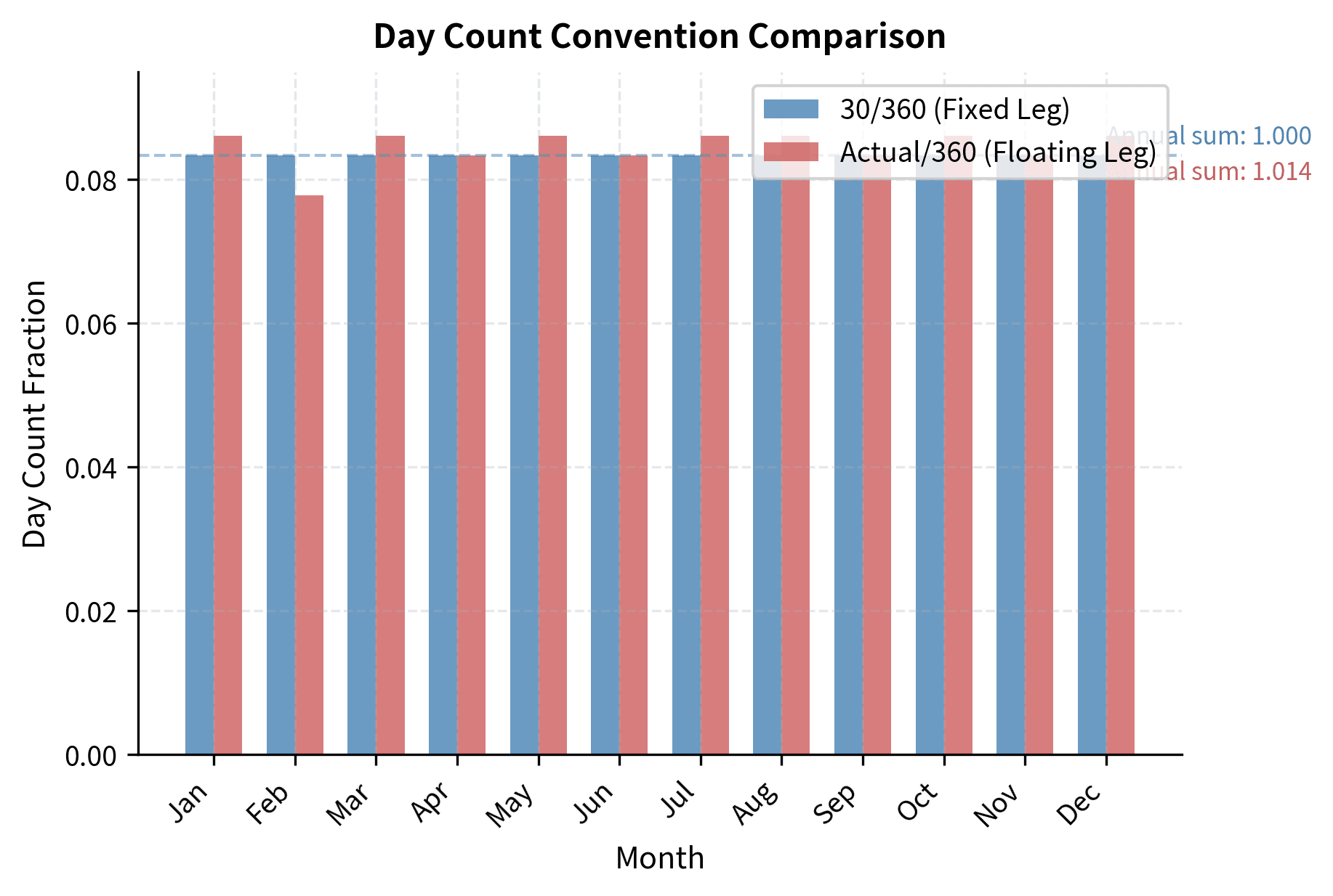
The day count convention determines how we measure the period length. For U.S. dollar swaps, the fixed leg typically uses the 30/360 convention, which assumes each month has 30 days and each year has 360 days. This simplifies calculations and standardizes payments across different months. Under this convention, February is treated as having 30 days rather than 28 or 29, and months with 31 days are shortened to 30. While this may seem arbitrary, the convention evolved because it makes payment amounts more predictable and easier to calculate by hand, which mattered greatly before computers became ubiquitous.
Under the 30/360 convention, a semi-annual payment on a \$100 million notional with a 4% fixed rate would be calculated as follows. Since six months equals 180 days under this convention, and the year contains 360 days, the fraction of the year is exactly 0.5:
This payment would occur every six months throughout the life of the swap, providing the fixed-rate payer with complete certainty about their future obligations.
The Floating Leg
The floating leg involves payments that reset periodically based on a reference interest rate. This creates uncertainty about future payments, which is precisely what makes swaps useful for hedging and speculation. While the fixed-rate payer knows all their payments at inception, the floating-rate payer only knows each payment shortly before it comes due. This asymmetry of information reflects the fundamental difference between the two legs: one provides certainty, the other provides market exposure.
The floating payment calculation mirrors the fixed leg structure but substitutes the observed reference rate for the predetermined fixed rate. The floating payment for each period is:
where:
- : the value of the reference index (e.g., SOFR) for the period
- : the principal amount (same as fixed leg)
- Days in Period: actual number of days in the accrual period
- Days in Year: typically 360 for floating legs (Actual/360 convention)
The parallel structure between fixed and floating payment formulas is intentional and important. Both calculations follow the same logic: multiply the notional by a rate and by a time fraction. This structural similarity allows for clean netting of payments and straightforward comparison of the two legs.
For floating legs, the day count convention is typically Actual/360, meaning the actual number of days in the period is divided by 360. This difference in day count conventions between fixed and floating legs is a common source of confusion but reflects market conventions that evolved over decades. The Actual/360 convention means that a 91-day quarter accrues slightly more than one-quarter of annual interest (91/360 = 25.28% rather than 25%), while the 30/360 convention would treat the same quarter as exactly 90/360 = 25%. Over a full year, these differences can result in the floating leg paying slightly more total days of interest than the fixed leg, creating a small systematic bias that market participants account for in pricing.
Floating rates are typically determined at the beginning of each period but paid at the end. This "in arrears" structure means the first floating payment is known at the swap's inception, while subsequent payments depend on future rate observations.
Reference Rates: From LIBOR to SOFR
For decades, the London Interbank Offered Rate (LIBOR) served as the dominant reference rate for floating-rate instruments worldwide. LIBOR represented the rate at which major banks could borrow unsecured funds from each other in the interbank market. Published daily for multiple currencies and tenors (overnight, 1 week, 1 month, 2 months, 3 months, 6 months, and 12 months), LIBOR became embedded in hundreds of trillions of dollars of financial contracts.
However, LIBOR had a fundamental flaw: it was based on estimates submitted by banks rather than actual transactions. This created opportunities for manipulation, which came to light in 2012 when several major banks were found to have submitted false rates. The scandal prompted regulators worldwide to mandate a transition away from LIBOR to transaction-based reference rates.
In the United States, the Secured Overnight Financing Rate (SOFR) emerged as LIBOR's replacement. SOFR is based on actual overnight repurchase agreement (repo) transactions collateralized by U.S. Treasury securities. This makes it more robust and harder to manipulate than LIBOR.
The key differences between LIBOR and SOFR include:
- Credit component: LIBOR embedded a bank credit spread since it represented unsecured interbank lending. SOFR is a nearly risk-free rate since it's based on Treasury-collateralized transactions.
- Term structure: LIBOR was published for various tenors. SOFR is inherently an overnight rate, though term SOFR rates have been developed.
- Historical volatility: SOFR can be more volatile, especially around quarter-ends when repo markets experience stress.
The LIBOR to SOFR transition, largely completed by mid-2023, required adjustments to swap contracts. Since SOFR is typically lower than LIBOR (lacking the credit spread), legacy contracts needed spread adjustments to maintain economic equivalence.
This simulation shows how floating rates might evolve over the life of a swap. At inception, only the first period's floating rate is known. Each subsequent rate is determined at the start of its payment period.

Calculating Swap Cash Flows
To understand swaps deeply, you need to be able to calculate the actual cash flows that will be exchanged. Building on the present value concepts from Part I, we can trace through a complete swap cash flow schedule. The ability to generate and analyze these schedules is fundamental to swap pricing, risk management, and hedging effectiveness analysis. Each cash flow represents a future transfer of value, and understanding how these flows arise from the underlying parameters gives you the insight needed to structure effective hedges.
A Step-by-Step Cash Flow Example
Consider a 2-year plain-vanilla interest rate swap with the following terms:
- Notional principal: \$50,000,000
- Fixed rate: 4.25% (semi-annual payments, 30/360 day count)
- Floating rate: 3-month reference rate (quarterly payments, Actual/360 day count)
- Our position: Pay fixed, receive floating
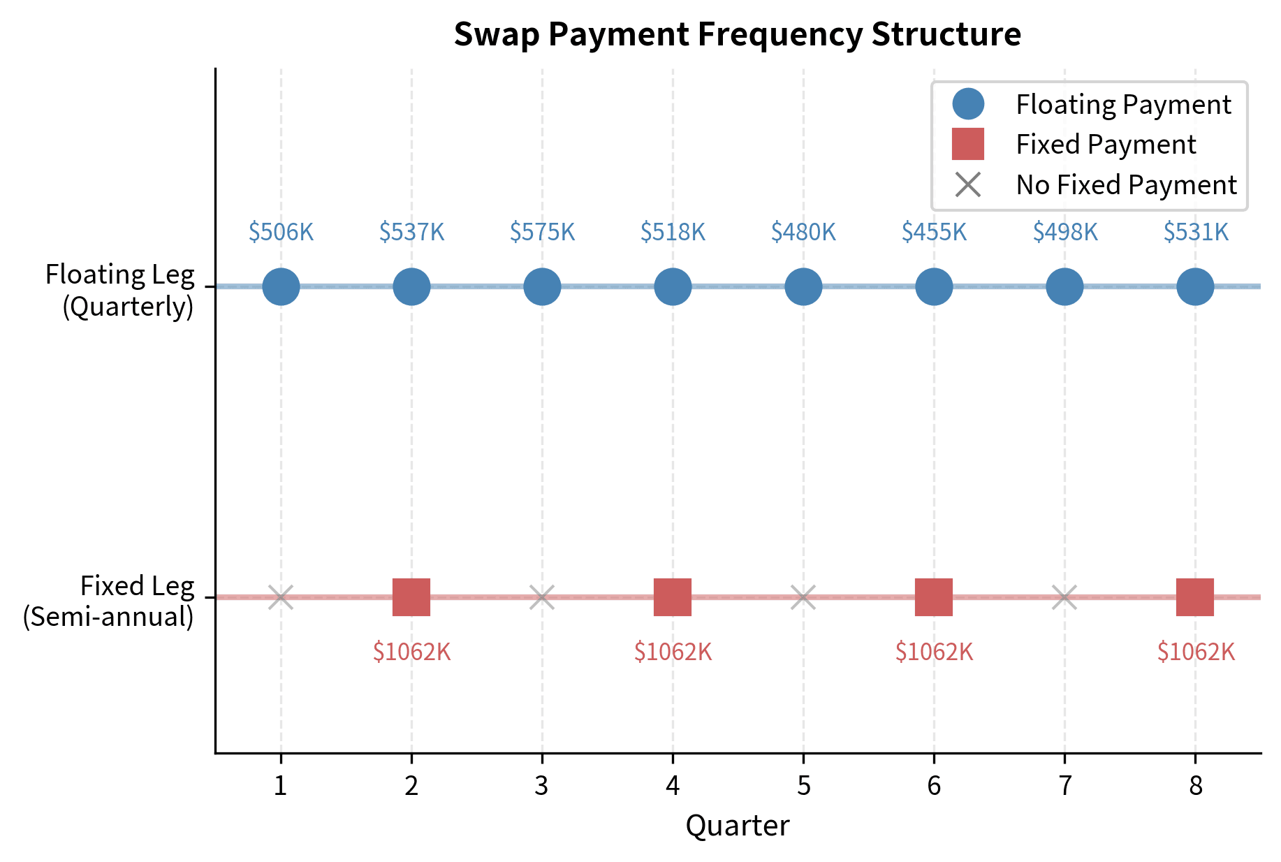
The structure of this swap means that fixed payments occur every six months (four total over two years), while floating payments occur every three months (eight total). This mismatch in payment frequencies is common and creates quarters where only the floating leg pays and quarters where both legs pay. Understanding this rhythm is essential for cash flow forecasting and liquidity planning.
Let's calculate the cash flows assuming we observe the following floating rates at each reset date:
This cash flow schedule illustrates several important features of swap mechanics. The fixed payments are predictable and occur semi-annually, while floating payments vary each quarter based on the prevailing reference rate. The net cash flow can be positive or negative in any period depending on whether floating rates are above or below the fixed rate. Notice also how the day count differences affect the calculations: the floating leg uses actual days (91 or 92), while the fixed leg calculation implicitly assumes 180 days per semi-annual period under the 30/360 convention.
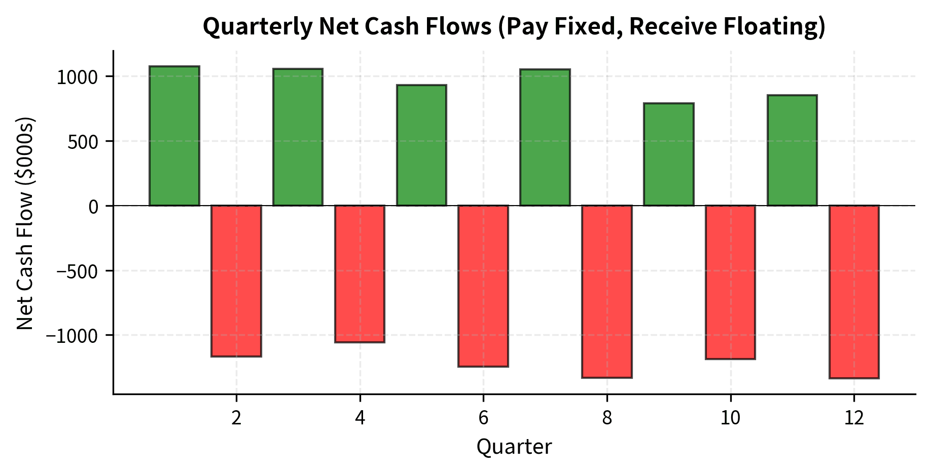
Visualizing Swap Cash Flows
A visual representation helps clarify the cash flow exchange structure. The bar chart format allows us to see both the individual payment components and the cumulative effect over time, providing insight into how the swap's profitability evolves as rates change.
The chart shows that the party paying fixed and receiving floating benefits when floating rates exceed the fixed rate. The cumulative net position tracks the overall profitability of the swap position over time.
Why Use Interest Rate Swaps?
Swaps serve multiple purposes in financial markets, ranging from hedging to speculation to balance sheet management. Understanding these motivations helps explain why the swap market grew so large.
Hedging Interest Rate Risk
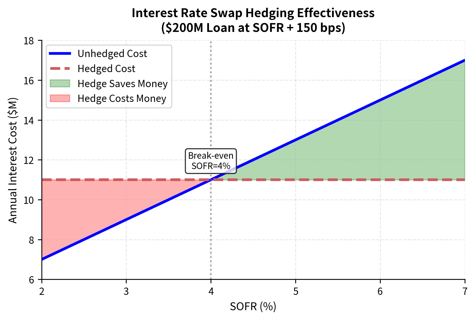
Consider a company that has issued floating-rate debt and wants to lock in its borrowing costs. Perhaps the company has \$200 million in bank loans tied to SOFR plus a credit spread. If interest rates rise, the company's interest expense increases, potentially straining cash flow.
By entering a pay-fixed, receive-floating swap with a notional of $200 million, the company effectively converts its floating-rate exposure to fixed. The floating payments received from the swap offset the floating payments on the loan, leaving only the fixed swap rate as the effective borrowing cost.
The analysis demonstrates the hedging power of swaps. Regardless of where SOFR moves, the hedged cost remains constant at the swap fixed rate plus the loan spread. When rates rise above expectations, the company saves money compared to the unhedged position. When rates fall, the company forgoes potential savings but has certainty about its costs.
Asset-Liability Management
Banks face a structural challenge: their deposits (liabilities) typically have short maturities and floating rates, while their loans (assets) often have longer maturities and fixed rates. This creates interest rate risk. If short-term rates rise, the bank's funding costs increase while its loan income stays fixed.
Swaps allow banks to manage this mismatch. A bank can enter pay-floating, receive-fixed swaps to better match its asset and liability characteristics. The fixed swap payments received help offset the fixed income from loans, while the floating payments made are funded by floating-rate deposits.
Comparative Advantage and Cost Reduction
The theoretical foundation for swaps rests partly on the principle of comparative advantage, familiar from international trade theory. Different borrowers face different credit spreads in fixed versus floating markets. A borrower may have an absolute advantage in one market (lower rates than competitors) but a comparative advantage in another (a relatively smaller disadvantage). When parties exploit these comparative advantages through swaps, both can benefit.
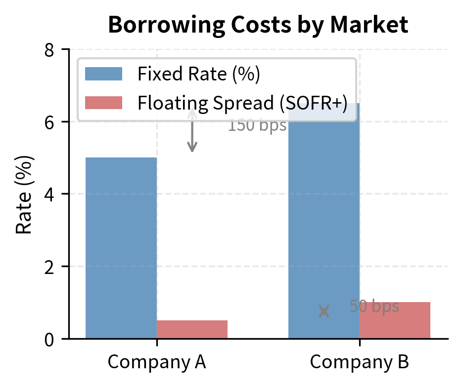
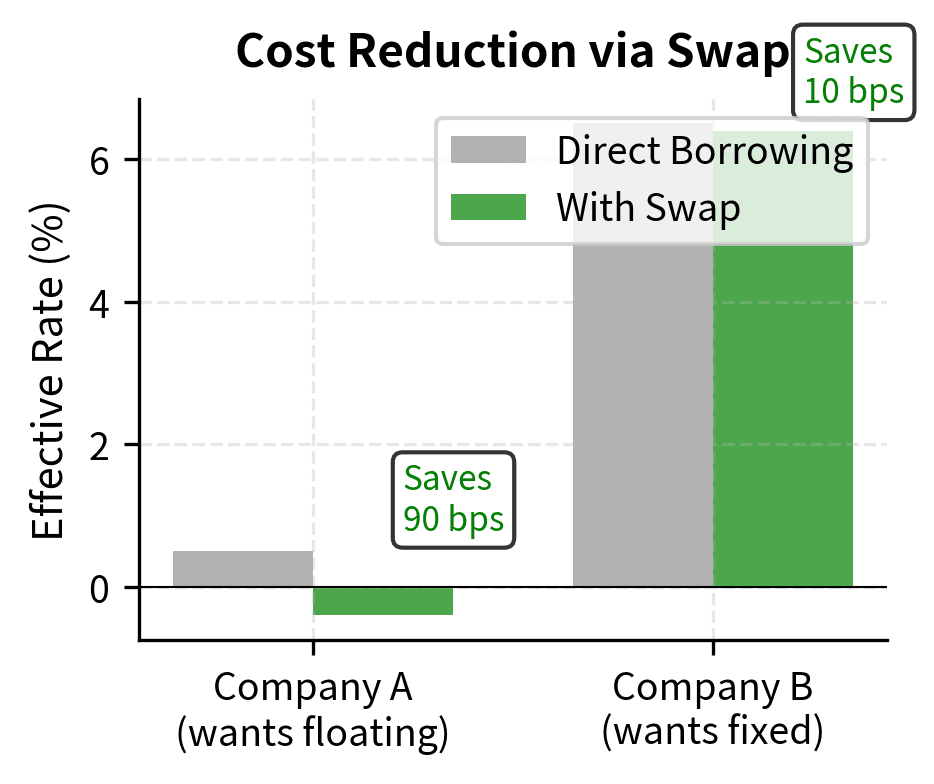
Suppose Company A can borrow at 5.0% fixed or SOFR + 0.5%, while Company B can borrow at 6.5% fixed or SOFR + 1.0%. Company A has an absolute advantage in both markets (lower rates in each), but the advantage is larger in the fixed market (150 basis points) than in the floating market (50 basis points). This difference in relative advantages creates an opportunity for mutually beneficial exchange.
This example shows how swaps can create value. Company A has a comparative advantage in fixed-rate markets, while Company B's disadvantage is smaller in floating markets. By borrowing in their respective advantage markets and swapping, both companies end up with lower costs than if they had borrowed directly in their desired market.
Speculation on Interest Rates
Traders and investors also use swaps to express views on interest rate movements. A trader expecting rates to rise might enter a receive-fixed, pay-floating swap. If rates indeed rise, the floating payments they make increase, but the swap's market value also increases (since the fixed rate they receive becomes more valuable relative to new market rates).
Unlike buying or selling bonds, swaps require no upfront capital beyond margin requirements. This leverage makes them efficient instruments for taking directional positions on rates.
Other Common Swap Types
While plain-vanilla interest rate swaps dominate the market, several other swap structures serve specialized needs.
Currency Swaps
Currency swaps extend the swap concept to exchange cash flows in different currencies. Unlike interest rate swaps where notional principal is never exchanged, currency swaps typically involve exchanging principal at both the start and end of the contract.
A currency swap is an agreement to exchange principal and interest payments in one currency for principal and interest payments in another currency. The exchange rates for these transactions are fixed at the contract's inception.
Consider a U.S. company that needs euros for a European subsidiary. Rather than borrowing directly in euros (where it may have limited access or higher costs), the company can borrow in dollars and enter a currency swap. At inception, it pays dollars and receives euros. Throughout the life of the swap, it pays euro interest and receives dollar interest. At maturity, the principal amounts are re-exchanged at the original exchange rate.
Currency swaps serve several purposes:
- Funding foreign operations: Companies can access foreign currency funding indirectly.
- Hedging foreign currency debt: A company with euro-denominated debt can hedge its exposure back to dollars.
- Exploiting funding advantages: Like interest rate swaps, currency swaps can exploit comparative advantages across different currency markets.
Commodity Swaps
Commodity swaps allow parties to exchange fixed payments for floating payments tied to commodity prices. An airline might enter a swap where it pays a fixed price per barrel of jet fuel and receives floating payments based on the actual market price. This hedges the airline's fuel cost exposure by converting uncertain future costs into known, budgetable amounts.
The structure mirrors interest rate swaps, with the commodity price replacing the interest rate in the calculation. The net payment for each settlement period is determined by comparing the agreed fixed price to the observed market price:
where:
- Notional Quantity: the volume of the commodity (e.g., barrels of oil)
- Fixed Price: the price per unit agreed upon at contract inception
- Floating Price: the market price per unit observed at the reset date
The formula shows that when the floating market price exceeds the fixed price, the net payment is negative for the fixed-price payer, meaning they receive a payment that offsets their higher actual purchasing costs. Conversely, when market prices fall below the fixed price, the fixed-price payer makes a net payment but benefits from lower actual purchase costs. The swap effectively locks in the fixed price regardless of market movements.
For a commodity consumer (like an airline), paying fixed and receiving floating locks in costs. For a producer (like an oil company), the opposite position locks in revenues.
Basis Swaps
A basis swap exchanges two different floating rates rather than fixed for floating. For example, a swap might exchange 3-month SOFR for 1-month SOFR plus a spread, or SOFR for another floating rate like the Fed Funds rate. These swaps are useful when a party has assets tied to one rate and liabilities tied to another.
Other Variations
The swap market's flexibility has led to numerous other structures:
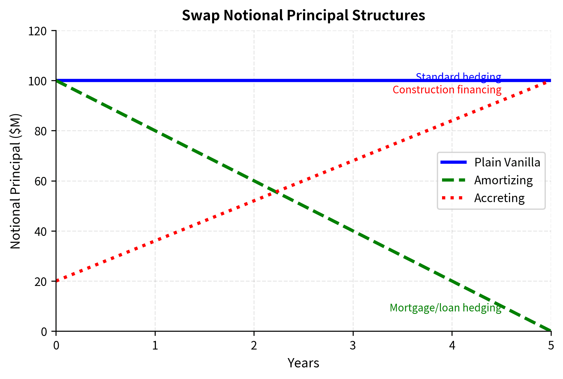
- Amortizing swaps: The notional principal decreases over time, matching amortizing loans.
- Accreting swaps: The notional principal increases over time, useful for construction financing.
- Forward-starting swaps: The swap becomes effective at a future date, allowing parties to lock in rates ahead of anticipated funding needs.
- Overnight index swaps (OIS): Exchange a fixed rate for a compounded overnight rate, used extensively for managing short-term funding and as a benchmark for risk-free rates.
Market Structure and Conventions
Understanding how the swap market operates helps explain both its utility and its risks.
Over-the-Counter Nature
Swaps trade in the OTC market, meaning they are negotiated directly between counterparties rather than through a central exchange. Historically, this meant each swap was a bespoke contract between two parties, with terms tailored to their specific needs.
The OTC structure provides flexibility but creates challenges:
- Counterparty credit risk: Each party bears the risk that the other may default on their obligations.
- Lack of transparency: Without a central exchange, price discovery was historically less efficient.
- Operational complexity: Managing thousands of bilateral contracts requires sophisticated systems.
Post-Crisis Reforms
The 2008 financial crisis exposed vulnerabilities in the OTC derivatives market. The failure of Lehman Brothers left its swap counterparties with massive losses and uncertainty about their positions. In response, regulators mandated significant reforms.
The Dodd-Frank Act in the United States and similar regulations globally required:
- Central clearing: Standardized swaps must be cleared through central counterparties (CCPs), which guarantee performance and reduce counterparty risk.
- Trade reporting: All swap transactions must be reported to trade repositories, improving transparency.
- Margin requirements: Both cleared and uncleared swaps require initial and variation margin, reducing credit exposure.
- Trading on regulated platforms: Certain standardized swaps must be traded on swap execution facilities (SEFs) rather than purely bilaterally.
These reforms have substantially changed the swap market, reducing systemic risk while increasing costs and standardization.
Swap Conventions
Standard swap conventions vary by currency and have evolved over time. For U.S. dollar interest rate swaps, typical conventions include:
ISDA Documentation
The International Swaps and Derivatives Association (ISDA) has developed standardized documentation that governs most swap transactions. The ISDA Master Agreement provides a framework for all transactions between two parties, covering events of default, termination, and netting. Individual transactions are documented in trade confirmations that reference the Master Agreement.
This standardization, while adding some rigidity, dramatically reduced legal uncertainty and operational complexity in the swap market.
Building a Swap Cash Flow Calculator
Let's build a more complete implementation that can generate swap cash flow schedules for analysis. This calculator demonstrates how the concepts we have discussed translate into practical computation. The function takes swap parameters as inputs and produces a detailed schedule showing each payment throughout the swap's life.
Now let's use this function to analyze a swap:
Visualizing the Swap Profile
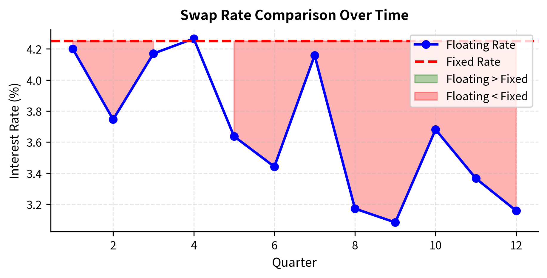
The visualization shows the relationship between the fixed and floating rates and the resulting net cash flows. Green regions indicate periods where floating rates exceed the fixed rate, generating positive net cash flows for the fixed-rate payer. Red regions show the opposite situation.
Limitations and Practical Considerations
While swaps are powerful risk management tools, they come with important limitations and risks that you must understand.
Counterparty Credit Risk
The most significant risk in swap transactions is counterparty credit risk: the possibility that the other party will default on their obligations. This risk is asymmetric, since only the party with a positive market value on the swap (the "in-the-money" party) faces exposure. A swap can be an asset to one party and a liability to the other, and these positions can flip as interest rates move.
Central clearing has substantially mitigated this risk for standardized swaps. When a swap is cleared, the central counterparty (CCP) becomes the counterparty to both original parties, guaranteeing performance. The CCP manages risk through initial margin requirements, daily variation margin calls, and default funds contributed by clearing members. However, uncleared swaps, particularly customized contracts, still carry bilateral counterparty risk.
Basis Risk
When using swaps to hedge, the hedge may not perfectly match the underlying exposure. This basis risk can arise from several sources. The floating rate on the swap might not exactly match the floating rate on the hedged liability. A company hedging SOFR-based loans with a swap might find that its loan resets on different dates than the swap, or uses different calculation methods. Additionally, the notional amount of the hedge might not perfectly match the exposure, or the hedge might have different payment dates than the underlying.
Liquidity Risk
While the swap market is generally liquid for standard tenors (1, 2, 3, 5, 7, 10, and 30 years) in major currencies, liquidity can deteriorate during market stress. In 2008 and again in March 2020, bid-ask spreads widened dramatically, and some counterparties pulled back from market-making. This can make it difficult to exit or adjust positions precisely when hedging is most needed.
Regulatory and Documentation Complexity
The post-crisis regulatory environment has added significant complexity to swap transactions. Reporting requirements, margin rules, and clearing mandates require sophisticated operational infrastructure. The ISDA documentation framework, while standardized, is lengthy and requires legal expertise to navigate. For smaller market participants, these costs can make swaps less accessible.
The LIBOR Transition Impact
The transition from LIBOR to SOFR created substantial operational challenges. Legacy contracts referencing LIBOR had to be amended, and the economic impact of the spread adjustment between LIBOR and SOFR was significant for some portfolios. While the transition is largely complete, it serves as a reminder that "permanent" market conventions can change, requiring flexibility in systems and documentation.
Summary
Interest rate swaps have transformed how corporations, banks, and investors manage interest rate risk. By allowing parties to exchange fixed and floating cash flows without exchanging principal, swaps provide a flexible and capital-efficient mechanism for hedging and speculation.
The key concepts from this chapter include:
- Swap structure: Plain-vanilla swaps exchange fixed interest payments for floating payments based on a reference rate, with the notional principal serving only as a calculation base.
- Cash flow mechanics: Fixed leg payments use conventions like 30/360 day count, while floating legs typically use Actual/360. Payments are usually netted, with only the difference exchanged.
- Reference rates: The transition from LIBOR to SOFR represents a fundamental shift in how floating rates are determined, moving from estimated rates to transaction-based rates.
- Applications: Swaps serve multiple purposes including hedging interest rate exposure, managing asset-liability mismatches, exploiting comparative advantages in credit markets, and expressing views on rate movements.
- Other swap types: Currency swaps exchange cash flows in different currencies, commodity swaps hedge price exposure, and basis swaps exchange different floating rates.
- Market structure: Post-crisis reforms have pushed standardized swaps toward central clearing and transparent trading, while customized contracts remain bilateral.
In the next chapter, we'll explore swap valuation and more advanced applications, building on the cash flow foundations established here. Understanding how to price swaps at inception and mark them to market throughout their lives is essential for both trading and risk management.
Quiz
Ready to test your understanding? Take this quick quiz to reinforce what you've learned about interest rate swaps.

Comments