

Learn the Black-Scholes formula for European options with Python implementation. Covers derivation, the Greeks, put-call parity, and dividend adjustments.
Choose your expertise level to adjust how many terms are explained. Beginners see more tooltips, experts see fewer to maintain reading flow. Hover over underlined terms for instant definitions.
Black-Scholes Formula and European Option Pricing
In the previous chapter, we derived the Black-Scholes-Merton partial differential equation (PDE), which describes how the price of a derivative must evolve to prevent arbitrage opportunities. That PDE, while elegant, doesn't immediately tell us what an option is worth. To actually price an option, we need to solve the PDE subject to the appropriate boundary conditions.
This chapter presents the solution: the famous Black-Scholes formula for European options. Published by Fischer Black and Myron Scholes in 1973, with crucial contributions from Robert Merton, this formula transformed finance by providing the first closed-form solution for option prices. Before Black-Scholes, options traded with wide bid-ask spreads because traders couldn't agree on fair value. After Black-Scholes, the options market exploded in both volume and sophistication.
The formula expresses an option's price in terms of five observable or estimable quantities: the current stock price, the strike price, time to expiration, the risk-free interest rate, and the volatility of the underlying asset. The expected return of the stock does not appear in the formula. As we learned when studying risk-neutral valuation, we can price derivatives by pretending all assets grow at the risk-free rate, a consequence of the no-arbitrage principle.
We'll work through the solution to the Black-Scholes PDE, interpret each component of the resulting formula, implement it in Python, and verify that it satisfies fundamental relationships like put-call parity. We'll close with an introduction to the Greeks, the sensitivity measures that quantify how option prices respond to changes in the underlying parameters.
Solving the Black-Scholes PDE
Recall from the previous chapter that the Black-Scholes PDE for a derivative on a non-dividend-paying stock is:
where:
- : price of the derivative
- : time
- : price of the underlying asset
- : volatility of the underlying asset
- : risk-free interest rate
This equation captures a fundamental requirement: the price of any derivative must evolve in time so no riskless arbitrage profit can be extracted. Each term in the equation plays a specific role. The first term represents how the option price changes with the passage of time alone. The second term, involving the second derivative with respect to the stock price, captures the effect of the stock's random fluctuations, which is precisely why the volatility parameter appears squared and multiplied by . The third term accounts for the drift in the option price due to the expected growth of the stock under risk-neutral dynamics. Finally, the last term ensures that the total return on any derivative equals the risk-free rate in a hedged portfolio.
To find the price of a European call option, we must solve this PDE subject to the boundary condition at expiration:
where:
- : value of the call option at expiration
- : stock price at expiration
- : strike price
- : expiration time
This boundary condition states something intuitive: at the moment of expiration, an option is worth exactly its intrinsic value. If the stock price exceeds the strike, the call holder can buy the stock at and immediately sell it at , pocketing the difference. If the stock price falls below the strike, the call expires worthless. The mathematical challenge lies in determining what the option should be worth at any time before expiration, given that it will satisfy this terminal condition.
Transformation to the Heat Equation
The Black-Scholes PDE is a second-order linear parabolic PDE. While it looks complicated, it can be transformed into the heat equation, one of the most studied equations in mathematical physics. This transformation involves several changes of variables. Instead of solving the Black-Scholes PDE directly, we convert it into the well-studied heat equation. The heat equation describes how temperature diffuses through a material, and its solutions are extremely well understood.
First, we introduce dimensionless variables. Let represent time to expiration, so increases as we move backward from expiration. This reversal of time direction is natural because we know the option's value at expiration and want to work backward to find its present value. Define to work with log-prices. This logarithmic transformation converts the multiplicative nature of stock price movements into an additive one, which simplifies the mathematics considerably. A stock that can move between $50 and $200 has log-price that ranges from to , a much more symmetric range to work with. Finally, let be a transformed version of the option price:
where:
- : original option price
- : strike price
- : risk-free rate
- : time to expiration
- : transformed option price
- : log-price variable
The factor accounts for the time value of money, essentially expressing the transformed price in forward terms. The factor scales the problem so that the transformed variable is dimensionless, depending only on relative moneyness rather than absolute dollar amounts.
Applying these substitutions and simplifying using the chain rule transforms the Black-Scholes PDE into:
where:
- : transformed option price
- : time to expiration
- : log-price variable
- : volatility
- : risk-free rate
This equation is already simpler than the original because the coefficients are now constants rather than functions of . However, it still contains a first derivative term, which represents a drift in the log-price. To eliminate this drift and arrive at the standard heat equation, we perform one more transformation.
A further substitution of the form eliminates the first derivative term. By choosing the constants and appropriately, specifically values that depend on the ratio of the risk-free rate to the volatility squared, we can make the first-order term vanish. This yields the standard heat equation:
where:
- : variable related to option price (after removing drift)
- : time to expiration
- : spatial variable (log-price)
- : volatility parameter
The heat equation has a well-known solution via the Green's function, also called the fundamental solution or heat kernel. The physical interpretation is illuminating: if you place a concentrated source of heat at a single point and watch how it spreads through a material, the temperature at any point and time is given by a Gaussian distribution centered at the original source. The solution involves convolving the initial condition with this Gaussian kernel, essentially averaging over all possible paths the "heat" (or in our case, the probability mass) could have traveled.
The General Solution
Working backward through the transformations, reversing each change of variables in sequence, the solution for a European call option emerges as:
where:
- : call option price
- : current stock price
- : cumulative standard normal distribution function
- : standardized moneyness terms
- : strike price
- : risk-free interest rate
- : time to expiration
This formula expresses the option price as the difference between two terms, each involving the cumulative normal distribution function . The function gives the probability that a standard normal random variable is less than , and it appears here because the underlying stock price follows a lognormal distribution under geometric Brownian motion.
The terms and are defined as:
where:
- : current stock price
- : strike price
- : risk-free rate
- : volatility
- : time to expiration
The numerator of contains two parts. The first, , measures the current moneyness of the option in logarithmic terms. A positive value indicates the option is in-the-money, while a negative value indicates it is out-of-the-money. The second part, , represents the expected drift of the log-price over the remaining life of the option. The denominator, , normalizes this quantity by the standard deviation of the log-price at expiration, converting it into a standardized z-score.
The second standardized term is:
where:
- : first standardized term
- : volatility
- : time to expiration
- : current stock price
- : strike price
- : risk-free rate
Notice that differs from only in the sign of the term in the numerator. This seemingly small difference has a profound interpretation that we will explore shortly. The relationship shows that the two quantities differ by exactly one standard deviation of the log-return.
For a European put option, we can either solve the PDE with the put boundary condition , or use put-call parity. The result is:
where:
- : put option price
- : strike price
- : risk-free rate
- : time to expiration
- : current stock price
- : cumulative standard normal distribution function
- : standardized moneyness terms
The put formula has a parallel structure to the call formula but with the terms reversed and the signs of the arguments to flipped. This symmetry reflects the complementary nature of calls and puts: a call benefits when the stock rises above the strike, while a put benefits when the stock falls below the strike. The relationship between the two formulas is made precise by put-call parity.
These are the celebrated Black-Scholes formulas. Let's examine what each term means.
Anatomy of the Black-Scholes Formula
The call option formula (where ) has a clear interpretation when viewed through the lens of risk-neutral valuation. To understand the formula, we must connect it to risk-neutral pricing, where a derivative's price is its discounted expected payoff:
where:
- : call option price
- : risk-free rate
- : time to expiration
- : expectation under the risk-neutral measure
- : stock price at expiration
- : strike price
This expectation says that we imagine a world where all investors are indifferent to risk, so the stock grows at the risk-free rate on average. In this risk-neutral world, we calculate the average payoff of the option and then discount it back to today. This procedure gives the correct arbitrage-free price even though the real world is not risk-neutral.
This expectation can be decomposed into two pieces:
where:
- : call option price
- : risk-free rate
- : time to expiration
- : stock price at expiration
- : strike price
- : indicator function (1 if , 0 otherwise)
- : probability under the risk-neutral measure
This decomposition separates the option's payoff into its two components: receiving the stock and paying the strike. The indicator function equals 1 when the option finishes in-the-money and 0 otherwise. The first term captures the expected value of receiving the stock in those scenarios where exercise occurs. The second term captures the expected cost of paying the strike price, again only in scenarios where exercise occurs.
The second term is straightforward: is the present value of paying the strike, weighted by the risk-neutral probability that the option finishes in-the-money. This term has a clean economic interpretation. You can think of it as the cost of a contingent payment: you will pay at expiration, but only if . The probability of this event under risk-neutral dynamics is , and we discount the expected payment back to today at the risk-free rate.
The first term requires more care. represents the present value of receiving the stock conditional on exercise. The factor isn't quite a probability in the usual sense. It is the expected stock price conditional on exercise, normalized appropriately. To be precise, when you compute the expected value of the stock price over only those outcomes where , you get a number that depends not just on the probability of exercise but also on how high the stock price tends to be in those favorable scenarios. Stocks that are likely to exercise tend to be worth more when they do exercise, which creates a positive correlation that inflates the expected receipt above what simple probability would suggest.
Technically, is the probability that under a different probability measure, sometimes called the stock measure or share measure. This alternative measure reweights outcomes according to the stock price, giving more weight to high-stock-price scenarios. Under this measure, the probability of exercise is higher than because we are overweighting exactly those outcomes where exercise occurs. The difference between and captures this reweighting effect.
The Role of Each Parameter
The five inputs to the Black-Scholes formula each affect option prices in intuitive ways. Understanding these relationships builds intuition for how options behave and why traders care about each parameter.
-
Stock price (): Higher stock prices increase call values and decrease put values. This is the most direct relationship: a call gives you the right to buy at , so the higher is relative to , the more valuable that right. If the stock is already trading at $120 and your strike is $100, the option has $20 of intrinsic value plus whatever time value remains. Mathematically, the stock price enters the formula directly in the first term and indirectly through and .
-
Strike price (): Higher strikes decrease call values and increase put values. A call with a higher strike requires the stock to rise further to be profitable. Consider two calls, one with strike $100 and another with strike $110. The first call is easier to profit from because the stock needs only to exceed $100, not $110. The strike enters the formula in the second term and in the logarithm within and .
-
Time to expiration (): More time generally increases option values. This "time value" reflects the increased opportunity for favorable price movements. A six-month option has more time for the stock to make a large move than a one-month option. The relationship enters through in the formula, meaning time value doesn't grow linearly. This square root dependence is crucial: the first month of a six-month option is less valuable than the first month of a one-month option. Options lose value at an accelerating rate as expiration approaches, a phenomenon called time decay.
-
Risk-free rate (): Higher rates increase call values and decrease put values. The intuition is that buying a call is like a leveraged position in the stock. You get stock exposure while keeping your capital earning interest elsewhere. Higher rates make this implicit financing benefit more valuable. Additionally, higher rates reduce the present value of the strike payment, making it cheaper in today's dollars to acquire the stock at expiration.
-
Volatility (): Higher volatility increases both call and put values. This is perhaps the most important insight of the model. Because an option's downside is limited (you can only lose the premium), higher volatility creates more upside potential without proportionally increasing downside risk. Consider a call option when the stock is at $100 and the strike is $100. If volatility is very low, the stock will likely stay near $100 and the option will be worth little. If volatility is high, the stock might reach $120 or $80 with meaningful probability. The $120 outcome pays $20, while the $80 outcome pays nothing. Higher volatility increases the chance of reaching $120 without increasing the cost of the $80 outcome which is already zero.
Four of the five Black-Scholes inputs are directly observable: you can look up the stock price, strike price, time to expiration, and risk-free rate. Only volatility must be estimated. This makes volatility the central challenge in option pricing, a topic we'll explore in depth when we study implied volatility and the volatility smile.
Understanding and
The quantities and are standardized measures of "moneyness," expressing how far in- or out-of-the-money the option is, adjusted for time and volatility. These quantities serve as the arguments to the cumulative normal distribution function, converting the lognormal distribution of stock prices into a tractable form.
Consider first:
where:
- : stock price
- : strike price
- : risk-free rate
- : volatility
- : time to expiration
To understand , we need to recall how the stock price evolves under geometric Brownian motion. The numerator is the expected log-return of the stock under the risk-neutral measure, relative to the strike. The term appears rather than just because of the difference between arithmetic and geometric means. When a variable follows geometric Brownian motion with drift , its expected logarithm grows at rate , not . This correction factor, sometimes called the Itô correction or convexity adjustment, arises from the nonlinear relationship between a variable and its logarithm.
Recall that under geometric Brownian motion with drift , the expected log-price is:
where:
- : expected log stock price at time
- : log of current stock price
- : risk-free rate
- : volatility
- : time to expiration
So the numerator equals . This is the expected value of the log of the ratio of the terminal stock price to the strike. When this is positive, the stock is expected to end up above the strike on average. The denominator is the standard deviation of this log-return. The volatility of the log-price after time is , reflecting the diffusion of prices over time. Thus measures how many standard deviations the expected log-price exceeds the log-strike, which is exactly the input you'd need to find using the normal distribution.
The quantity is similar but with a term instead of . This difference of accounts for the convexity adjustment when computing expected values of lognormal variables. When we compute not just the probability of exercise but the expected stock price conditional on exercise, we need to account for the asymmetry of the lognormal distribution. High stock prices are further above the mean than low stock prices are below it, and this asymmetry inflates the expected value conditional on exceeding a threshold.
The technical explanation involves a change of measure: is a probability under a different measure where the stock, rather than the money market account, is the numeraire. In this alternative measure, the stock price process has a higher drift, compensating for the fact that we're measuring things in stock units rather than dollar units. The result is that probabilities under the stock measure are systematically higher than under the risk-neutral measure for in-the-money events.
Put-Call Parity Revisited
As we learned when studying option basics, put-call parity is a fundamental relationship linking European call and put prices:
where:
- : call option price
- : put option price
- : stock price
- : strike price
- : risk-free rate
- : time to expiration
This relationship must hold regardless of any model assumptions; it is a pure arbitrage argument. If it were violated, you could construct a riskless profit by simultaneously buying the cheap side and selling the expensive side. The relationship says that a portfolio of a long call and a short put with the same strike and expiration replicates the payoff of owning the stock while owing the present value of the strike price.
Let's verify that the Black-Scholes formulas satisfy put-call parity. This verification serves two purposes: it confirms that our formulas are internally consistent, and it demonstrates the elegant symmetry properties of the normal distribution.
Starting with the Black-Scholes call and put formulas:
where:
- : call and put option prices
- : stock price
- : strike price
- : risk-free rate
- : time to expiration
- : cumulative standard normal distribution
- : moneyness terms
We compute the difference to verify the relationship. The key mathematical fact we will use is the symmetry of the standard normal distribution: for any value of . This follows from the fact that the normal distribution is symmetric around zero, so the probability of being less than plus the probability of being greater than (which equals the probability of being less than ) must sum to one.
where:
- : call price
- : put price
- : stock price
- : strike price
- : risk-free rate
- : time to expiration
The Black-Scholes formulas are internally consistent and satisfy the no-arbitrage constraint of put-call parity. This verification is more than a mathematical exercise. It confirms that the formulas respect the fundamental arbitrage relationships that must hold in any well-functioning market. Any pricing model, no matter how sophisticated, must satisfy put-call parity. If a proposed option pricing formula violated this relationship, we would know immediately that it contains an error.
Implementing the Black-Scholes Formula
Let's implement the Black-Scholes formula in Python and explore its behavior. We'll build up from simple functions to a complete implementation.
Now let's calculate option prices for a specific example:
The call option on this slightly out-of-the-money stock has a lower value than the put, which holds intrinsic value. Let's verify put-call parity holds:
The difference of effectively zero confirms that our implementation satisfies the fundamental no-arbitrage relationship required by put-call parity.
Examining the Intermediate Calculations
Understanding the intermediate values and helps build intuition for how the formula works:
The negative value tells us there's less than a 50% risk-neutral probability that this option finishes in-the-money. The value of calculated above represents the precise probability of the stock price exceeding the strike at expiration under the risk-neutral measure.
Key Parameters
The key parameters for the Black-Scholes implementation are:
- : Current stock price. Higher prices increase call values and decrease put values.
- : Strike price. The reference price for the option's payoff.
- : Time to expiration in years. Longer times generally increase option values.
- : Risk-free interest rate (annualized). Higher rates favor calls over puts.
- : Volatility (annualized). Determines the range of potential future stock prices; higher volatility increases value for both calls and puts.
Option Price Sensitivity to Inputs
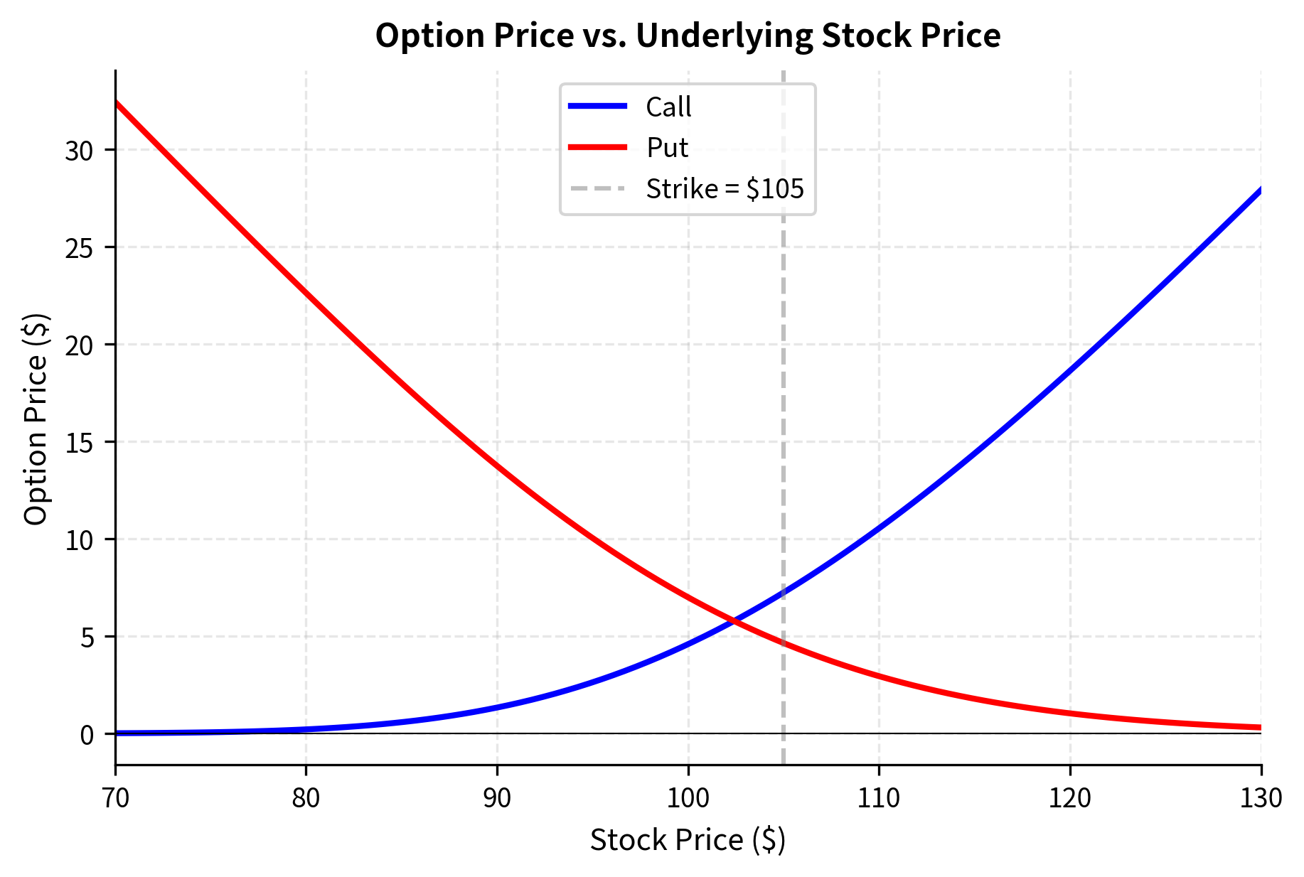
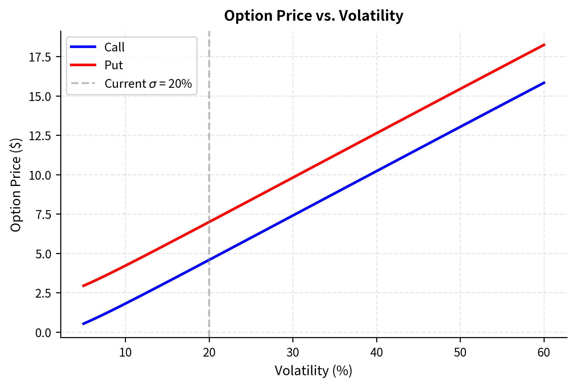
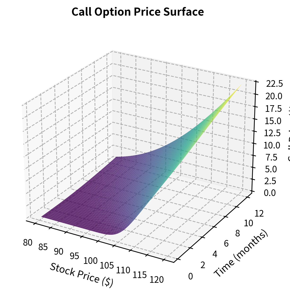
Let's visualize how option prices change with respect to each input parameter. This builds intuition for the Greeks, which we'll introduce formally later in this chapter.
The curves show the characteristic "hockey stick" shape approaching expiration, but smoothed by time value. Notice how both options have positive value even when out-of-the-money. This is the time value component.
The monotonic relationship between option prices and volatility is crucial. Since all other inputs are directly observable, if you know an option's market price, you can "invert" the Black-Scholes formula to find the volatility that would produce that price. This implied volatility becomes a key market observable, which we'll study in a later chapter.
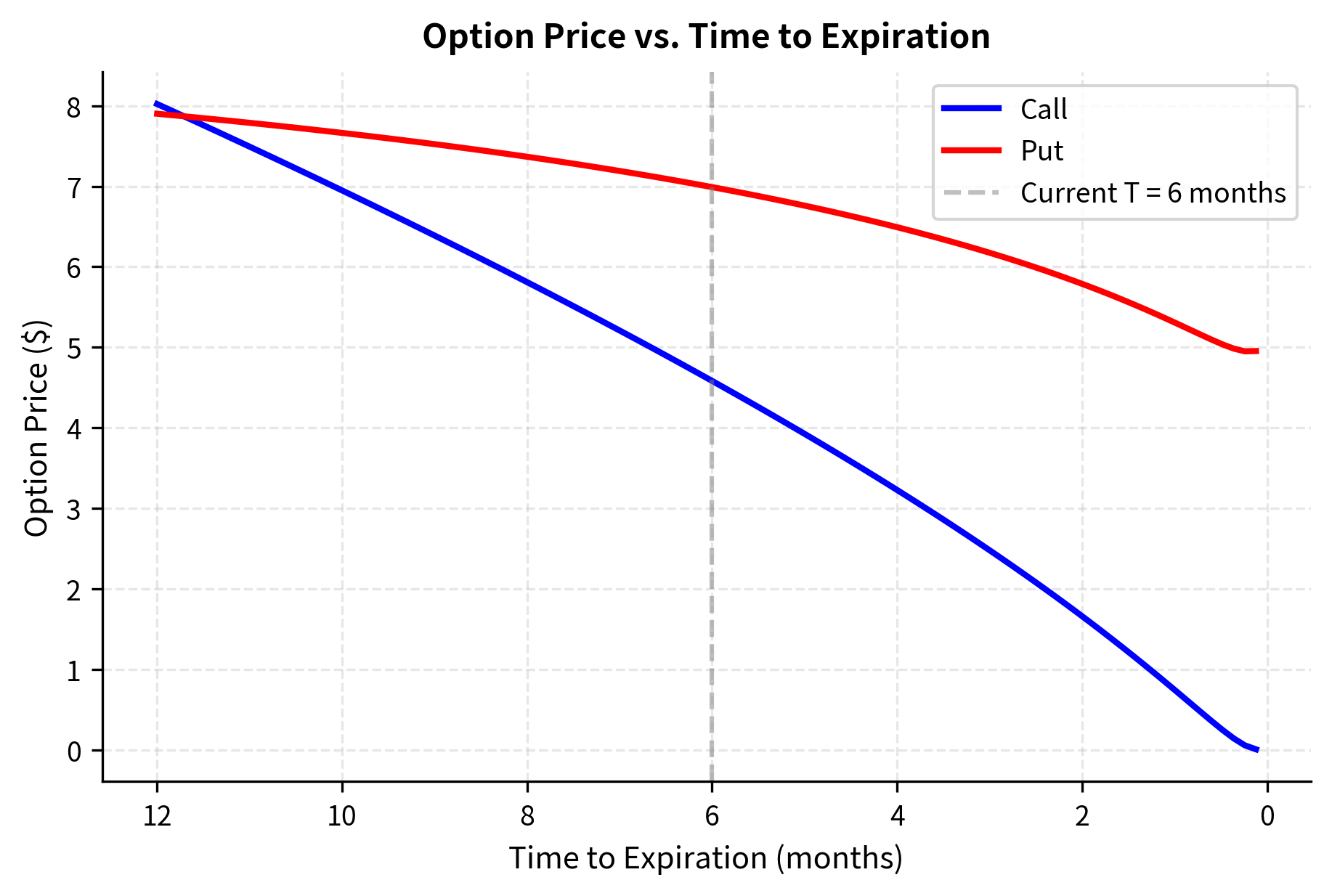
As time passes, option prices decay toward their intrinsic values. This time decay (quantified by the Greek letter theta) is a critical consideration for option traders, particularly those holding long positions.
Introduction to the Greeks
The Greeks are partial derivatives of the option price with respect to various inputs. They quantify how sensitive an option's price is to small changes in market conditions. Understanding the Greeks is essential for risk management and hedging. Each Greek measures a different dimension of risk, and together they provide a complete picture of an option position's exposure to market movements.
The Greeks derive their importance from the dynamic nature of hedging. As we learned when studying the derivation of the Black-Scholes PDE, perfect replication of an option requires continuous adjustment of a hedge portfolio. The Greeks tell us exactly how to perform these adjustments and quantify the risks that arise when hedging is imperfect or infrequent.
The Greeks are named after Greek letters and measure the sensitivity of option prices to changes in underlying parameters. The five primary Greeks are Delta, Gamma, Theta, Vega (not actually Greek), and Rho.
Delta: Sensitivity to Stock Price
Delta () measures how much the option price changes when the stock price moves by $1. This is the most fundamental Greek because it directly connects the option's value to movements in the underlying asset. Delta answers the practical question: if the stock moves, how much does your option position change in value?
where:
- : delta of the call option
- : call option price
- : stock price
- : cumulative normal distribution value at
The result that call delta equals comes directly from differentiating the Black-Scholes formula. The derivative of the first term with respect to is not simply because itself depends on . However, when we carefully apply the chain rule, the additional terms cancel out, leaving just . This cancellation is not coincidental; it reflects a deep property of the Black-Scholes formula related to the self-financing nature of the replicating portfolio.
where:
- : delta of the put option
- : put option price
- : stock price
- : cumulative normal distribution value at
- : cumulative normal distribution value at
Call deltas range from 0 to 1, while put deltas range from -1 to 0. An at-the-money call has a delta near 0.5, meaning it moves about $0.50 for every $1 move in the stock. A deep in-the-money call has delta close to 1, moving nearly dollar-for-dollar with the stock. A deep out-of-the-money call has delta close to 0, barely responding to stock movements because the option is unlikely to ever be exercised.
Delta also has an interpretation as a hedge ratio: to hedge a short call position, you should hold shares of stock. If you sell a call with delta 0.5, you need to buy 0.5 shares to neutralize your exposure to small stock price movements. This hedge ratio must be continuously updated as the stock price moves and as time passes, which is why delta hedging is dynamic rather than static.
Gamma: Sensitivity of Delta to Stock Price
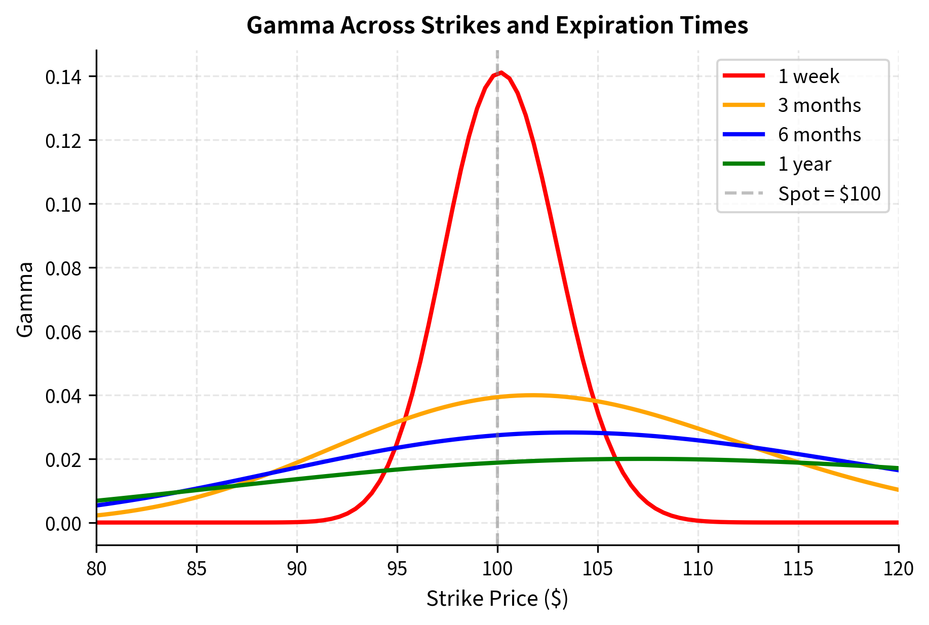
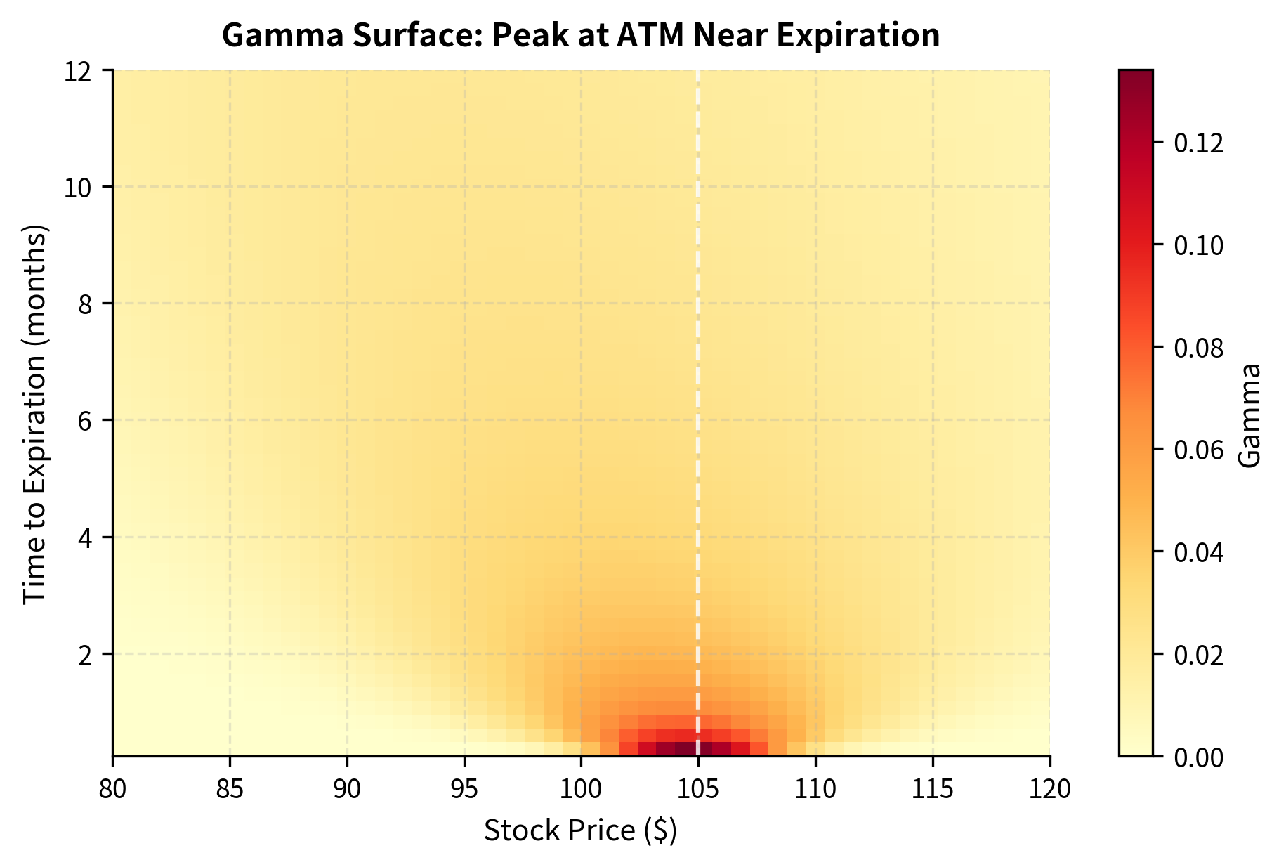
Gamma () measures how quickly delta changes as the stock moves by $1. This second-order sensitivity is crucial because it tells us how stable our delta hedge will be. High gamma means that even small moves in the stock price will significantly change the delta, requiring frequent rebalancing of the hedge.
where:
- : gamma of the option
- : option price (call or put)
- : stock price
- : standard normal probability density at
- : volatility
- : time to expiration
Note that is the standard normal probability density function. The appearance of the PDF rather than the CDF in gamma reflects the fact that gamma measures the rate of change of a probability. When the stock price moves, the probability of exercise changes, and gamma quantifies how rapidly this change occurs.
Gamma is the same for calls and puts with the same strike and expiration. This equality follows from put-call parity: since , and the right-hand side is linear in , the second derivative with respect to must be identical for calls and puts.
High gamma means the option's delta is unstable, requiring frequent rebalancing of hedges. At-the-money options near expiration have the highest gamma because small price movements can flip the option from out-of-the-money to in-the-money or vice versa, causing dramatic changes in delta. Gamma is a double-edged sword: long gamma positions benefit from realized volatility through the convexity of their payoff, but they also face the cost and complexity of frequent rebalancing.
Theta: Sensitivity to Time
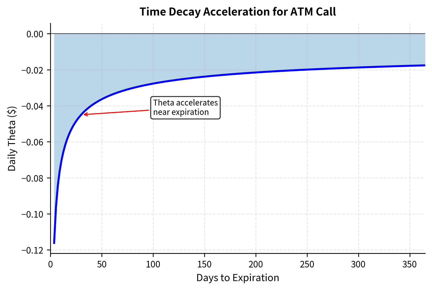
Theta () measures how much the option price decreases as time passes, holding all else constant. This is the only Greek that does not measure sensitivity to a market variable; instead, it captures the inexorable erosion of time value as expiration approaches. Time is the one factor that moves in only one direction, making theta fundamentally different from other risks.
where:
- : theta of the call option
- : stock price
- : standard normal PDF at
- : volatility
- : time to expiration
- : risk-free rate
- : strike price
- : cumulative normal CDF at
The formula consists of two components, each with a distinct economic interpretation:
- : Represents the erosion of value due to the resolution of uncertainty (volatility decay). As time passes, there is less time for favorable price movements to occur. This term is always negative, reflecting the fact that options lose optionality value over time.
- : Represents the loss of the interest-free leverage benefit as expiration approaches. A call option allows you to defer payment of the strike price until expiration. As expiration nears, this deferral benefit shrinks. For puts, this term has the opposite sign because puts involve receiving the strike rather than paying it.
Theta is typically negative for long option positions. Options lose value as time passes. This is the "cost" of holding optionality. The magnitude of theta increases as expiration approaches, especially for at-the-money options. This acceleration of time decay near expiration is sometimes called "time decay speeding up" and is a critical concern for option holders.
The relationship between theta and gamma is fundamental. The Black-Scholes PDE can be rearranged to show that, for a delta-hedged position, theta plus a term proportional to gamma must sum to the risk-free rate times the option value. This theta-gamma tradeoff means that positions with high positive gamma (which benefit from volatility) must pay high negative theta (losing value over time), and vice versa.
Vega: Sensitivity to Volatility
Vega ( or ) measures how much the option price changes when volatility moves by one percentage point. Despite being called "vega," this Greek is not named after an actual Greek letter, but the convention is so established that the name persists. Vega is arguably the most important Greek for option traders because volatility is the only unobservable input to the Black-Scholes formula and the one where traders have the most disagreement.
where:
- : vega of the option
- : option price
- : stock price
- : time to expiration
- : standard normal PDF at
Vega is the same for calls and puts and is always positive; higher volatility benefits option holders. This makes economic sense: volatility expands the range of possible future stock prices, and since options have limited downside (you can never lose more than the premium) but unlimited upside, more dispersion in outcomes is always favorable.
Vega is largest for at-the-money options and for options with longer time to expiration. At-the-money options are most sensitive to volatility because they are on the knife's edge between expiring worthless and expiring with value. Small changes in volatility significantly affect the probability of crossing the strike. Longer-dated options have more vega because there is more time for volatility to manifest as actual price movements.
When traders speak of "trading volatility," they typically mean taking positions that profit from changes in implied volatility. A trader who buys options has positive vega exposure and profits if volatility rises. A trader who sells options has negative vega exposure and profits if volatility falls.
Rho: Sensitivity to Interest Rate
Rho () measures how much the option price changes when the risk-free rate moves. Interest rate sensitivity is typically smaller than sensitivity to other parameters, but it can become significant for long-dated options or in environments where rates are changing rapidly.
where:
- : rho of the call option
- : strike price
- : time to expiration
- : risk-free rate
- : cumulative normal CDF at
Call rho is positive because higher interest rates reduce the present value of the strike payment while leaving the current stock price unchanged. A call holder benefits from this because they pay the strike in the future, and higher rates make that future payment cheaper in today's dollars.
where:
- : rho of the put option
- : put option price
- : strike price
- : time to expiration
- : risk-free rate
- : cumulative normal CDF at
Put rho is negative because put holders receive the strike price upon exercise. Higher interest rates make this future receipt less valuable in present terms. The magnitude of rho is proportional to time to expiration: the longer the option's life, the more time there is for interest rate effects to accumulate.
Rho is typically the least important Greek for equity options, since interest rate changes are usually small relative to stock price and volatility moves. However, for interest rate derivatives or long-dated equity options (LEAPS), rho can be a significant risk factor.
Computing the Greeks
Let's implement and calculate the Greeks for our example option:
Let's interpret these values:
Visualizing Delta Across Strikes
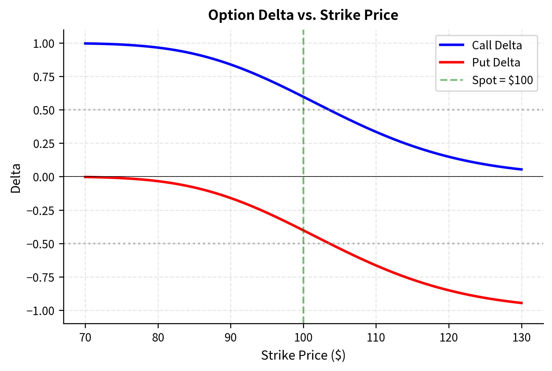
The plot illustrates how delta varies across different strike prices. For deep in-the-money calls (low strikes), delta approaches 1, indicating the option moves tick-for-tick with the stock. For deep out-of-the-money calls (high strikes), delta approaches 0. This curvature is captured by Gamma.
The next chapter provides comprehensive coverage of the Greeks, including their use in hedging strategies, portfolio risk management, and the dynamics of delta-hedged positions.
Extending to Dividend-Paying Stocks
The basic Black-Scholes formula assumes the stock pays no dividends. For stocks that pay a continuous dividend yield , we can modify the formula by replacing with . The intuition behind this adjustment is that dividend payments reduce the effective growth rate of the stock price. An investor who holds the stock receives dividends, but an investor who holds a call option does not. The option holder misses out on this cash flow, making the option less valuable.
The modified call pricing formula becomes:
where:
- : call option price
- : stock price
- : continuous dividend yield
- : time to expiration
- : cumulative standard normal CDF
- : strike price
- : risk-free rate
The factor discounts the stock price by the cumulative dividend yield over the option's life. Economically, this represents the fact that the stock will be worth less (by the amount of dividends paid out) at expiration than it would be without dividends. The call option, which only benefits from the terminal stock price, must account for this reduction.
The parameters and are modified as follows:
where:
- : stock price
- : strike price
- : risk-free rate
- : dividend yield
- : volatility
- : time to expiration
The key change is that replaces in the drift term. The effective growth rate of the stock under the risk-neutral measure is now the risk-free rate minus the dividend yield. This makes sense: dividends represent cash flowing out of the stock, reducing its expected appreciation rate.
where:
- : standardized moneyness term
- : volatility
- : time to expiration
The relationship between and remains unchanged; they still differ by exactly .
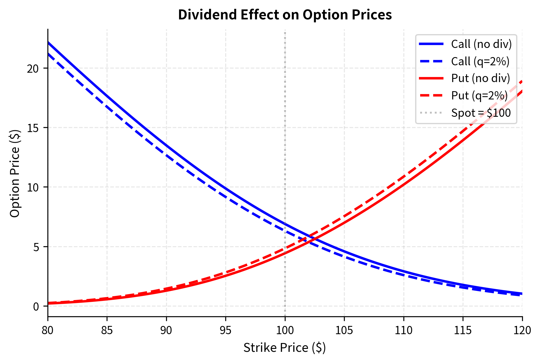
The dividend yield reduces the call value and increases the put value. Intuitively, dividends represent cash flows that benefit stockholders but not call option holders (who don't receive dividends until they exercise). Put holders, conversely, benefit from dividends because dividends reduce the stock price, making it more likely that the put will finish in-the-money.
The output shows that the dividend yield reduces the call price and increases the put price. This occurs because the dividend drops the expected stock price at expiration, making the call less likely to finish in-the-money and the put more likely.
Key Parameters
The key parameters for the Black-Scholes model with dividends are:
- : Current stock price.
- : Strike price.
- : Time to expiration.
- : Risk-free interest rate.
- : Volatility.
- : Continuous dividend yield. Represents cash flows paid to shareholders that option holders do not receive. Higher dividends decrease call values and increase put values.
Limitations of the Black-Scholes Model
While the Black-Scholes formula revolutionized option pricing and remains foundational, its assumptions limit its applicability in real markets.
The assumption of constant volatility is perhaps the most significant limitation. Empirical studies consistently show that volatility varies over time and exhibits clustering, with volatile periods tending to follow volatile periods. Moreover, when we examine implied volatilities from traded options, we find they vary systematically with strike price (the volatility smile) and with time to expiration (the term structure of volatility). These patterns directly contradict the constant volatility assumption and require more sophisticated models to explain.
The assumption of geometric Brownian motion implies that log-returns are normally distributed. However, as we discussed when studying stylized facts of financial returns, real asset returns exhibit heavy tails (more extreme moves than a normal distribution predicts) and negative skewness (large negative returns are more common than large positive returns). This means Black-Scholes systematically underprices options that pay off in extreme scenarios, particularly out-of-the-money puts that protect against market crashes.
The model assumes continuous trading with no transaction costs, allowing perfect delta hedging. In practice, transaction costs make continuous rebalancing impossible, and the discrete nature of trading introduces hedging errors. The model also assumes the ability to borrow and short-sell without restrictions at the risk-free rate, which may not hold for all market participants.
Finally, Black-Scholes prices European options only. American options, which can be exercised before expiration, require different techniques. Exotic options with path-dependent payoffs or multiple underlying assets also need more general pricing methods, which we'll cover in subsequent chapters on binomial trees and Monte Carlo simulation.
Despite these limitations, Black-Scholes remains the benchmark model. Market participants quote implied volatilities (the volatility that makes Black-Scholes match market prices) rather than dollar prices, using Black-Scholes as a translation device. Understanding Black-Scholes deeply is essential before moving to more complex models.
Summary
The Black-Scholes formula for European option pricing is:
where:
- : call option price
- : stock price
- : cumulative standard normal CDF
- : standardized moneyness terms
- : strike price
- : risk-free interest rate
- : time to expiration
where:
- : put option price
- : strike price
- : risk-free interest rate
- : time to expiration
- : cumulative standard normal CDF
- : standardized moneyness terms
- : stock price
Key insights:
-
Solution from the PDE: The Black-Scholes formula arises from solving the Black-Scholes PDE (derived in the previous chapter) subject to the option's terminal payoff condition. The solution involves transforming the PDE to the heat equation and applying the risk-neutral valuation principle.
-
Probabilistic interpretation: is the risk-neutral probability that the option expires in-the-money, while relates to the expected stock price conditional on exercise under a different measure.
-
Five inputs, one unknown: The formula takes five parameters: stock price, strike, time to expiration, interest rate, and volatility. Only volatility must be estimated, making it the central challenge in option pricing.
-
Monotonic relationships: Call prices increase with stock price, volatility, and interest rate, and decrease with strike price. Put prices exhibit the opposite relationships for stock price and rate. Both option types increase with volatility and time.
-
The Greeks: Delta, Gamma, Theta, Vega, and Rho quantify sensitivity to the five inputs. These partial derivatives are essential for hedging and risk management, which we'll explore comprehensively in the next chapter.
-
Model limitations: Constant volatility, normally distributed returns, continuous trading, and European exercise only are assumptions that don't perfectly match reality. Understanding these limitations guides when to use more sophisticated models.
The Black-Scholes formula, despite its simplifying assumptions, provides the foundation for all of options theory. The concepts of delta hedging, implied volatility, and risk-neutral pricing that emerge from this framework underpin modern derivatives markets.
Quiz
Ready to test your understanding? Take this quick quiz to reinforce what you've learned about the Black-Scholes formula and European option pricing.

Comments