

Learn how IA3 adapts large language models by rescaling activations with minimal parameters. Compare IA3 vs LoRA for efficient fine-tuning strategies.

This article is part of the free-to-read Language AI Handbook
Choose your expertise level to adjust how many terms are explained. Beginners see more tooltips, experts see fewer to maintain reading flow. Hover over underlined terms for instant definitions.
IA3
While LoRA achieves impressive parameter efficiency by learning low-rank updates to weight matrices, researchers at Google asked a simpler question: what if you could adapt the model by learning to rescale existing activations instead of modifying the weights? This led to IA3 (Infused Adapter by Inhibiting and Amplifying Inner Activations), which achieves even greater parameter efficiency than LoRA. IA3 learns element-wise rescaling vectors instead of low-rank matrix decompositions.
The core idea is simple: instead of learning like LoRA, IA3 learns a vector that scales activations through element-wise multiplication. LoRA might require thousands of parameters per adapted layer. IA3 needs only parameters, where is the hidden dimension. For a 7-billion parameter model, you can adapt with just 0.01% of the original parameters while still achieving competitive performance on many tasks.
IA3 was introduced by Liu et al. in their 2022 paper "Few-Shot Parameter-Efficient Fine-Tuning is Better and Cheaper than In-Context Learning." The method emerged from studying how to make parameter-efficient fine-tuning work well in few-shot scenarios where minimal training data is available. The authors discovered that the multiplicative nature of IA3's rescaling vectors, which provides better inductive biases for few-shot learning than additive methods like LoRA, improved performance.
The IA3 Formulation
To understand IA3, let's first establish how standard transformer layers compute their outputs. This foundation shows where IA3 intervenes and why those points were chosen. In multi-head attention, the model computes queries, keys, and values through linear projections:
where:
- : the query matrix
- : the key matrix
- : the value matrix
- : the input sequence matrix ()
- : the query projection matrix ()
- : the key projection matrix ()
- : the value projection matrix ()
- : the sequence length
- : the model hidden dimension
The attention output then feeds into a feed-forward network with projections and .
The key question: where should we insert our adaptation mechanism and why? IA3 targets keys, values, and feed-forward intermediate activations. Queries determine what information a position is looking for. Keys and values determine what information is available to be found and retrieved. By rescaling keys, you can change which tokens appear relevant to a query. By rescaling values, you can modify what information gets aggregated when attention weights are applied. By rescaling feed-forward activations, you can adjust which learned features are emphasized in the transformation pipeline.
IA3 modifies these computations by introducing learned rescaling vectors that multiply the keys, values, and feed-forward intermediate activations. Specifically, IA3 learns three vectors:
- for rescaling keys
- for rescaling values
- for rescaling feed-forward activations
The modified computations become:
where:
- : the rescaled key matrix
- : the rescaled value matrix
- : the learned rescaling vector for keys
- : the learned rescaling vector for values
- : the standard key projection of the input
- : the standard value projection of the input
- : element-wise multiplication (broadcast across the sequence dimension)
Notice how simple this formulation is. The original projection produces a matrix where each row represents a token's key vector. The rescaling vector then multiplies each dimension of every key vector by the same factor. If , then the -th dimension of every key in the sequence gets doubled. If , the -th dimension gets halved. This uniform rescaling across all positions allows IA3 to learn which aspects of the key representation matter most for your downstream task.
For feed-forward layers with intermediate activation where is the activation function, IA3 applies:
where:
- : the rescaled intermediate activation
- : the learned rescaling vector
- : the original intermediate activation
- : element-wise multiplication
- : the activation function (e.g., GELU)
- : the first feed-forward projection matrix
The feed-forward rescaling operates on a particularly interesting point in the computation. After the input passes through the first projection and nonlinearity, the intermediate representation exists in a higher-dimensional space (typically 4 times the hidden dimension). This expanded space contains specialized features that the model learned during pretraining. By rescaling these intermediate features, IA3 can effectively turn specific computational pathways on or off, amplifying features relevant to the current task while suppressing those that might introduce noise.
The Hadamard product, , performs element-wise multiplication between vectors or matrices of the same shape. For vectors , the result is for each element .
The key insight is that these rescaling operations don't change the weight matrices at all. Instead, they learn to amplify or inhibit specific dimensions of the activation space. When , the -th dimension is amplified. When , it's inhibited. When , the original behavior is preserved (no rescaling). This creates a natural interpretation: the model learns a "volume control" for each dimension of its internal representations, turning up dimensions that help with the task and turning down dimensions that don't contribute or that introduce interference.
Understanding Learned Rescaling Vectors
Why does rescaling activations work for task adaptation? The intuition comes from understanding what pretrained models have already learned. During pretraining, models develop rich representations where different dimensions encode different information types, some capture syntactic relationships, others capture semantic meanings, and still others encode task-specific patterns. These dimensions emerge organically from the pretraining objective, with the model learning to distribute information across available capacity in ways that best predict the next token.
When fine-tuning for a specific downstream task, you often just need to reweight which aspects of the existing representations matter most rather than learning entirely new computations. IA3's rescaling vectors learn exactly this reweighting. Think of it as a spotlight: the pretrained model has learned to notice many different features of the input, and IA3 learns which of those features deserve attention for the current task.
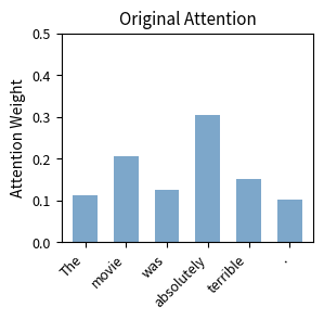
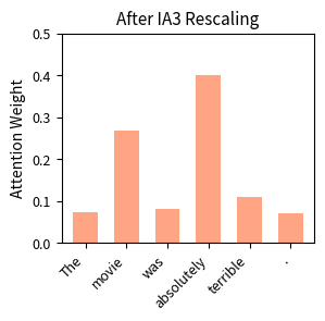
Consider a concrete example, adapting a pretrained model for sentiment analysis. The model already understands language and has dimensions that respond to emotional words, negation patterns, and intensifiers. IA3 learns which of these existing capabilities to emphasize. It might learn to amplify dimensions sensitive to sentiment-bearing words while dampening dimensions focused on factual content. A dimension that fires strongly when processing numerical quantities might be suppressed because such information rarely matters for sentiment. Meanwhile, a dimension that activates for words like "wonderful," "terrible," or "disappointing" might be amplified because these words carry crucial sentiment signals.
Mathematically, we can understand IA3 as learning a diagonal matrix transformation. If we define as the diagonal matrix with on the diagonal, then:
where:
- : the rescaled key matrix
- : the rescaling vector
- : the input sequence
- : the pretrained projection matrix
- : the diagonal matrix formed from ()
- : element-wise multiplication
This reformulation reveals something important about IA3's expressivity. A diagonal matrix can only stretch or compress coordinates independently. It cannot rotate the space or create new directions. This shows that IA3 is equivalent to right-multiplying the key projection by a diagonal matrix. Compared to LoRA's full low-rank update , IA3's diagonal update is far more constrained but requires dramatically fewer parameters. The low-rank matrices in LoRA can express rotations, projections onto subspaces, and more general linear transformations. IA3 sacrifices this flexibility for extreme efficiency, betting that the existing coordinate system is already well-suited to the task and only needs adjustment in magnitude.
Initialization Strategy
IA3 initializes all rescaling vectors to ones: . This initialization is crucial because it means the model starts with exactly the same behavior as the pretrained model. On the very first forward pass before any training occurs, every activation passes through unchanged. During training, the vectors gradually shift away from unity to adapt the model. Each dimension can move in its own direction based on task-specific gradients.
This contrasts with LoRA's initialization, where the matrix is initialized with small random values and with zeros. Both approaches ensure your adapted model starts equivalent to the pretrained model, but they arrive there through different means. LoRA achieves equivalence by making the adaptation term zero (since ), while IA3 achieves it by making the multiplication an identity operation (since ). The philosophical difference is subtle but meaningful: LoRA starts from "no change" while IA3 starts from "change by factor of one."
Parameter Count Analysis
Let's quantify exactly how parameter-efficient IA3 is. Understanding these numbers helps you decide which method to use in resource-constrained scenarios. For a standard transformer layer with hidden dimension and feed-forward dimension (typically ), IA3 introduces:
- parameters for (key rescaling)
- parameters for (value rescaling)
- parameters for (feed-forward rescaling)
The total per layer is . For a typical configuration where :
where:
- : the hidden dimension of the model
- : the feed-forward dimension (typically )
- : parameters for key and value rescaling vectors ()
- : parameters for the feed-forward rescaling vector (), assuming
This linear scaling with hidden dimension is remarkably gentle. As models grow larger, their hidden dimensions increase, but IA3's parameter count grows only proportionally, not quadratically as the original weights do.
Compare this to LoRA. For LoRA with the same components (keys, values, and feed-forward layers) and rank :
where:
- : the rank of the adaptation
- : the hidden dimension
- : the feed-forward dimension ()
- : parameters per attention matrix (keys, values)
- : parameters per feed-forward matrix
The crucial difference is the factor of in LoRA's count. Even at rank 1, LoRA requires more parameters than IA3. At typical ranks used in practice, the gap becomes substantial.
For LoRA with typical rank and hidden dimension , here's the comparison:
- LoRA: parameters per layer
- IA3: parameters per layer
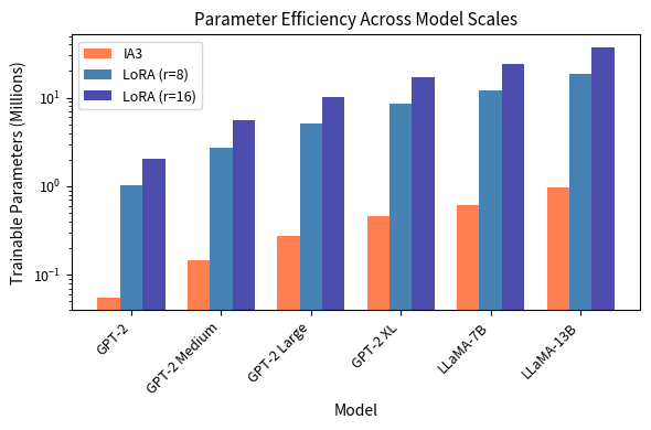
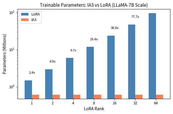
IA3 requires roughly 2.3r times fewer parameters than LoRA in general (approximately 19 times fewer at rank 8).
For LLaMA-7B, IA3 requires just over 600,000 trainable parameters, while LoRA with rank 8 needs approximately 12 million. This extreme efficiency makes IA3 particularly attractive for scenarios where memory is severely constrained or when you need to store many task-specific adaptations.
Implementation
Let's implement IA3 to see how the rescaling mechanism works in practice. We'll create IA3-adapted versions of attention and feed-forward layers.
The key lines are K = self.l_k * K and V = self.l_v * V, which perform simple element-wise multiplication that distinguishes IA3-adapted attention from standard attention. The rescaling vectors l_k and l_v start at ones, preserving the original model behavior, then learn to amplify or suppress specific dimensions during training.
The feed-forward implementation follows the same pattern. The rescaling happens after the first linear projection and activation function, allowing IA3 to learn which intermediate features are most relevant for the downstream task.
The ia3_parameters method provides convenient access to just the trainable rescaling vectors, making it easy to set up optimizers that only train these parameters.
With a 512-dimensional model and 2048-dimensional feed-forward, IA3 adds just 3,072 trainable parameters to a block that contains over 2 million frozen parameters. This demonstrates the dramatic efficiency gains you can achieve.
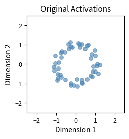
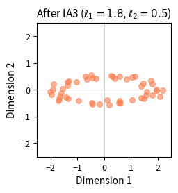
Visualizing Learned Rescaling
Let's visualize how rescaling vectors change from their initial uniform values to build intuition about what IA3 learns.
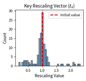
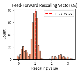
The histograms show how learned rescaling vectors deviate from their initial uniform values of 1.0. Some dimensions are amplified well above 1.0, while others are suppressed toward 0. This selective amplification and inhibition is how IA3 adapts the pretrained model's behavior without changing any of the original weights.
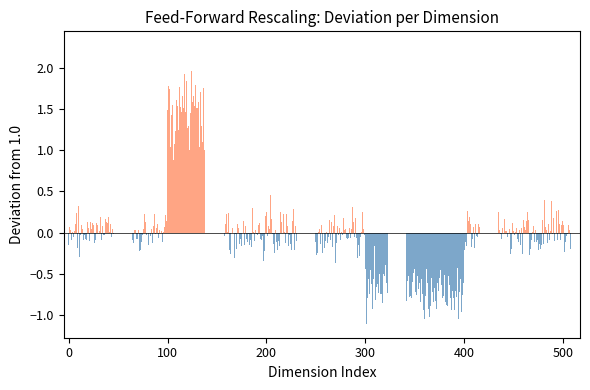
This dimension-wise view reveals that IA3 learns structured patterns. Consecutive dimensions often show similar rescaling behavior, suggesting the model discovers meaningful groups of features to amplify or suppress together.
IA3 vs LoRA: A Detailed Comparison
Having covered LoRA in previous chapters and now IA3, let's compare these two PEFT methods across several dimensions.
Mathematical Formulation
The fundamental difference lies in how each method parameterizes the adaptation. Understanding this difference mathematically helps clarify when each approach is most appropriate.
LoRA learns an additive low-rank update:
where:
- : the adapted weight matrix
- : the frozen pretrained weights
- : the scaling factor
- : the rank
- : the low-rank output matrix ()
- : the low-rank input matrix ()
- : the input dimension
- : the output dimension
The additive nature of LoRA means it learns to supplement the original weight matrix. The product represents a new linear transformation added to what the model originally computed. This addition happens in weight space, before any activations are computed.
IA3 learns a multiplicative diagonal scaling:
where:
- : the scaled activation
- : the learnable rescaling vector ()
- : the input activation
- : element-wise multiplication
IA3's multiplicative intervention happens in activation space, after the original computation but before the result is used downstream. Rather than changing what gets computed, IA3 changes how much of each computed quantity flows forward in the network.
LoRA modifies what the model computes by adding new terms to weight matrices. IA3 modifies how much the model uses what it already computes by rescaling activations. Choose between them based on your constraints and task requirements.
Parameter Efficiency
Even at rank 1, LoRA requires about 4 times more parameters than IA3. At the commonly used rank 8, LoRA needs approximately 50 times more parameters. This dramatic difference stems from IA3 needing only parameters per adapted component versus LoRA's parameters.
Expressivity vs Efficiency Tradeoff
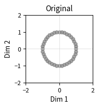
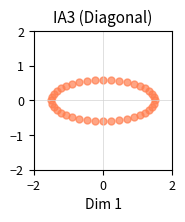
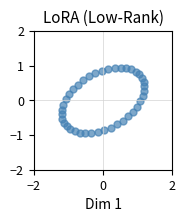
IA3's extreme efficiency comes with reduced expressivity. LoRA can learn arbitrary low-rank updates to weight matrices, while IA3 can only learn diagonal scaling. This limitation means IA3 cannot change the direction of computations, only their magnitude.
Consider what each method can express geometrically. LoRA's update can rotate, scale, and project the input in any direction within a rank- subspace. IA3's diagonal scaling can only stretch or compress along the existing coordinate axes. If you imagine the model's representations as points in a high-dimensional space, LoRA can learn to rotate that space into a new orientation. IA3 can only stretch or squeeze it along the original axes.
Despite this limitation, IA3 often performs surprisingly well, particularly in few-shot scenarios. The authors of the original paper hypothesize that pretrained models already contain most of the computational machinery needed for downstream tasks. What fine-tuning needs to learn is mainly which existing computations to emphasize, which is exactly what IA3 provides. This hypothesis suggests that the geometry learned during pretraining is already well-suited to many tasks, and adaptation is more about emphasis than restructuring.
Training Dynamics
The two methods also differ in their training dynamics. LoRA uses standard weight decay regularization on the and matrices. IA3 applies no explicit regularization to rescaling vectors, but the multiplicative nature of the adaptation provides implicit regularization.
When IA3's rescaling values approach zero, they effectively disable entire dimensions. This creates a natural form of feature selection where unimportant dimensions get suppressed. LoRA, being additive, doesn't have this same dynamic. Setting to zero means no adaptation, not suppression of existing computations.
Merging Behavior
Both LoRA and IA3 can merge their adaptations into the base model weights for efficient inference. For LoRA, add the low-rank product to the original weights: . For IA3, the merging is multiplicative.
When the rescaling is applied after a linear projection, IA3 can merge by right-multiplying the weight matrix:
where:
- : the merged weight matrix
- : the original weight matrix
- : the diagonal matrix of rescaling factors
- : the vector of learned rescaling values
This modifies each column of by its corresponding rescaling factor. The merged model then runs with no additional overhead, just like LoRA.
When to Choose Each Method
Based on this analysis, use these guidelines for choosing between IA3 and LoRA:
Choose IA3 when:
- Memory is extremely constrained
- You must store many task-specific adaptations
- Working in few-shot scenarios (10-1000 examples)
- The downstream task is similar to pretraining
- Training speed is critical (fewer parameters means faster updates)
Choose LoRA when:
- You need higher model expressivity
- The downstream task differs significantly from pretraining
- You have sufficient training data to learn more complex adaptations
- You need fine-grained control over adaptation rank per layer
IA3 with PEFT Library
The Hugging Face PEFT library provides a convenient implementation of IA3 that integrates seamlessly with transformers models.
The PEFT library handles all the complexity of identifying which modules to adapt and wrapping them with IA3 rescaling. The target_modules parameter specifies which attention components to adapt (keys and values), while feedforward_modules identifies feed-forward layers that get the rescaling.
Each adapted layer receives its own set of rescaling vectors. The IA3 vectors are named with ia3_l in their parameter names, making them easy to identify.
Limitations and Impact
IA3's extreme parameter efficiency comes with meaningful limitations. The most significant limitation is expressivity—IA3 can only rescale existing activations and cannot learn fundamentally new computations. If your downstream task requires capabilities not present in the pretrained model, IA3 may underperform compared to LoRA, which can add new computational pathways. This limitation manifests most clearly when the downstream task distribution differs substantially from the pretraining data.
Another limitation is the lack of a tunable capacity parameter. LoRA provides the rank hyperparameter that allows you to trade off between efficiency and expressivity. IA3 has no such tuning option. You get exactly parameters per rescaling vector, no more, no less. While this simplifies hyperparameter search, it also means you cannot easily scale up IA3's capacity when your task demands it.
The multiplicative nature of IA3 also creates potential training instabilities. If rescaling values grow too large during training, they can cause exploding activations. Conversely, values approaching zero can create vanishing gradient problems. You can manage these issues with careful learning rate selection and gradient clipping. However, IA3 requires more attention than LoRA.
Despite these limitations, IA3 has had a significant impact on the PEFT landscape. It demonstrated that the field's assumptions about necessary adaptation capacity were often too conservative. Many tasks that practitioners thought required LoRA or full fine-tuning actually work well with simple rescaling. This insight has informed the development of subsequent methods and encouraged exploration of other minimal-parameter approaches.
IA3 has proven particularly valuable for few-shot learning scenarios. The original paper showed that IA3 outperformed in-context learning (using examples in the prompt) while using orders of magnitude less inference compute. This positioned IA3 as an efficient alternative to few-shot prompting when you need to perform the same task repeatedly.
The method has also influenced thinking about what fine-tuning actually learns. IA3's success suggests that pretrained language models contain most needed capabilities and adaptation primarily reweights existing features rather than learning new ones. This perspective has implications for how we design both pretraining objectives and fine-tuning strategies.
Summary
IA3 offers a simple approach to parameter-efficient fine-tuning: instead of learning weight updates like LoRA, it learns to rescale existing activations. By learning vectors , , and that multiply keys, values, and feed-forward activations respectively, IA3 adapts pretrained models with dramatically fewer parameters than other PEFT methods.
Key insights from IA3 include:
- Rescaling as adaptation: Learned element-wise multiplication can effectively adapt pretrained models by amplifying relevant dimensions and suppressing irrelevant ones
- Extreme efficiency: IA3 requires roughly parameters per transformer layer compared to LoRA's , often achieving 10-50x parameter reduction
- Multiplicative dynamics: Starting from uniform rescaling (all ones) and learning deviations provides strong inductive biases for few-shot learning scenarios
- Limited expressivity: IA3 diagonal adaptation cannot learn rotations or projections, only magnitude changes along existing axes
In the next chapter on Prefix Tuning, we explore a different approach: prepending learned embeddings to the input sequence. This contrasts with IA3, which modifies how activations flow through the model. This technique offers yet another perspective on how minimal interventions can effectively adapt large language models.
Quiz
Ready to test your understanding? Take this quick quiz to reinforce what you've learned about IA3 and its approach to parameter-efficient fine-tuning.

Comments