

Explore how in-context learning emerges in large language models. Learn about scale thresholds, ICL vs fine-tuning, induction heads, and meta-learning.
This article is part of the free-to-read Language AI Handbook
Choose your expertise level to adjust how many terms are explained. Beginners see more tooltips, experts see fewer to maintain reading flow. Hover over underlined terms for instant definitions.
In-Context Learning Emergence
In Part XVIII, we introduced in-context learning (ICL) as a remarkable capability of large language models: the ability to perform new tasks simply by observing a few demonstrations in the prompt, without any gradient updates. But when we introduced ICL, we treated it as a feature of GPT-3 and its successors. What we didn't fully address was the mystery of when and how this capability appears.
ICL doesn't exist at small scales. Train a language model with 100 million parameters on the same data, with the same architecture, and you'll find something peculiar. The model doesn't learn from examples in the prompt. It will generate text, predict next tokens, and even produce coherent sentences, but showing it examples of a task at inference time has little effect on its behavior. Then, somewhere between 1 billion and 100 billion parameters, something changes. The model starts using those examples. It begins to generalize from demonstrations it has never seen during training to produce correct outputs for novel inputs.
This emergence of in-context learning represents one of the most consequential transitions in the scaling of language models. It transformed LLMs from pattern-matching text generators into flexible few-shot learners, fundamentally changing how we interact with AI systems. Understanding when this transition occurs, how it scales compared to traditional fine-tuning, and what mechanisms might explain it remains an active area of research with significant implications for both theory and practice.
ICL Emergence Curves
The emergence of in-context learning follows characteristic patterns that researchers have documented across multiple model families and scales. Unlike smooth improvements in perplexity or basic language modeling metrics, ICL ability appears relatively suddenly as models cross certain scale thresholds.
The Scale Threshold Phenomenon
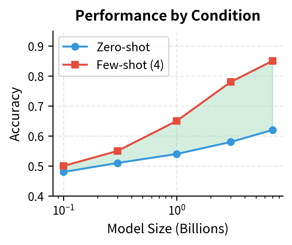
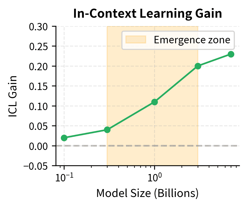
Early investigations by Brown et al. with GPT-3 revealed that in-context learning performance improves dramatically with model size, but this improvement is highly non-linear. On many tasks, models below approximately 1 billion parameters show essentially random performance when given few-shot examples, while models above 10-100 billion parameters achieve substantial accuracy gains from the same demonstrations.
The emergence curve for ICL typically follows a pattern with several distinct phases:
- Random baseline phase: Small models (typically <1B parameters) show no meaningful improvement from in-context examples. Performance remains near chance regardless of demonstration quality or quantity.
- Transition phase: Models in an intermediate range begin showing some sensitivity to demonstrations, but performance is unstable and task-dependent.
- Competent phase: Larger models consistently leverage demonstrations, with performance scaling log-linearly with both model size and number of examples.
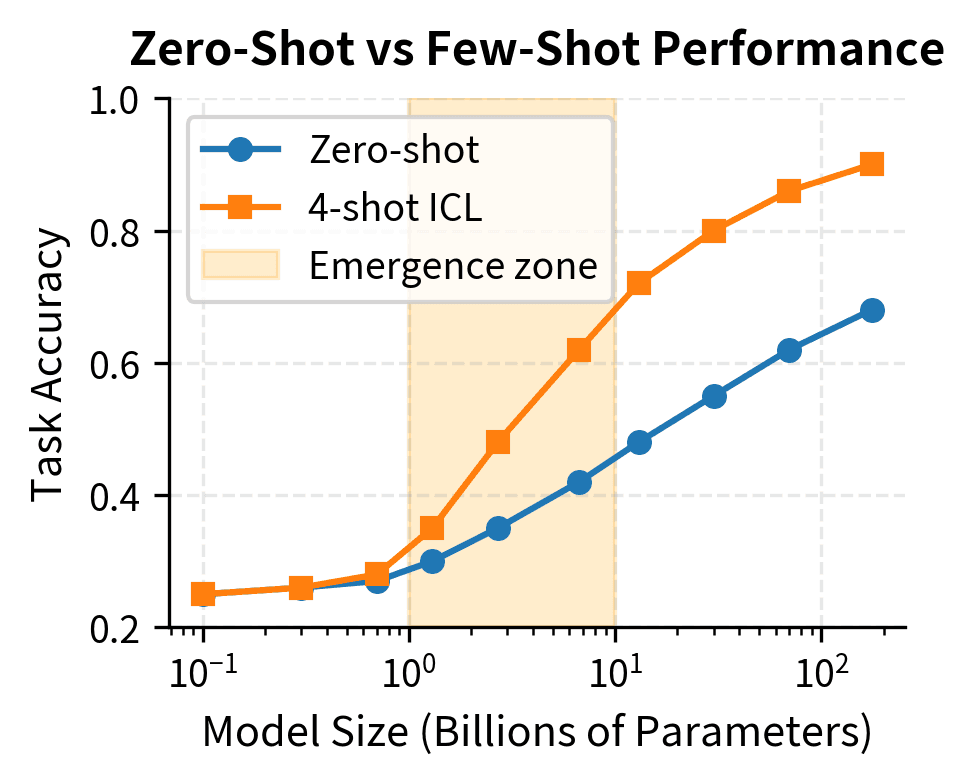

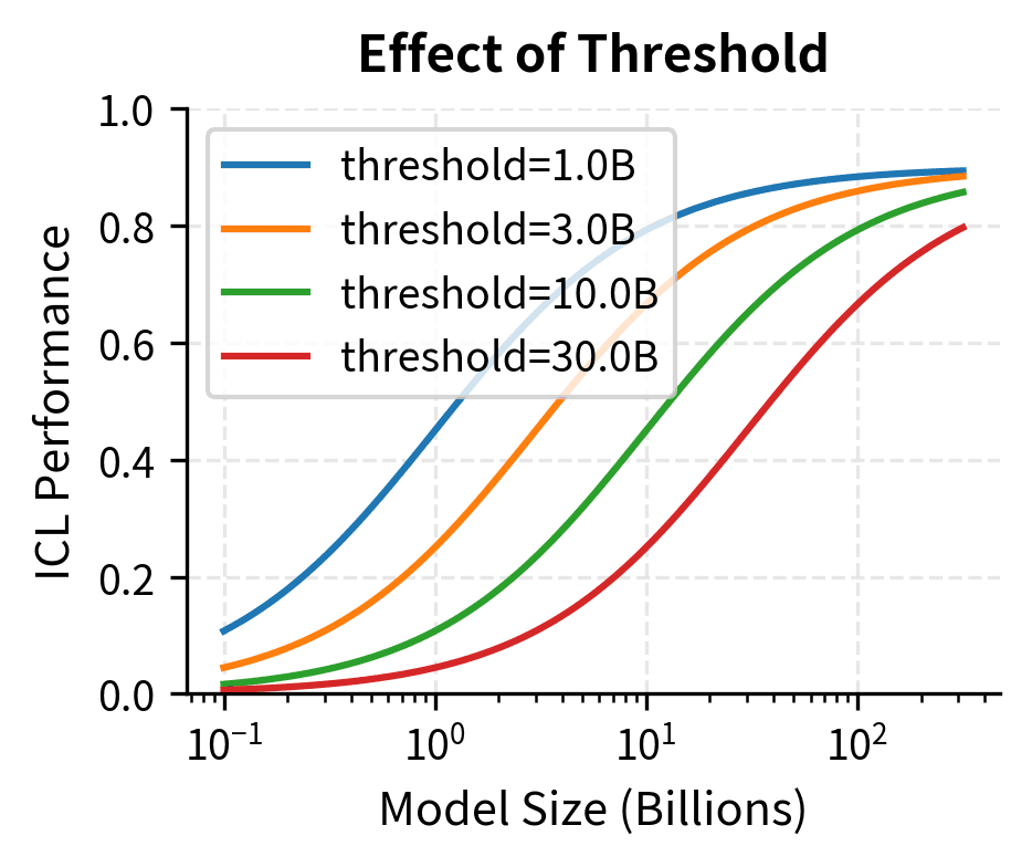
This visualization reveals the characteristic S-curve of ICL emergence. Below 1B parameters, demonstrations provide almost no benefit. Between 1B and 10B parameters, ICL ability emerges rapidly. Above 10B parameters, models reliably exploit few-shot examples, though the marginal gains continue to compound with scale.
Task-Dependent Emergence Thresholds
Not all tasks exhibit identical emergence thresholds. Some capabilities emerge earlier than others, creating a hierarchy of ICL difficulty:
Early-emerging tasks (emerge at smaller scales) typically include:
- Simple pattern completion
- Basic translation of common language pairs
- Sentiment classification with clear signals
- Factual question answering about high-frequency knowledge
Late-emerging tasks (require larger scales) include:
- Multi-step arithmetic
- Abstract reasoning and analogy
- Low-resource language translation
- Tasks requiring world knowledge integration
This task hierarchy suggests that ICL emergence isn't a single phenomenon but rather a spectrum of capabilities that unlock progressively with scale. Wei et al. (2022) documented this pattern systematically, showing that the emergence threshold varies by more than an order of magnitude across different task types.
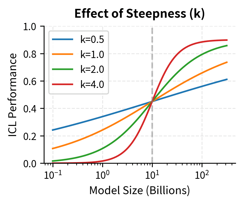
The sigmoid emergence function captures a fundamental insight about how capabilities develop in neural networks. Rather than appearing gradually, ICL ability transitions rapidly once the model crosses a critical scale threshold. The function operates in log-space because the relationship between model size and capability is multiplicative rather than additive. Doubling the parameters doesn't add a fixed amount of capability, but rather multiplies the model's effective capacity. The threshold parameter marks the inflection point where the model transitions from having essentially no ICL ability to having substantial capability. The steepness parameter controls how abrupt this transition is; higher values produce sharper phase transitions, while lower values create more gradual emergence curves. This mathematical formulation allows researchers to precisely characterize and compare emergence patterns across different tasks and model families.
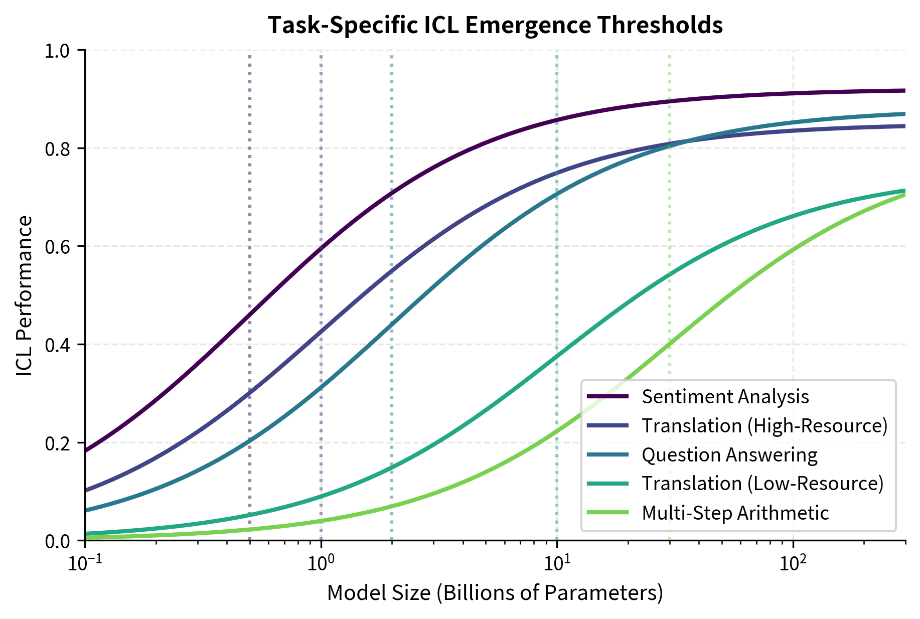
The emergence curves reveal a clear hierarchy: sentiment analysis reaches 50% of maximum performance at just 0.5B parameters, while multi-step arithmetic requires approximately 30B parameters to achieve the same relative capability. This 60-fold difference in emergence thresholds demonstrates that ICL is not a monolithic capability but a family of skills with vastly different computational requirements.
Training Data and Compute
Scale alone doesn't fully determine ICL emergence. The Chinchilla scaling laws we covered in Part XXI showed that optimal model performance requires balancing model size with training data quantity. Given a fixed compute budget, there exist optimal allocations for both model size and training data:
where:
- : the optimal number of model parameters for a given compute budget
- : the optimal number of training tokens
- : the total compute budget (measured in FLOPs)
- : denotes proportionality (the quantities scale together but may differ by a constant factor)
The exponent of indicates square-root scaling: if you double your compute budget, both the optimal model size and optimal data quantity should increase by a factor of . This square-root relationship ensures neither parameter count nor data becomes a bottleneck. This balance also affects ICL emergence.
To understand why this relationship matters for ICL emergence, consider what happens when you deviate from optimal allocation. If you invest all additional compute into model size while keeping data fixed, the model becomes "undertrained." It has capacity it cannot effectively use because it hasn't seen enough diverse patterns during training. Conversely, if you invest all additional compute into data while keeping model size fixed, you create an "overexposed" model that has seen more patterns than it can represent. The Chinchilla insight is that both failure modes hurt performance, and the optimal path forward maintains a balance between the two. For ICL specifically, this means that raw parameter count is insufficient. The model must also have been trained on sufficient diverse data to develop the pattern recognition capabilities that underlie few-shot learning.
Research by Hoffmann et al. demonstrated that compute-optimal training can shift emergence curves leftward, meaning ICL capabilities appear at smaller model sizes when training is more efficient. A 10B parameter model trained optimally might exhibit ICL performance comparable to a 50B parameter model trained sub-optimally.
The quality and diversity of pre-training data also matters significantly. Models trained on more diverse corpora with greater task variety tend to develop stronger ICL abilities at equivalent scales. This observation connects to the meta-learning perspective we'll explore later in this chapter.
ICL vs Fine-tuning Scaling
A central question in the scaling of language models is how in-context learning compares to traditional fine-tuning as model size increases. Both approaches allow models to adapt to new tasks, but they do so through fundamentally different mechanisms.
Fine-tuning Scaling Behavior
Fine-tuning updates model weights through gradient descent on task-specific data. As we covered in Part XVII with BERT fine-tuning, this approach has been the standard method for adapting pre-trained models to downstream tasks. The scaling behavior of fine-tuning is relatively well understood.
Fine-tuning typically shows smooth, consistent improvements with scale. Even small models benefit substantially from fine-tuning on sufficient task-specific data. A 100M parameter model, while showing no ICL ability, can achieve strong performance when fine-tuned on thousands of labeled examples. The improvement from fine-tuning scales roughly log-linearly with both model size and data quantity.

The crossover point represents a significant milestone: beyond this scale, the efficiency of in-context learning begins to outweigh the benefits of traditional fine-tuning for low-data scenarios.
The Crossover Point
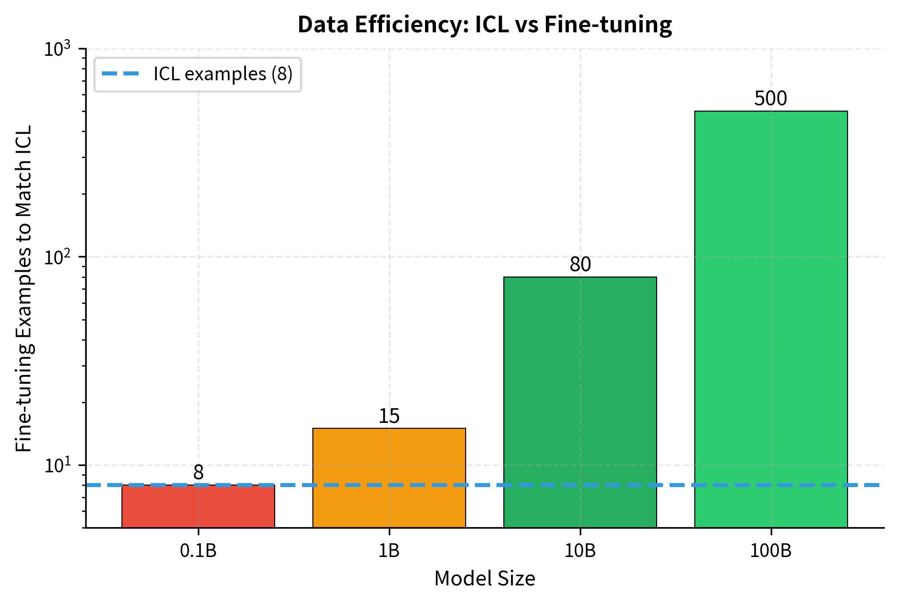
A striking phenomenon occurs as models scale: ICL eventually becomes competitive with, and can even surpass, fine-tuning despite using orders of magnitude fewer examples. This crossover has profound practical implications.
For small models, fine-tuning is strictly superior. A 1B parameter model fine-tuned on 100 examples dramatically outperforms the same model doing 8-shot ICL. But for large models (typically >30B parameters), 8-shot ICL can match or exceed fine-tuning with 100 examples. At the largest scales, ICL with a handful of demonstrations approaches the performance of fine-tuning with thousands of examples.
This crossover represents a qualitative shift in how we can use language models. Below the crossover, adapting models to new tasks requires collecting data, writing training pipelines, and running optimization. Above the crossover, you can achieve comparable results simply by writing a prompt.
Why the Scaling Difference?
The different scaling behaviors of ICL and fine-tuning reflect their fundamentally different mechanisms.
Fine-tuning explicitly optimizes model weights to minimize loss on task-specific data. This optimization process is reliable and well-understood. It works at any scale because gradient descent effectively finds task-relevant features in the model's representations. The limitation is that it requires many examples to adjust the millions or billions of parameters effectively.
ICL doesn't modify weights at all. Instead, it relies on the model's pre-trained ability to recognize patterns in the prompt and generalize from them. This ability is emergent, requiring sufficient model capacity and diverse pre-training to develop. Once it emerges, ICL can be remarkably data-efficient because the model has already learned general-purpose pattern recognition.
The practical implication is that ICL represents a shift from per-task adaptation to universal adaptation. A model with strong ICL abilities is essentially a general-purpose few-shot learner that can handle novel tasks without any task-specific training.
ICL Mechanism Hypotheses
Understanding how in-context learning works mechanistically remains an active research area. Several hypotheses have been proposed, offering different perspectives on what happens when a model processes demonstrations and then generalizes to new examples.
The Induction Head Hypothesis
Elhage et al. (2022) identified specific circuit structures called induction heads that appear to implement a form of in-context learning.
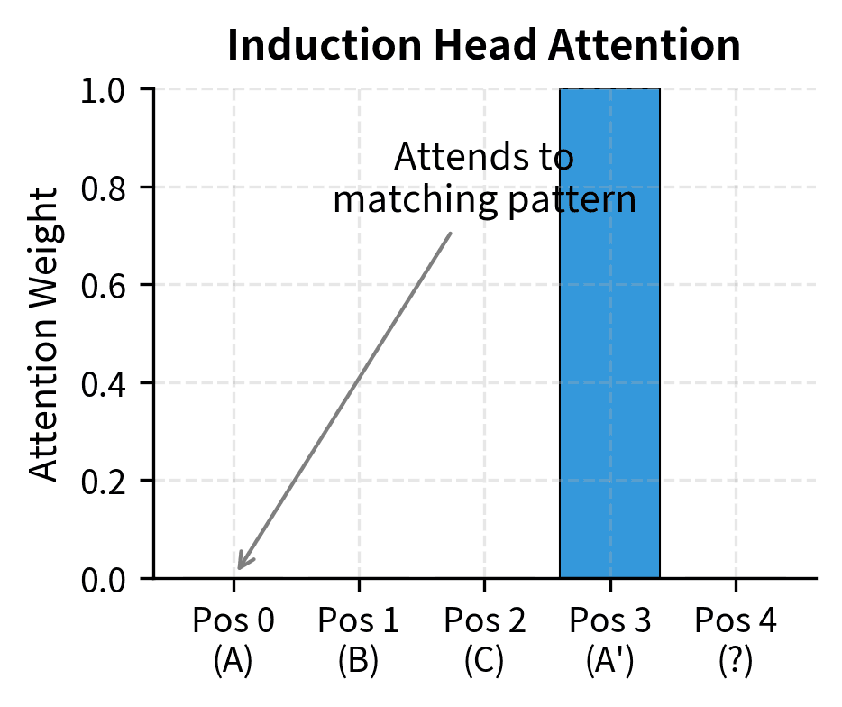
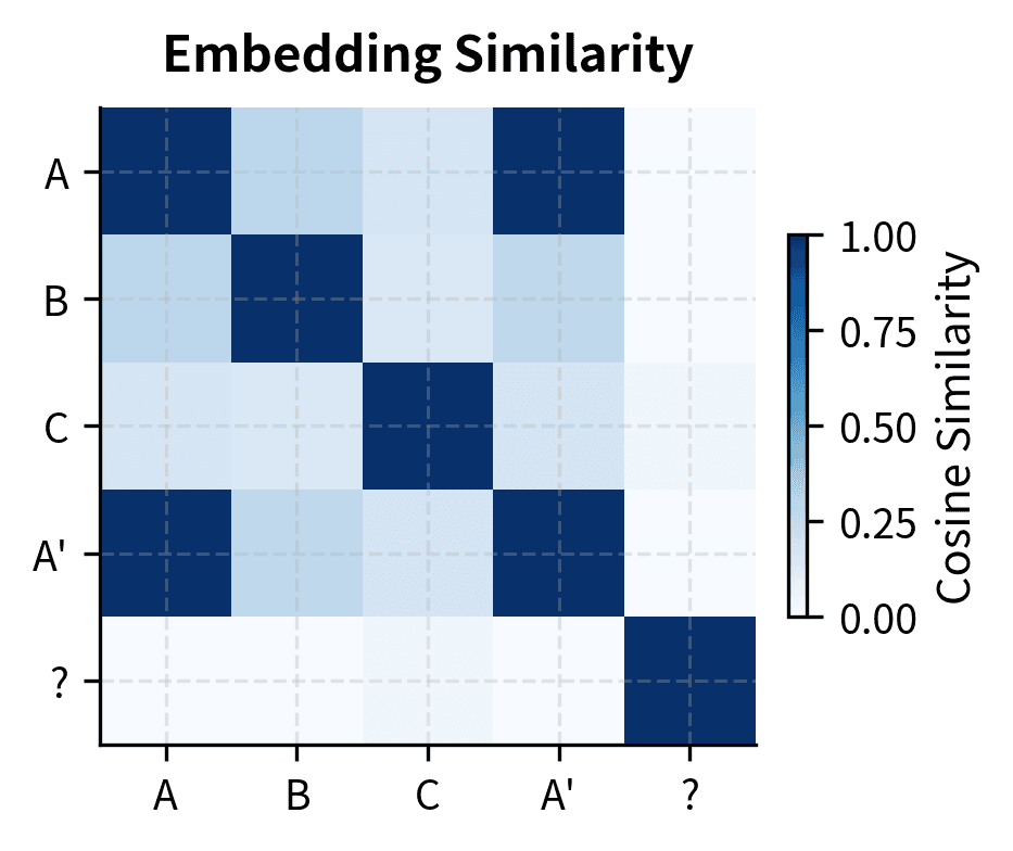
Induction heads are attention patterns that learn to copy tokens that followed similar contexts earlier in the sequence. They implement a primitive form of pattern completion: if the sequence contains "[A][B]...[A]", the induction head predicts [B] will follow.
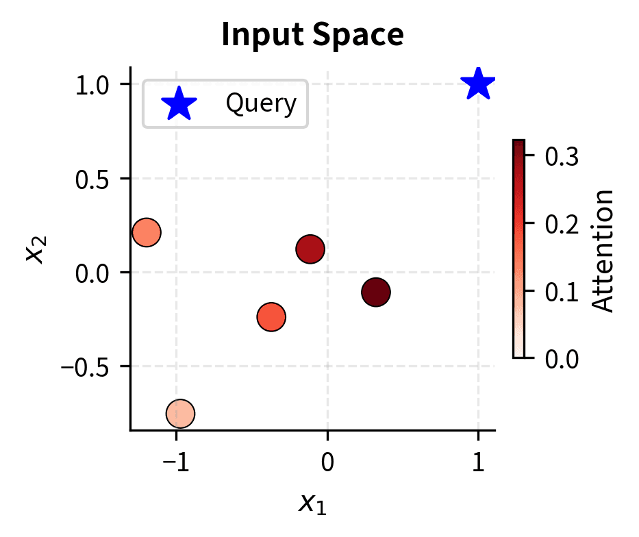
To understand why induction heads matter for ICL, consider what happens when you provide a model with demonstrations like "France → Paris, Germany → Berlin, Japan → ?" The model needs to recognize that the pattern "[Country] → [Capital]" has been established and that the same mapping should apply to the query. Induction heads provide exactly this capability: they scan the sequence for previous occurrences of similar patterns and copy the associated outputs. When the model encounters "Japan", an induction head can identify that similar country tokens were followed by capital city tokens, enabling it to predict "Tokyo" even without explicit training on this particular mapping.
Induction heads emerge during training, and their formation coincides with a sudden improvement in model performance. Researchers call this the "induction head phase transition." This transition typically occurs early in training and appears to be a prerequisite for more sophisticated ICL abilities.
The mechanism works through a two-step process that coordinates across multiple attention heads within the transformer architecture. First, an attention head identifies previous positions where a similar pattern occurred, effectively creating a lookup based on context similarity. Second, another attention head copies information from what followed that previous pattern, retrieving the associated continuation. This two-step coordination is what makes induction heads powerful. They implement a form of content-addressable memory where the model can retrieve relevant information based on contextual similarity rather than fixed position.
This circuit can explain simple ICL behaviors like learning a consistent mapping from inputs to outputs. If the model sees "[France → Paris], [Germany → Berlin], [Japan → ]", the induction head mechanism can recognize the pattern and predict "Tokyo" even if this specific mapping was never seen during training.
Gradient Descent in the Forward Pass
Akyürek et al. (2022) and von Oswald et al. (2023) suggest that transformers implementing ICL effectively perform gradient descent within the forward pass. Rather than learning by updating weights, the model's attention mechanisms simulate the optimization process that gradient descent would perform.
This perspective reframes in-context learning as implicit optimization. The demonstrations serve as a training set, and the attention layers compute something functionally equivalent to gradient updates on an internal linear model. This insight matters because it connects the mystery of ICL to the well-understood mathematics of optimization. If attention layers can implement gradient descent, then ICL is not magic. It is the model running a familiar learning algorithm using the computational substrate of attention.
The mathematical intuition is that a single attention layer computes a weighted combination of values, where the weights depend on query-key similarity:
where:
- : the query matrix, representing the current position's learned representation seeking information
- : the key matrix, representing what information each position offers
- : the value matrix, containing the actual information to be aggregated
- : the dimensionality of the key vectors, used for scaling to prevent dot products from growing too large
- : normalizes attention weights to sum to 1, creating a probability distribution over positions
The attention mechanism operates by first computing similarity scores between queries and keys through dot products. These raw scores are scaled by to maintain stable gradients. Without this scaling, large hidden dimensions would produce extreme dot products that make softmax outputs nearly one-hot, hampering gradient flow during training. The softmax then converts these scaled similarities into a proper probability distribution, determining how much each position contributes to the output. Finally, the value vectors are weighted by these probabilities and summed, producing an output that aggregates information from positions deemed most relevant by the query-key matching.
With appropriate weight configurations, this operation can approximate a step of gradient descent on a linear regression objective. The key insight is that attention computes a weighted sum over values, and with the right setup, these weights can encode gradient information.
To see this connection, consider linear regression where we want to find weights that predict outputs from inputs. Gradient descent updates these weights by moving in the direction that reduces prediction error:
where:
- , : the weight vector after and before the update
- : the learning rate controlling step size
- : the number of training examples
- : the -th input feature vector
- : the -th target value
- : the prediction error, which measures how far off the current prediction is from the target
The gradient descent update adjusts the weights by adding a correction term that is proportional to the error scaled by the input and learning rate . Larger errors lead to larger corrections, and the input vector determines which weight dimensions get updated most. This is the core principle of supervised learning: use the discrepancy between prediction and truth to guide weight adjustments, with the input features determining the direction of adjustment in weight space.
The attention mechanism mirrors this structure. The query represents the current estimate (analogous to ), keys represent the training inputs (), and values encode the gradient information (error signals weighted by inputs). When the model processes demonstrations, the attention weights computed between the query position and demonstration positions can encode the gradient update that would be computed if we were training on those examples. The softmax normalization corresponds to how gradients are aggregated across training examples, and multiple attention layers can implement multiple gradient steps, refining the internal model iteratively.

This connection between attention and gradient descent provides a theoretical foundation for understanding why ICL works and why it emerges with scale. Larger models have more capacity to learn the weight configurations that implement this implicit optimization.
Task Recognition vs Task Learning
Another perspective distinguishes between two potential mechanisms: task recognition and task learning.
Task recognition proposes that during pre-training, the model learns many tasks implicitly. When given demonstrations at test time, the model doesn't learn a new task; instead, it recognizes which of its pre-existing capabilities to apply. The demonstrations serve as task specifiers rather than training data.
Task learning proposes that the model learns new input-output mappings from the demonstrations, even mappings it has never encountered during pre-training.
Research by Min et al. (2022) provided evidence for task recognition by showing that ICL performance remains robust when demonstration labels are randomized. This suggests models often recognize the task structure from the input format rather than learning the specific input-output mapping.
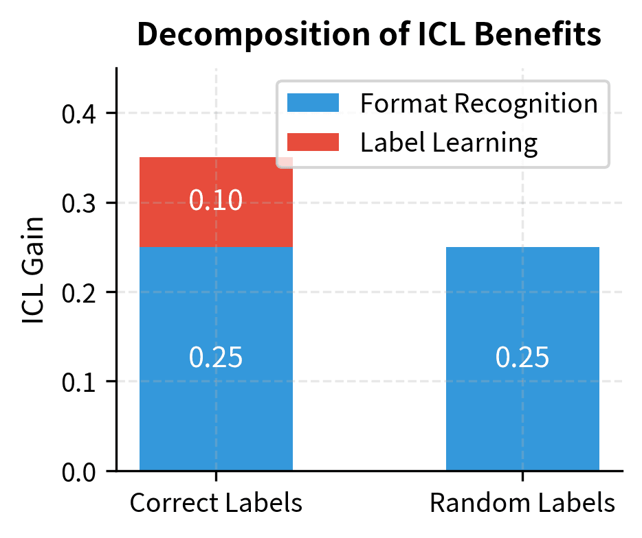
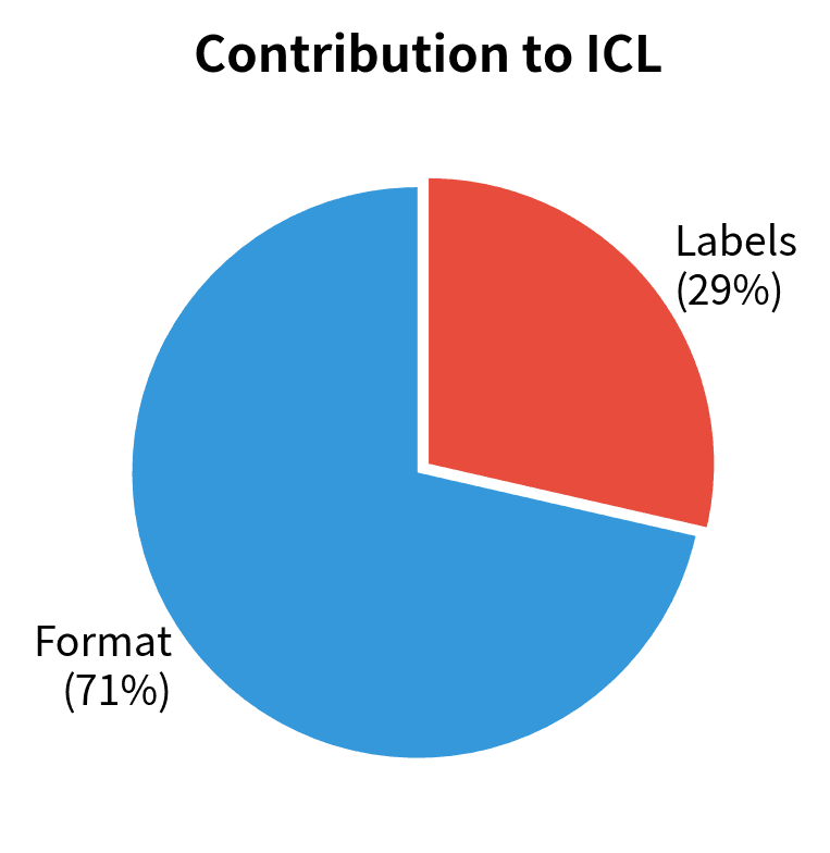
The reality likely involves both mechanisms. Task recognition explains why ICL works for tasks similar to pre-training distributions, while task learning (perhaps via the gradient descent mechanism) explains generalization to genuinely novel tasks.
ICL as Meta-Learning
Perhaps the most comprehensive framework for understanding in-context learning views it through the lens of meta-learning. This perspective explains both how ICL emerges and why it requires scale.
What is Meta-Learning?
Meta-learning, or "learning to learn," refers to algorithms that improve their learning ability through experience. Rather than learning a single task, a meta-learner learns how to learn new tasks quickly from limited data.
Traditional learning algorithms start fresh for each new task. Meta-learning algorithms leverage experience from previous tasks to accelerate learning on new ones. The classic formulation involves:
- An outer loop that learns across many tasks, updating how the model learns
- An inner loop that learns each specific task, using the meta-learned learning procedure
The goal is to develop a learning algorithm (not just a model) that can rapidly adapt to new tasks with minimal data. This is fundamentally different from traditional machine learning, where the algorithm is fixed (such as gradient descent) and only the model parameters change. In meta-learning, the learning procedure itself is learned, optimized to enable fast adaptation. The outer loop shapes the learning dynamics, while the inner loop applies those dynamics to individual tasks.
Pre-training as the Outer Loop
The meta-learning perspective on ICL views pre-training as an implicit outer loop that creates a general-purpose learning algorithm. During pre-training, the language model encounters billions of sequences containing implicit task structures. Each training sequence can be viewed as a mini-task, predicting what comes next given the context.
The diversity of pre-training data means the model implicitly sees many task distributions:
- Passages followed by summaries (summarization task)
- Questions followed by answers (QA task)
- Statements in one language followed by translations (translation task)
- Premises followed by conclusions (reasoning task)
By training on next-token prediction across this diverse distribution, the model learns to recognize task patterns and adapt its predictions accordingly. The model isn't just learning to predict text. It's learning to identify what kind of prediction is expected given the context.
This perspective illuminates why pre-training on diverse data is so crucial. Each time the model encounters a different type of text pattern, it must implicitly identify the genre, style, or task and adjust its predictions accordingly. Over billions of such encounters, the model develops a repertoire of "task programs" that it can flexibly invoke based on contextual cues. The pre-training objective, next-token prediction, provides the consistent supervision signal, but the underlying capability being developed is task recognition and adaptation.
Why Scale Enables Meta-Learning
The meta-learning framework explains why ICL requires scale. Effective meta-learning requires:
- Sufficient capacity to represent many different task-specific adaptation procedures
- Exposure to diverse tasks during training to learn robust meta-knowledge
- Representational flexibility to quickly adapt to new task contexts
Small models lack the capacity to maintain the rich meta-knowledge needed for flexible adaptation. They might learn to perform well on the average pre-training sequence, but they can't maintain the separate "programs" for different task types that enable ICL.
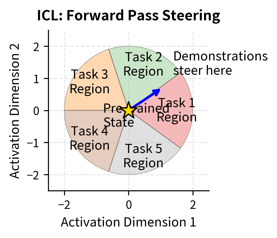
Large models, in contrast, develop what researchers sometimes call "task vectors" or "function vectors" within their representations. Different regions of the model's latent space correspond to different task types, and the demonstrations effectively steer the model toward the appropriate region.
The computational requirements for meta-learning exceed those for single-task learning. To learn a learning algorithm, the model must effectively encode not just how to perform each task, but also the meta-structure that allows rapid adaptation across tasks. This meta-structure includes pattern templates that capture task formats, input-output mapping functions that can be parameterized by demonstrations, and contextual routing mechanisms that direct processing based on task cues. Each of these components requires representational capacity, and they must all coexist without interfering with each other. This explains the scale threshold. Below a certain size, the model simply cannot represent all the components needed for flexible meta-learning.
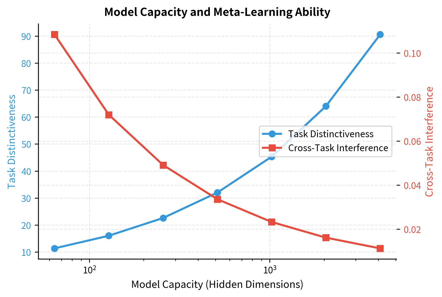
The visualization shows that larger model capacity leads to more distinct task representations and reduced cross-task interference. This separation is essential for the model to apply the right "program" when it recognizes a task from demonstrations.
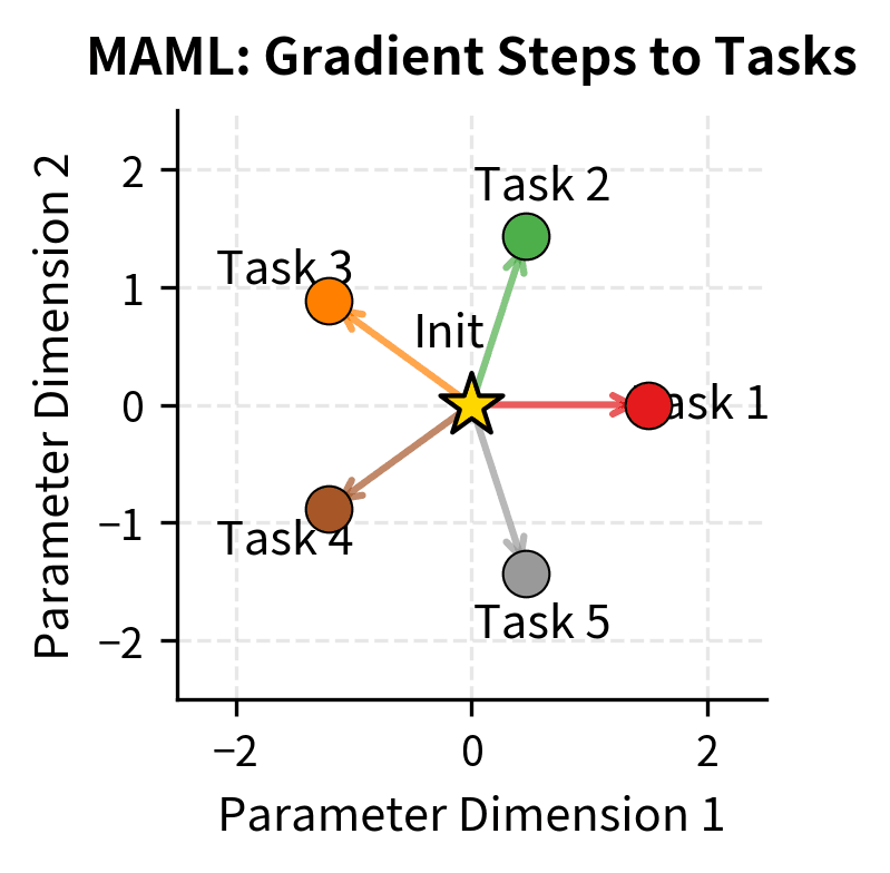
The MAML Connection
The meta-learning perspective connects ICL to established meta-learning algorithms like Model-Agnostic Meta-Learning (MAML). MAML explicitly trains models to be easily fine-tunable by optimizing for fast adaptation. The core idea is to find an initialization from which a single gradient step on any new task yields good performance. The MAML objective captures this through a bi-level optimization:
where:
- : the model's initial parameters (the meta-learned initialization we're optimizing)
- : the adapted parameters for task after one gradient step
- : a task sampled from the task distribution
- : the model parameterized by
- : the loss on task when using model
- : the inner-loop learning rate controlling adaptation step size
- : the gradient operator with respect to
- : we seek the initialization that minimizes total post-adaptation loss across tasks
The key insight is that MAML optimizes the initialization such that a single gradient step (or few steps) on any new task yields good performance. Reading the procedure step by step:
- Sample a task from the task distribution
- Inner loop adaptation: Compute adapted parameters by taking one gradient step
- Evaluate: Measure how well the adapted model performs on task
- Outer loop optimization: Adjust the initialization to minimize the sum of post-adaptation losses across all sampled tasks. The outer minimization finds the initial parameters that, after this task-specific adaptation, perform well across the entire task distribution. This is why MAML is "model-agnostic": it works with any model that can be optimized via gradient descent.
The key insight of MAML is what it optimizes: not performance on any single task, but adaptability across all tasks. The initialization is positioned in parameter space such that every task is "nearby." A single gradient step in any task-specific direction leads to good performance on that task. Geometrically, you can think of as sitting at a kind of central point from which many task-specific solutions are easily reachable. The inner loop performs task-specific adaptation, while the outer loop adjusts the central point to make all adaptations easier.
ICL can be viewed as MAML taken to its limit. Instead of requiring a few gradient steps, the model adapts in zero gradient steps purely through the forward pass. The pre-training process implicitly learns an initialization (the pre-trained weights) from which any task can be solved by conditioning on demonstrations.
This connection also suggests why ICL emerges suddenly. MAML and similar meta-learning algorithms exhibit phase transitions where models suddenly gain the ability to generalize across tasks. The emergence of ICL in language models may be an analogous transition, occurring when the model develops sufficient capacity to implement task-agnostic adaptation mechanisms.
Studying ICL Emergence Empirically
Researchers have developed various experimental approaches to understand ICL emergence. Let's implement some key analyses that reveal how ICL develops with scale.
Probing for Internal ICL Mechanisms
Researchers have developed probing techniques to understand what happens inside models during ICL. These methods examine model internals during the forward pass to identify when and how task information is encoded.
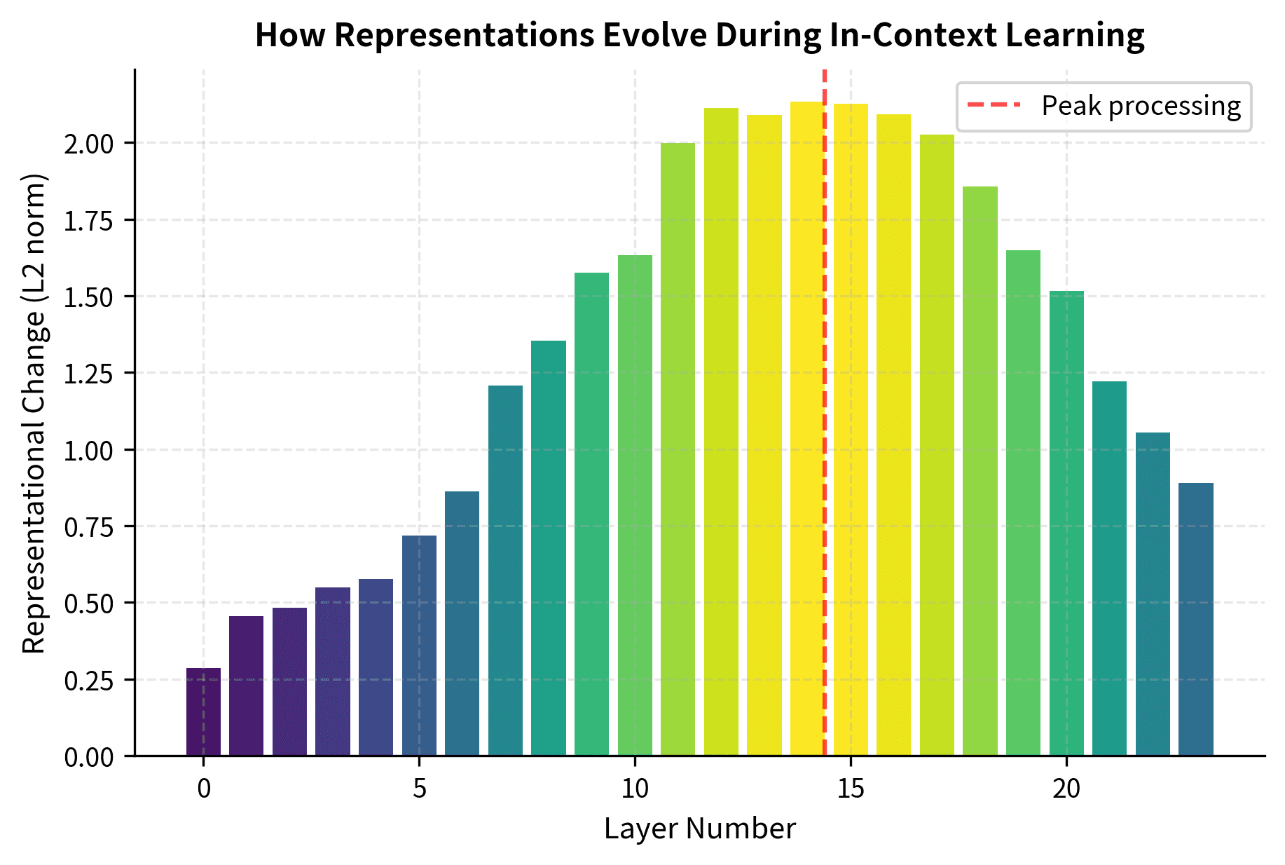
The analysis reveals that middle-to-late layers show the largest representational changes during ICL, suggesting that task-relevant processing concentrates in these layers rather than being distributed uniformly. This aligns with research showing that different layers serve different functions. Early layers handle basic pattern recognition, middle layers perform task-specific processing, and late layers prepare the final output.
Limitations and Impact
In-context learning has transformed what language models can accomplish, but important constraints remain. This section examines both the practical limitations and the broader impact of ICL emergence.
Current Limitations
Despite the remarkable capabilities of in-context learning, several significant limitations constrain its practical utility.
Context length constraints remain a fundamental bottleneck. ICL performance generally improves with more demonstrations, but the fixed context window limits how many examples can be provided. The techniques we covered in Part XV for extending context length help, but even million-token contexts fall short of the thousands of training examples that fine-tuning can leverage. This limitation is particularly acute for complex tasks that require diverse examples to cover the problem space.
Reliability and consistency present ongoing challenges. ICL performance can vary dramatically based on seemingly minor details: the order of demonstrations, the specific phrasing of examples, or the choice of delimiters. This sensitivity makes ICL less predictable than fine-tuning, where performance is typically more stable. Production systems using ICL often require careful prompt engineering and validation, adding complexity that the simplicity of few-shot learning was meant to eliminate.
Task complexity boundaries define another limitation. While ICL excels at tasks that can be demonstrated through a few examples, it struggles with tasks requiring extended reasoning, deep domain expertise, or complex multi-step procedures. The next chapter on chain-of-thought emergence explores how some of these limitations can be partially addressed through structured prompting approaches.
Computational efficiency at inference is often overlooked. While ICL eliminates training costs, it increases inference costs. Every query must process the full prompt including all demonstrations, making each inference more expensive than querying a fine-tuned model. For high-volume applications, this trade-off can make fine-tuning more economical despite its upfront costs.
Key Parameters
The key parameters affecting ICL emergence and performance are:
- Model scale: Number of parameters, typically measured in billions. ICL emergence thresholds vary by task but generally require 1B+ parameters for basic tasks and 10B+ for complex reasoning.
- Context length: Maximum number of tokens the model can process. Longer contexts allow more demonstrations but increase computational cost.
- Number of demonstrations (k-shot): More examples generally improve performance up to context limits, with diminishing returns.
- Temperature: Controls output randomness during generation. Lower values (0.0-0.3) typically work better for ICL tasks requiring precise answers.
- Demonstration ordering: The sequence of examples can significantly affect performance, with more recent examples often having stronger influence.
Transformative Impact
The emergence of in-context learning has changed how we build AI systems. Before ICL, deploying a model for a new task required collecting labeled data, fine-tuning, validation, and deploying task-specific model weights. This process took days to weeks and required machine learning engineering expertise.
With ICL, task adaptation becomes a matter of prompt design. A domain expert without machine learning training can configure a model for their specific use case by providing good examples. This shift has expanded who can build AI-powered applications and how quickly they can be developed.
The emergence of ICL also raised profound questions about what language models actually learn during pre-training. If a model can solve novel tasks from demonstrations, what does this say about its understanding? The mechanistic hypotheses we explored suggest that these models may be learning something deeper than text statistics, perhaps something closer to general-purpose reasoning and adaptation algorithms.
Summary
In-context learning emergence represents a qualitative shift in what language models can do. The key insights from this chapter:
Emergence patterns: ICL ability appears suddenly as models cross scale thresholds, typically between 1-10 billion parameters for basic tasks and larger scales for complex reasoning. This emergence is task-dependent, with simpler capabilities appearing earlier than complex ones.
Scaling comparison: Fine-tuning provides consistent improvements at all scales, while ICL shows emergent behavior. At large scales, few-shot ICL can match fine-tuning with orders of magnitude fewer examples, representing a fundamental shift in how we adapt models to new tasks.
Mechanism hypotheses: Multiple frameworks explain ICL. These include induction heads that implement pattern matching, implicit gradient descent in the forward pass, and task recognition versus task learning perspectives. These mechanisms likely coexist and contribute to overall ICL ability.
Meta-learning framework: Pre-training can be viewed as an outer loop that creates a general-purpose learning algorithm. The model learns not just to predict text, but to recognize tasks and adapt its behavior accordingly. This perspective explains both why ICL works and why it requires scale.
The emergence of ICL has transformed language models from static text predictors into dynamic few-shot learners. In the next chapter, we'll explore another emergent capability that builds on ICL: chain-of-thought reasoning, where models learn to decompose complex problems into explicit reasoning steps.
Quiz
Ready to test your understanding? Take this quick quiz to reinforce what you've learned about in-context learning emergence.

Comments