

Explore whether LLM emergent capabilities are genuine phase transitions or measurement artifacts. Learn how discontinuous metrics create artificial emergence.

This article is part of the free-to-read Language AI Handbook
Choose your expertise level to adjust how many terms are explained. Beginners see more tooltips, experts see fewer to maintain reading flow. Hover over underlined terms for instant definitions.
Emergence vs Metrics
The previous chapters painted a striking picture of emergent capabilities: abilities that appear suddenly at specific scales and are absent in smaller models but present in larger ones. These discontinuous jumps seemed to suggest something profound about how large language models acquire new capabilities. But a critical question has emerged in recent research: are we observing genuine phase transitions in model capability, or artifacts of how we measure performance?
This distinction matters. If emergence is real, it suggests that scaling models will unlock entirely new capabilities in unpredictable ways. If emergence is primarily a measurement artifact, capabilities may develop more gradually than accuracy curves suggest, and we can better predict what larger models will achieve.
The answer, as we'll see, lies in understanding the mathematics of measurement itself.
The Measurement Problem
When we evaluate language models on tasks, we face a fundamental choice: how do we convert continuous model outputs into discrete success/failure judgments? This choice has significant implications for how capabilities appear to develop.
Consider a multiple-choice question with four options. A model produces probability distributions over tokens, which we interpret as confidence in each answer choice. But benchmarks don't report these probabilities directly; they report whether the model got the answer right or wrong. This binary reduction throws away most of the information about what the model actually learned.
To see how severe this information loss is, consider a student taking a test. One student confidently writes the correct answer with complete certainty. Another student narrows down to two choices and makes an educated guess that happens to be right. A third student was 90% sure of the correct answer but second-guessed themselves at the last moment. Traditional grading treats all three identically: all three receive full marks. Yet clearly these students have different levels of understanding. The same information collapse occurs when we evaluate language models using binary accuracy metrics.
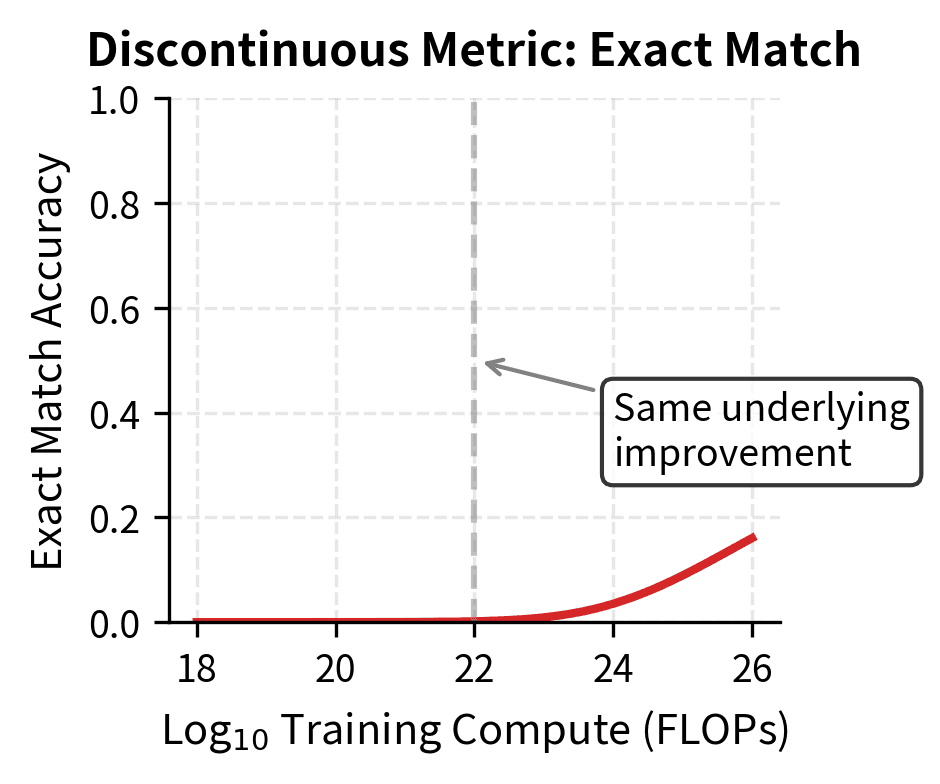
A discontinuous metric is one where the output (score) can jump abruptly based on small changes in the underlying model behavior. Accuracy and exact match are discontinuous. 99% confidence in the right answer scores the same as 100% confidence, while 49% confidence in a two-choice task scores zero.
The metrics we use for evaluation fall into two broad categories. Continuous metrics like cross-entropy loss, Brier score, or token-level log-probabilities can reveal gradual improvements. Discontinuous metrics like accuracy, exact match, or pass@1 collapse this information into binary outcomes.
To understand the difference concretely: if a model improves its confidence in the correct answer from 30% to 49%, a continuous metric like Brier score captures this substantial improvement, while accuracy still reports zero, since the model was "wrong" both times. The model has learned something valuable, becoming nearly twice as confident in the correct answer, yet our measurement instrument is blind to this progress.
Most emergence papers relied on discontinuous metrics. The sudden appearance of capabilities they documented may tell us more about the metrics than about the models.
Threshold Effects in Accuracy Metrics
To understand why discontinuous metrics create apparent emergence, we examine the mathematics of threshold effects. The core insight is that when we demand perfect sequential correctness, we transform what might be gradual improvement into an all-or-nothing proposition.
Consider a task where a model must generate an exact string like "The answer is 42." The model produces this string autoregressively, with some probability of generating the correct token at position given all previous tokens were generated correctly. Each token represents a checkpoint that the model must pass. Failing at any point means failing entirely.
The probability of generating the entire correct sequence is:
where:
- : the probability of generating the entire target string correctly
- : the probability of generating the -th correct token, given all previous tokens were correct
- : the total number of tokens in the target sequence
- : the product operator over all tokens, applying the chain rule of probability for sequential generation, where each token's probability is conditioned on all previous tokens being correct
This formula shows that sequential correctness is fragile. Unlike addition, where errors might partially cancel, multiplying probabilities means every imperfect step compounds the risk of failure. A chain is only as strong as its weakest link, and here we're multiplying all the links together. Think of it like a relay race where each runner must complete their leg perfectly. One stumble anywhere and the entire team loses, regardless of how well everyone else performed.
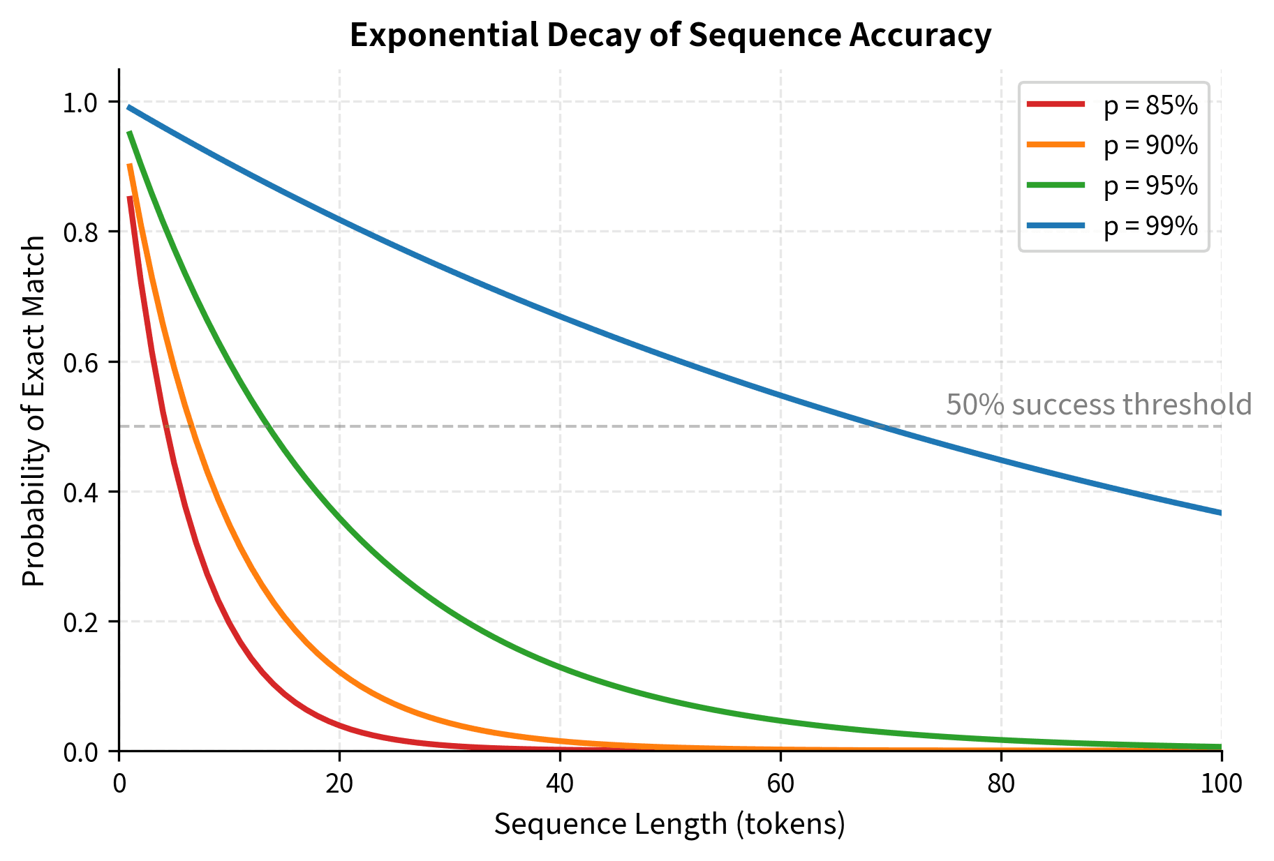
This multiplicative relationship is crucial: even small imperfections compound. If each token has a 95% chance of being correct, the probability of getting all tokens right shrinks rapidly as the sequence grows longer. What seems like excellent per-step performance (after all, 95% accuracy sounds impressive) leads to surprisingly poor overall outcomes when steps must chain together.
If we assume roughly uniform per-token accuracy across all tokens, this becomes:
This exponential relationship creates a threshold effect. The exponent acts as an amplifier, transforming modest changes in into dramatic changes in overall success probability. Suppose the model's per-token accuracy improves linearly with log compute from 80% to 99% over several orders of magnitude of scaling. For a 10-token answer:
| Per-token accuracy | Sequence accuracy |
|---|---|
| 80% | 10.7% |
| 85% | 19.7% |
| 90% | 34.9% |
| 95% | 59.9% |
| 99% | 90.4% |
The per-token accuracy improved smoothly from 80% to 99%, but sequence accuracy appears to "emerge" around the 95% per-token threshold. A model with 80% per-token accuracy looks like it has nearly zero capability on this task, but it's actually quite close to succeeding. This table shows a clear asymmetry: the jump from 95% to 99% per-token accuracy (a mere 4 percentage points) produces roughly the same sequence accuracy improvement as the entire journey from 80% to 95% (15 percentage points). The mathematics of multiplication creates this hockey-stick pattern automatically.

The heatmap reveals the "emergence zone" where sequence accuracy transitions rapidly from near-zero (red) to high performance (green). Notice how this transition zone shifts rightward for longer sequences. A 50-token task requires over 95% per-token accuracy to achieve even 50% sequence accuracy, while a 10-token task reaches the same performance at around 93% per-token accuracy.
The Amplification Problem
Longer sequences amplify this effect dramatically, turning modest measurement issues into severe distortions of apparent capability. The mathematical relationship between sequence length and success probability follows an inexorable exponential decay. For a 50-token sequence:
where:
- : the per-token accuracy (95% chance of getting each token correct)
- : the number of tokens in the target sequence
- : the result of multiplying 0.95 by itself 50 times
- : approximately 7.7% probability of generating the entire sequence correctly
To see why this happens, consider that means multiplying 0.95 by itself 50 times. Each multiplication slightly shrinks the result: , then , and so on. After 50 such multiplications, even starting from 95% per step, the cumulative probability has decayed to under 8%. This decay is relentless and mechanical. No amount of hoping or clever prompting can overcome the fundamental mathematics of multiplied probabilities.
Even a 95% per-token model achieves less than 8% exact match on a 50-token sequence. This model has substantial capability, but the exact match metric makes it appear completely incompetent. Consider a surgeon who performs each step of a 50-step procedure with 95% success. We would consider them highly skilled. Yet our evaluation framework would label their overall performance as a failure more than 92% of the time.
The relationship between per-token probability and sequence accuracy follows the exponential formula , where small changes in produce dramatic changes in for large . This mathematical structure is not a bug in our analysis; it is an accurate description of how exact-match evaluation works. The question is whether this evaluation accurately reflects the capability we care about, or whether it creates artificial cliffs that obscure genuine progress.
Notice how longer sequences push the "emergence threshold" higher. A task requiring 50-token outputs won't show above-chance accuracy until per-token probability exceeds roughly 97%. This creates the illusion that long-form generation capabilities emerge suddenly at large scales. The capability didn't emerge suddenly. Our measurement tool simply wasn't sensitive enough to detect the gradual improvement happening underneath.
Visualizing Smooth Capability with Discontinuous Metrics
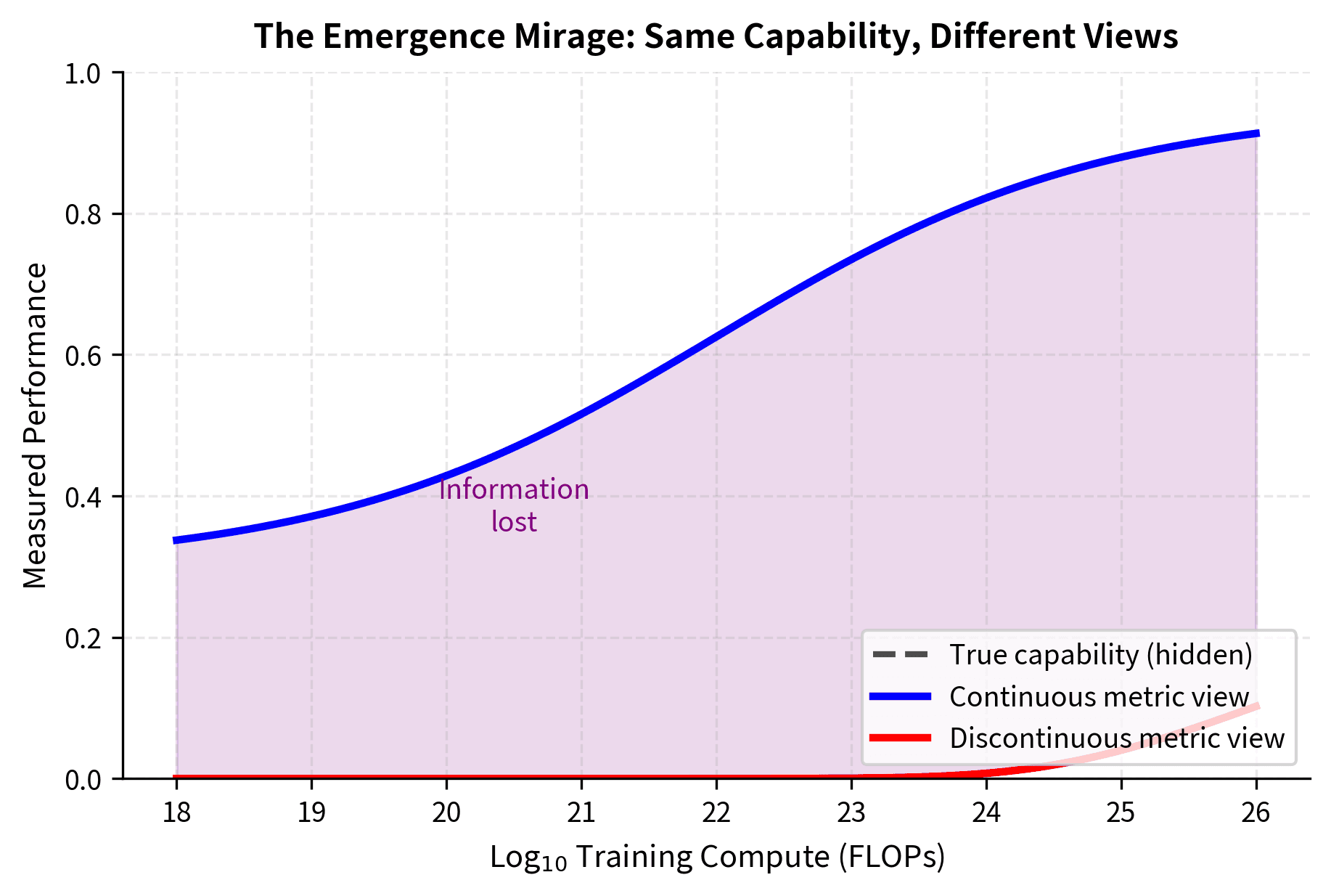
Let's create a simulation that demonstrates how smooth underlying improvements can appear as emergent transitions when measured with accuracy. This visualization will make the abstract mathematics concrete by showing exactly how the same underlying capability trajectory produces different apparent patterns depending on our choice of metric.
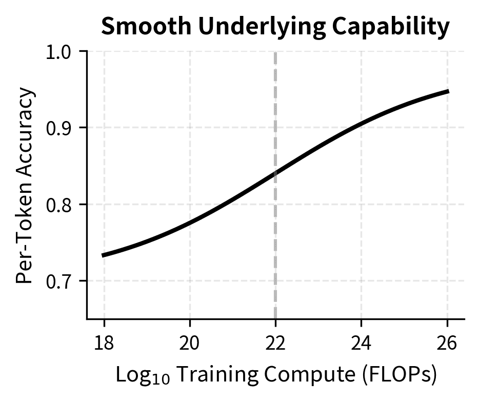
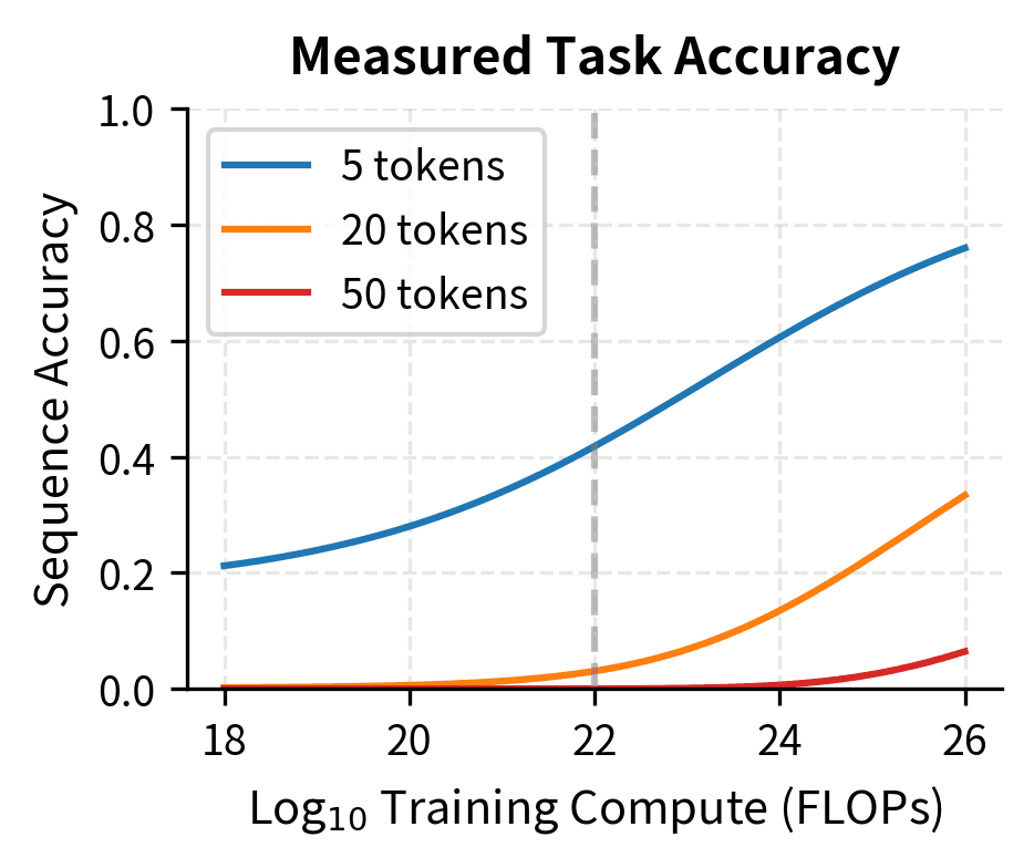
The left panel shows smooth, gradual improvement in the model's underlying capability. The right panel shows how this same improvement appears when measured by accuracy on sequences of different lengths. The 50-token task appears to "emerge" suddenly around FLOPs, while the 5-token task shows more gradual improvement. Yet the underlying capability change is identical. This visualization shows the core argument: emergence can be an optical illusion created by our measurement choices, not a fundamental property of how capabilities develop.
Multiple-Choice Tasks and Effective Answer Length
The same mathematics applies to multiple-choice questions, though the mechanism is slightly different. For a four-choice question, random performance is 25%. If the model must distinguish between answers that differ in the first few tokens, effective "sequence length" is short, and improvements appear more gradual.
However, many benchmark questions require understanding long contexts or performing multi-step reasoning before selecting an answer. The model's internal representations must correctly process many tokens to arrive at the right answer, even if the output is a single letter. This introduces a subtlety that the simple sequence-length formula does not capture directly, though the underlying multiplicative probability dynamics still apply. The difficulty of a task depends not just on how many output tokens we demand, but on how many internal computational steps the model must execute correctly.
The effective reasoning length of a task is the number of internal computational steps required to solve it correctly, regardless of output length. A math word problem answered with a single letter may require dozens of correct reasoning steps internally, making it effectively a long-sequence task.
This explains why complex reasoning tasks like those in BIG-Bench show more pronounced emergence than simple classification tasks: they have longer effective reasoning lengths, which amplifies the threshold effect. A task requiring the model to parse a complex sentence, identify relevant entities, retrieve world knowledge, apply logical rules, and synthesize a conclusion may involve the equivalent of a 30 or 40 "step" reasoning chain internally. Even if the final output is just "A" or "B", the threshold mathematics of multiplicative probabilities still applies to those internal steps, creating the same artificial emergence patterns we observe in long-form generation tasks.
Alternative Metrics Reveal Gradual Improvement
If emergence is a metric artifact, using continuous metrics should reveal the underlying gradual improvement. This is exactly what researchers have found. The key insight is that continuous metrics preserve information about model confidence that binary metrics discard, allowing us to observe the steady accumulation of capability that accuracy curves hide.
Brier Score and Probability Calibration
The Brier score measures the mean squared error between predicted probabilities and actual outcomes. It was originally developed for weather forecasting, where simply predicting "rain" or "no rain" throws away valuable information about confidence levels. A forecast of 90% chance of rain is more useful than a forecast of 51% chance of rain, even though both might lead to the same recommendation: carry an umbrella.
where:
- : the Brier score, measuring calibration quality (lower is better)
- : the total number of predictions being evaluated
- : the model's predicted probability for example (a value between 0 and 1, representing confidence in the positive class)
- : the actual outcome for example (1 if the positive class occurred, 0 otherwise)
- : the squared error for each prediction, penalizing confident wrong predictions heavily
- : the average over all predictions
The squaring is crucial: it penalizes large errors much more than small ones. A prediction of 0.9 for an event that does not happen () incurs error , while a prediction of 0.6 for the same outcome incurs only . This encourages the model to be conservative rather than overconfident. The quadratic penalty means that being confidently wrong is much worse than being uncertain, a property that aligns with our intuitions about what good predictions should look like.
The Brier score ranges from 0 (perfect predictions) to 1 (maximally wrong). A score of 0 would require perfect calibration: every event the model predicts with 70% confidence should occur 70% of the time, every event predicted with 30% confidence should occur 30% of the time, and so on. Unlike accuracy, which only cares whether , Brier score rewards improvements in probability even when they don't change the final prediction. A model moving from 40% to 49% confidence on a correct answer improves its Brier score despite both predictions being "wrong" by the accuracy metric. Unlike accuracy, Brier score rewards probability improvements even when they don't cross the decision threshold.
This property makes Brier score useful for tracking capability development. When a model improves from 30% to 45% confidence in correct answers, it has learned something meaningful about the task. Accuracy is blind to this progress, but Brier score captures it. The model is becoming more reliable even before it crosses the threshold into "correct" territory.

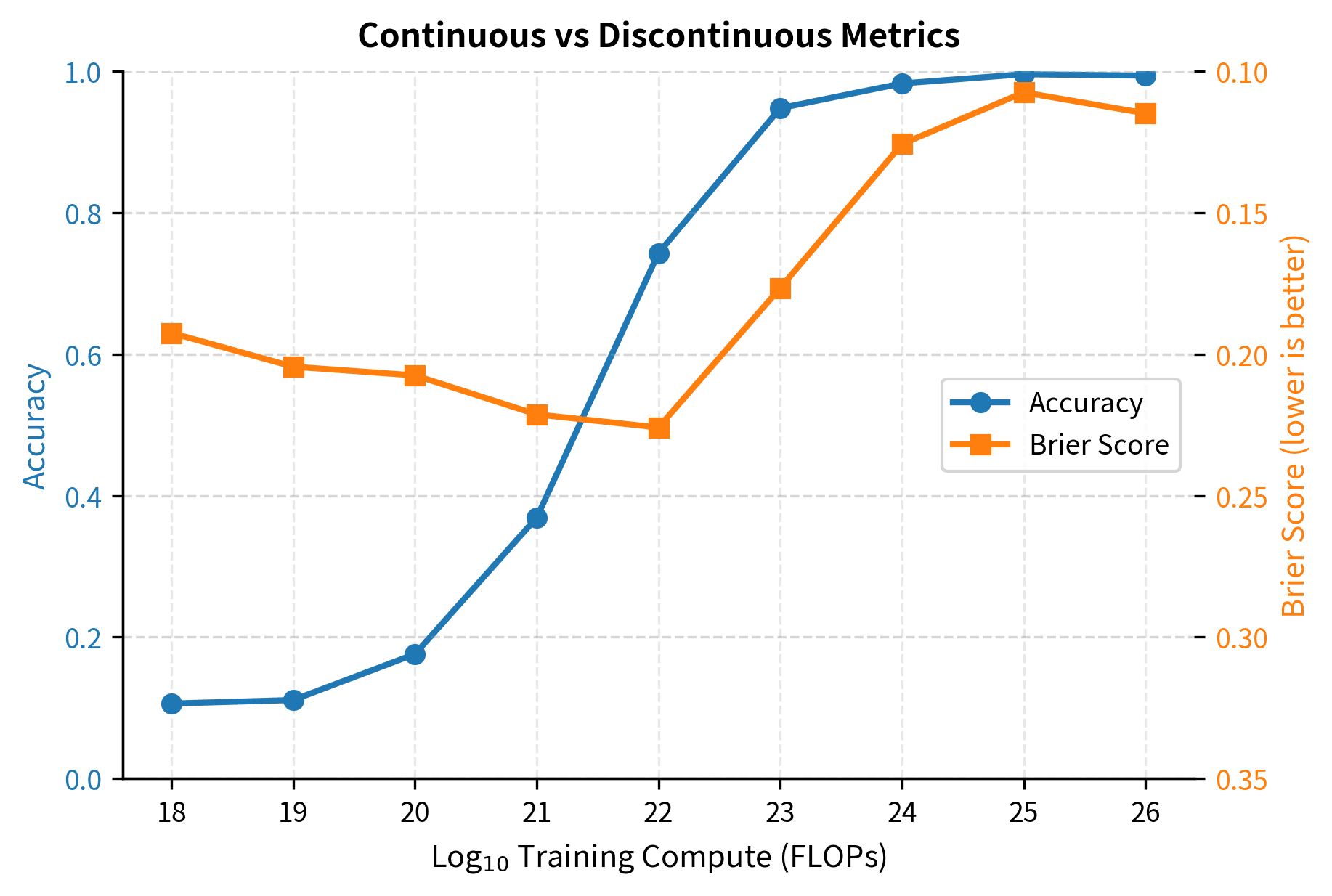
The Brier score improves smoothly across all scales, revealing the gradual capability development that accuracy obscures. While accuracy jumps from near-random to near-perfect performance, the Brier score shows steady, predictable improvement throughout. This is the same model, learning in the same way. Only our measurement lens has changed. The Brier score tells a story of continuous progress, while accuracy tells a story of sudden breakthrough. One of these stories is an artifact of the metric; the other reflects the underlying reality.
Token-Level Log-Probabilities
The most direct continuous metric is the average log-probability assigned to correct tokens. As we covered in our discussion of perplexity in Part II, this measures how surprised the model is by the correct answer. A model that assigns high probability to correct tokens is less surprised when it sees them, indicating it has learned something about the structure of correct responses.
For a correct output sequence , the average log-probability is:
where:
- : the average log-probability score, also known as the negative of per-token cross-entropy loss (higher/less negative indicates better predictions, with 0 being the theoretical maximum for perfect confidence)
- : the number of tokens in the correct output sequence
- : the -th token in the correct output sequence
- : all tokens preceding position (the context so far)
- : the input prompt or question
- : the model's predicted probability for token given the input and all previous correct tokens
- : the natural logarithm, which converts probabilities (0 to 1) to negative numbers (higher/less negative = more confident)
- : the average over all tokens in the sequence
The logarithm serves a specific purpose here: it converts multiplicative relationships into additive ones. Recall that sequence probability is the product of token probabilities: . Taking logs transforms this into a sum: . This makes the metric interpretable as an average per-token score rather than a product that shrinks toward zero for long sequences. By working in log space, we avoid the amplification problem that plagues exact-match metrics. Long sequences don't artificially suppress the measured capability.
This metric captures how "surprised" the model is by the correct answer. A model assigning 90% probability to each correct token will have a higher (less negative) average log-probability than one assigning 60%, even if both models ultimately generate the correct sequence.
To make this concrete: while . The 90%-confident model scores nearly 5 times better per token on this metric, capturing the substantial difference in capability that accuracy would miss if both models cross the decision threshold. This 5x difference in scores reflects a genuine difference in the models' internal states. One model has learned something meaningful about what makes answers correct, while the other is still somewhat uncertain. The average log-probability preserves this information rather than discarding it.
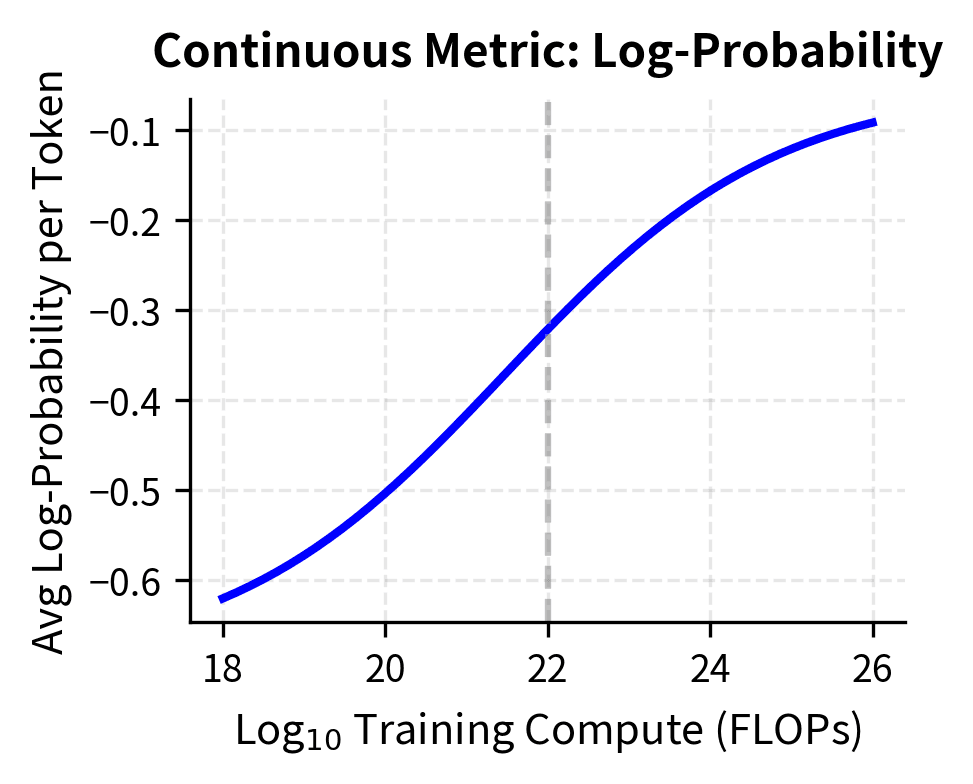
Studies examining emergence have found that this metric improves log-linearly with compute even for tasks where accuracy shows sharp transitions. The model's uncertainty about the correct answer decreases gradually; it's only the binary accuracy measurement that creates the appearance of sudden capability.
Re-examining Emergence Claims
In 2023, researchers at Stanford and Anthropic published a provocative paper titled "Are Emergent Abilities of Large Language Models a Mirage?" They systematically tested whether apparent emergence could be explained by metric choice alone.
The Experimental Approach
The researchers took tasks previously claimed to show emergence and re-evaluated models using continuous metrics. They found that for nearly all tasks examined:
- Accuracy showed sharp transitions consistent with prior emergence claims
- Continuous metrics showed smooth, predictable improvement across all scales
- The transition point was predictable from the metric and task structure
This pattern held across arithmetic, translation, word unscrambling, and other tasks that had been cited as evidence for emergent capabilities.
A Key Distinction
The mirage paper made an important distinction between two types of emergence:
Metric-induced emergence occurs when smooth underlying improvements appear discontinuous due to threshold effects in measurement. This is not truly "emergent" in any meaningful sense; the capability develops gradually and predictably.
True emergence would involve genuinely discontinuous changes in underlying capability: qualitative changes in how the model processes information that couldn't be predicted from smaller-scale behavior.
The paper argued that most documented cases of emergence are metric-induced, not true emergence.
When Might True Emergence Occur?
The metric critique doesn't eliminate the possibility of true emergence. Several mechanisms could produce genuine discontinuities.
Representational Phase Transitions
Neural networks may undergo qualitative changes in internal representations at certain scales. For example, a model might transition from storing specific facts to learning generalizable rules. Such transitions could produce genuine capability discontinuities.
Circuit Formation
As we discussed in our chapter on in-context learning emergence, some capabilities may require specific computational circuits that only form reliably at sufficient scale. The grokking phenomenon, which we'll explore in an upcoming chapter, shows that models can suddenly shift from memorization to generalization after extended training.
Compositional Generalization
Some capabilities require combining multiple subskills. If each sub-skill develops gradually but the combined capability requires all components simultaneously, the composite capability could emerge suddenly even with smooth sub-skill development. This mechanism differs fundamentally from metric-induced emergence. The discontinuity arises from the logical structure of the task itself, not from how we measure performance.
To understand this mechanism, consider learning to drive a car. Each individual skill (steering, braking, checking mirrors, reading traffic signs) can be practiced and improved gradually. But safely navigating an intersection requires all of these skills operating together correctly. A driver who excels at steering but forgets to check mirrors will fail the composite task. Similarly, one who reads signs but brakes too late will also fail. The intersection-navigation capability might "emerge" suddenly once all component skills exceed their required thresholds, even though no individual skill shows a phase transition.
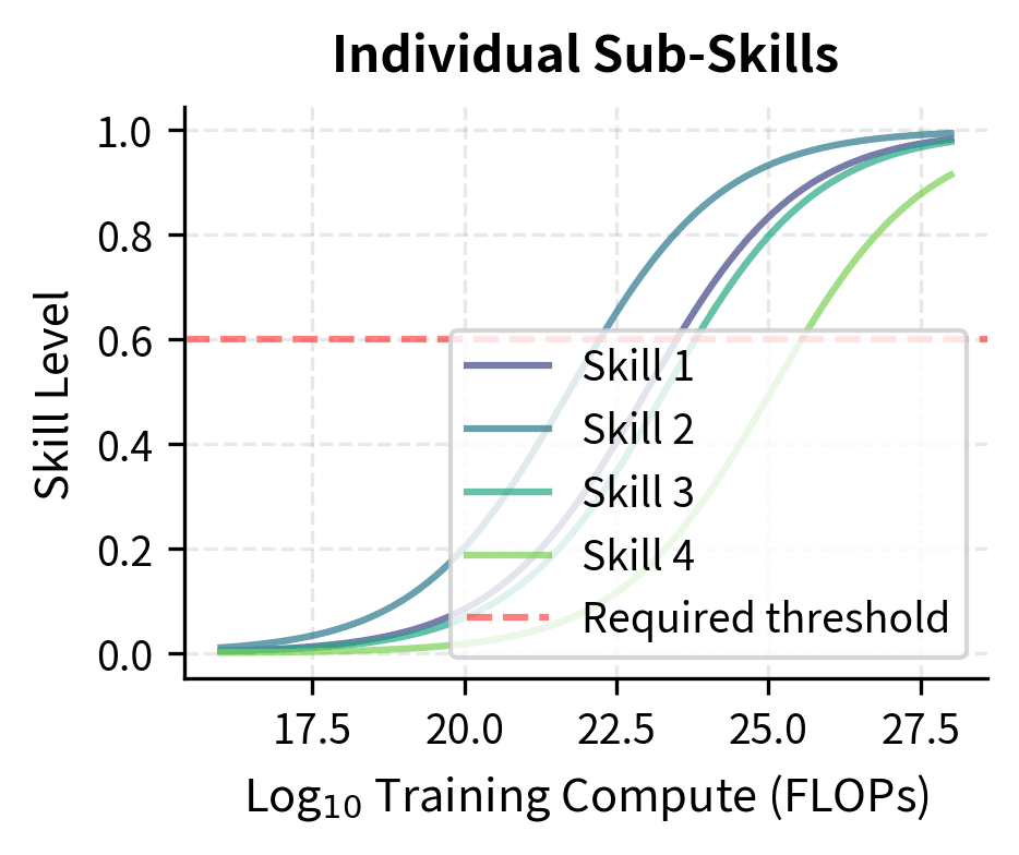
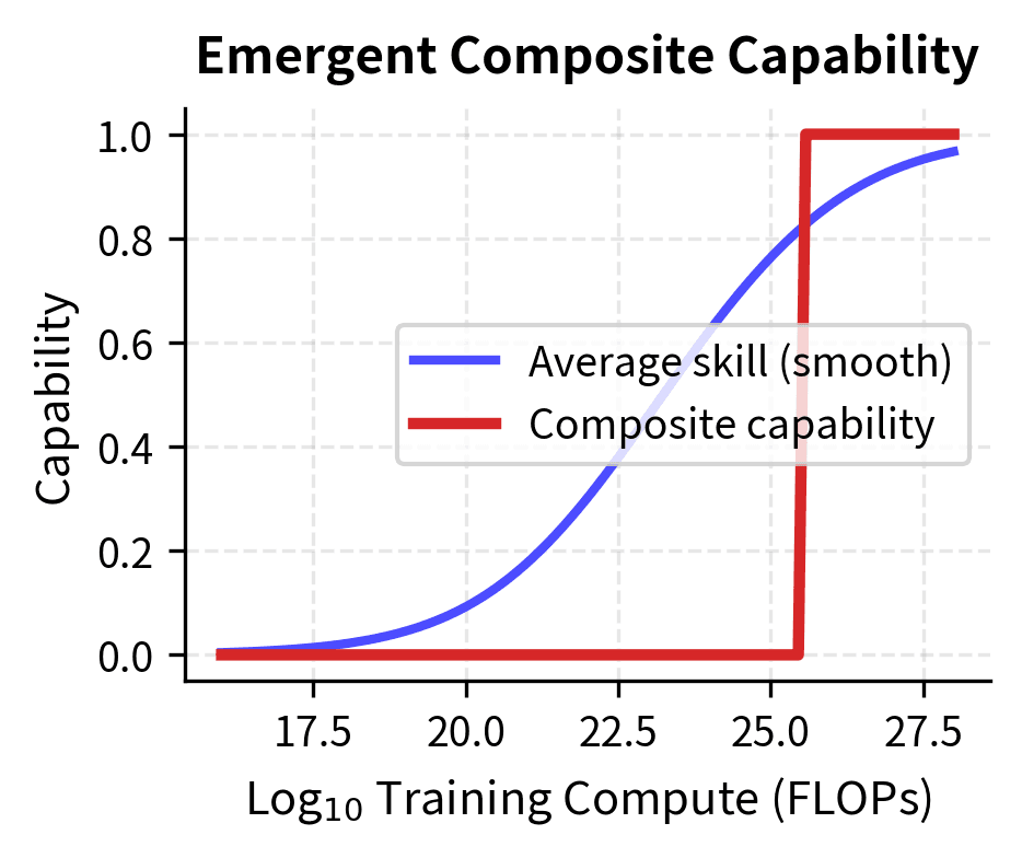
This type of compositional emergence is more subtle than metric-induced emergence. The individual skills develop smoothly, but the task requiring all skills shows a sharp transition. This could represent true emergence, or it could be another form of measurement artifact depending on how we define "capability." The key distinction is that compositional emergence reflects something real about task structure. Some tasks genuinely require multiple competencies to work together, rather than being purely an artifact of how we measure success.
Practical Implications for Evaluation
Understanding the distinction between metric-induced and true emergence affects how we evaluate and study language models.
Recommendations for Researchers
When studying capability development across scales, several practices can help distinguish metric artifacts from genuine phenomena:
-
Report multiple metrics. Always include at least one continuous metric alongside accuracy. Log-probability on correct tokens, Brier score, or calibration curves reveal whether underlying capability is improving.
-
Analyze per-token probabilities. For generation tasks, examine probability trajectories token-by-token rather than only sequence-level success.
-
Consider task decomposition. If a task can be broken into sub-tasks, measure performance on components separately to identify which, if any, show genuine discontinuities.
-
Control for effective sequence length. Tasks with longer required outputs or reasoning chains will show sharper transitions mechanically. Compare tasks of similar effective length when claiming differential emergence.
-
Test metric predictions. If emergence is metric-induced, changing the metric should eliminate the discontinuity. Test this explicitly.
Implications for Capability Prediction
The metric perspective helps with capability prediction. If capabilities develop smoothly, we can extrapolate performance to larger scales more reliably. The Chinchilla scaling laws we studied in Part XXI become more applicable. Rather than expecting unpredictable capability jumps, we can forecast how much compute is needed for specific capability levels.
However, this optimistic view assumes metric-induced emergence explains most cases. If some capabilities do emerge genuinely, perhaps through circuit formation or representational phase transitions, prediction remains challenging for those specific abilities.
Limitations and Ongoing Debates
The metric-induced emergence hypothesis explains many cases, but it's not universally accepted, and important questions remain.
One limitation is that the analysis focuses on task-level accuracy versus token-level probability. Some researchers argue this misses the possibility of emergence in internal representations. A model might develop new computational circuits or representational structures discontinuously, even if this manifests as smooth token-probability improvements. Studying internal representations directly, through probing or mechanistic interpretability techniques, could reveal forms of emergence invisible to behavioral metrics.
Additionally, the mirage paper primarily examined relatively simple tasks. More complex capabilities, like multi-step reasoning, theory of mind, or creative problem-solving, might behave differently. These capabilities may require qualitative changes in processing that truly emerge rather than develop gradually. The chain-of-thought reasoning we explored in the previous chapter could involve genuine circuit formation that enables new types of computation.
There is also debate about whether this distinction matters practically. If a capability appears to emerge regardless of the underlying mechanism, users experience a discontinuous jump in model utility. From an engineering perspective, metric-induced emergence may be indistinguishable from true emergence in its practical effects.
Finally, the metric perspective does not explain why different capabilities emerge at different scales. Even if all emergence is metric-induced, understanding which capabilities require more scale and why remains an important research question.
Summary
This chapter examined the relationship between how we measure capabilities and how capabilities appear to develop. The key insights include:
-
Discontinuous metrics create apparent emergence. Accuracy and exact match metrics can make smooth underlying improvements appear as sudden capability jumps due to threshold effects.
-
Sequence length amplifies discontinuity. Tasks requiring longer outputs or more reasoning steps show sharper apparent transitions, even when per-token capability improves smoothly.
-
Continuous metrics reveal gradual improvement. Brier score, log-probabilities, and other continuous metrics typically show smooth, predictable scaling where accuracy shows sharp emergence.
-
Most documented emergence may be metric-induced. Research re-examining emergence claims found that continuous metrics eliminated apparent discontinuities for most tasks studied.
-
True emergence remains possible. Compositional requirements, circuit formation, and representational phase transitions could produce genuine capability discontinuities, though these are harder to document conclusively.
-
Evaluation practices should adapt. Researchers should report multiple metrics and analyze per-token probabilities to distinguish metric artifacts from genuine phenomena.
Key Parameters
The key parameters and concepts for understanding emergence metrics are:
- per_token_prob (p): The probability of generating each correct token. Small improvements in per-token probability can produce dramatic changes in sequence accuracy.
- sequence_length (n): The number of tokens in the target output. Longer sequences amplify threshold effects exponentially.
- Brier score: A continuous metric measuring mean squared error between predictions and outcomes. Unlike accuracy, it captures improvement even below decision thresholds.
- threshold: The decision boundary (typically 0.5) where predictions flip from negative to positive class. Accuracy only changes when probabilities cross this boundary.
The next chapter examines inverse scaling, a counterintuitive phenomenon where larger models sometimes perform worse on specific tasks. This challenges even the basic assumption that more scale produces more capability.
Quiz
Ready to test your understanding? Take this quick quiz to reinforce what you've learned about emergence and measurement artifacts.

Comments