

Learn how AdaLoRA dynamically allocates rank budgets across weight matrices using SVD parameterization and importance scoring for efficient model adaptation.

This article is part of the free-to-read Language AI Handbook
Choose your expertise level to adjust how many terms are explained. Beginners see more tooltips, experts see fewer to maintain reading flow. Hover over underlined terms for instant definitions.
AdaLoRA
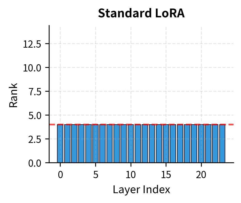
Standard LoRA applies the same rank to every adapted weight matrix in a model. A query projection receives the same adaptation capacity as a value projection, and attention layers receive the same as feed-forward layers. This uniform allocation ignores a fundamental insight: different weight matrices contribute differently to task performance. Some weight matrices require substantial adaptation while others barely need any.
AdaLoRA (Adaptive Low-Rank Adaptation) addresses this limitation by dynamically allocating rank budgets across weight matrices during training. Rather than fixing ranks beforehand, AdaLoRA starts with a high rank for all matrices, measures which components contribute most to performance, and progressively prunes the less important ones. The result is an intelligent distribution of adaptation capacity: more rank where it matters, less where it doesn't, all while staying within a fixed parameter budget.
This chapter covers the technical foundations of AdaLoRA: how its SVD-based parameterization enables fine-grained pruning, how importance scores identify which components to keep, and how the training procedure orchestrates dynamic rank allocation. Building on the LoRA fundamentals from previous chapters, you'll see how a simple change in parameterization unlocks substantially more efficient adaptation.
SVD-Based Parameterization
Recall from our LoRA discussion that standard LoRA represents weight updates as:
where:
- : the downstream projection matrix of dimension
- : the upstream projection matrix of dimension
This product produces a rank- matrix, but the individual columns of and rows of are entangled: you cannot remove one column-row pair without affecting the entire product's behavior unpredictably. To understand why this entanglement poses a problem, consider what happens when you try to prune a component. If you remove the third column of and the third row of , the remaining columns and rows still interact in complex ways during the matrix multiplication. The contribution of each column-row pair depends on all the others, making it impossible to cleanly isolate and evaluate individual components.
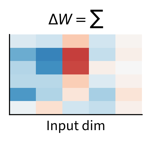
AdaLoRA adopts an SVD-inspired parameterization that decouples these components, providing a clean solution to the entanglement problem:
where:
- contains orthonormal columns (left singular vectors)
- is a diagonal matrix of singular values
- contains orthonormal rows (right singular vectors)
This parameterization resembles a truncated SVD, though , , and are learned rather than computed from an existing matrix. The key advantage is separability: each triplet contributes independently to the weight update. This independence arises from the orthonormality constraints on and . When the columns of are orthogonal to each other, and the rows of are orthogonal to each other, each singular value triplet occupies its own distinct "direction" in the weight update space. Removing one triplet leaves the others completely unchanged, enabling precise surgical pruning of adaptation components.
Singular Value Decomposition expresses any matrix as , where and have orthonormal columns and is diagonal with non-negative singular values. AdaLoRA uses a similar structure but learns the components directly, allowing negative singular values and soft orthonormality.
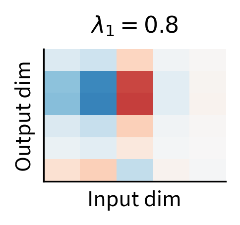
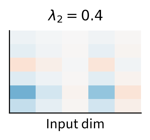
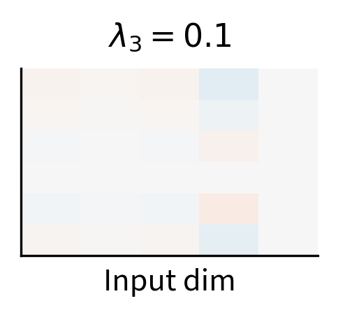
The contribution of the -th component to the weight update is simply:
where:
- : the contribution of the -th singular value triplet to the weight update
- : the -th singular value scalar
- : the -th column of the left singular matrix
- : the -th row of the right singular matrix
This is a rank-1 matrix scaled by . The outer product creates a matrix where each entry is the product of corresponding elements from the column vector and row vector. Multiplying by the scalar scales this entire rank-1 contribution. This formulation makes pruning straightforward: setting completely removes this component from the update without affecting the others. This property is what makes importance-based pruning tractable: we can evaluate and remove individual components rather than having to analyze the entire matrix. Each component can be assessed on its own merits, kept or discarded based on its contribution to task performance.
Orthonormality Constraints
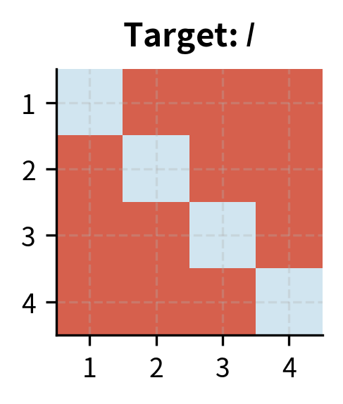
For the decomposition to maintain its SVD-like properties, and should have orthonormal columns and rows respectively. Orthonormality means two things simultaneously: each column of should have unit length (normality), and different columns should be perpendicular to each other (orthogonality). The same applies to the rows of . These constraints ensure that the singular value triplets remain independent and that the singular values directly represent the magnitude of each component's contribution.
During training, AdaLoRA enforces this approximately through a regularization term:
where:
- : the regularization term added to the loss
- : the Frobenius norm
- : the identity matrix
- : the deviation from column orthonormality for
- : the deviation from row orthonormality for
The first term penalizes deviation from orthonormality in 's columns. To see why this works, consider what represents. The entry of this matrix equals the dot product of the -th and -th columns of . If , then , meaning columns are unit-length (diagonal entries equal 1) and mutually orthogonal (off-diagonal entries equal 0). The second term enforces the same for 's rows, where captures the dot products between different rows.
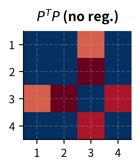
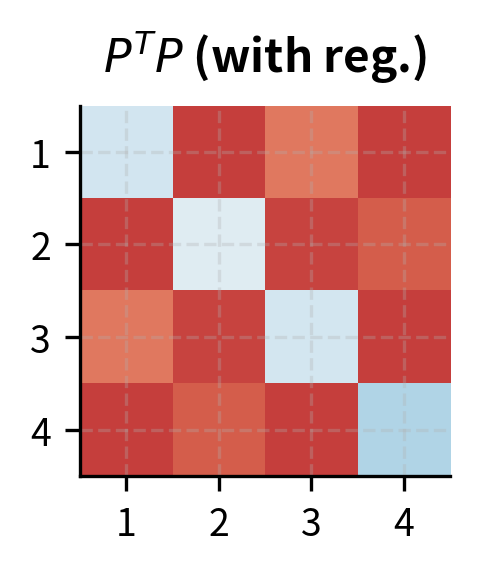
This soft constraint offers a practical trade-off between mathematical purity and computational efficiency. Hard orthonormality (using Gram-Schmidt or similar projection methods) would require expensive projections after each gradient step, fundamentally changing the optimization landscape. The regularization approach allows the optimizer to handle orthonormality as just another objective, balancing it against the task loss naturally. The optimizer can temporarily violate orthonormality if doing so helps reduce the task loss, then gradually restore the constraint as training progresses. This flexibility often leads to better final solutions than rigid enforcement would allow.
Importance Scoring
The heart of AdaLoRA is deciding which singular value triplets to keep and which to prune. This requires an importance score that reflects each component's contribution to model performance. The challenge lies in defining "importance" in a way that captures both current contribution and future potential. A component might currently have a small effect but be rapidly learning something crucial, or it might have a large effect but be stable and potentially redundant.
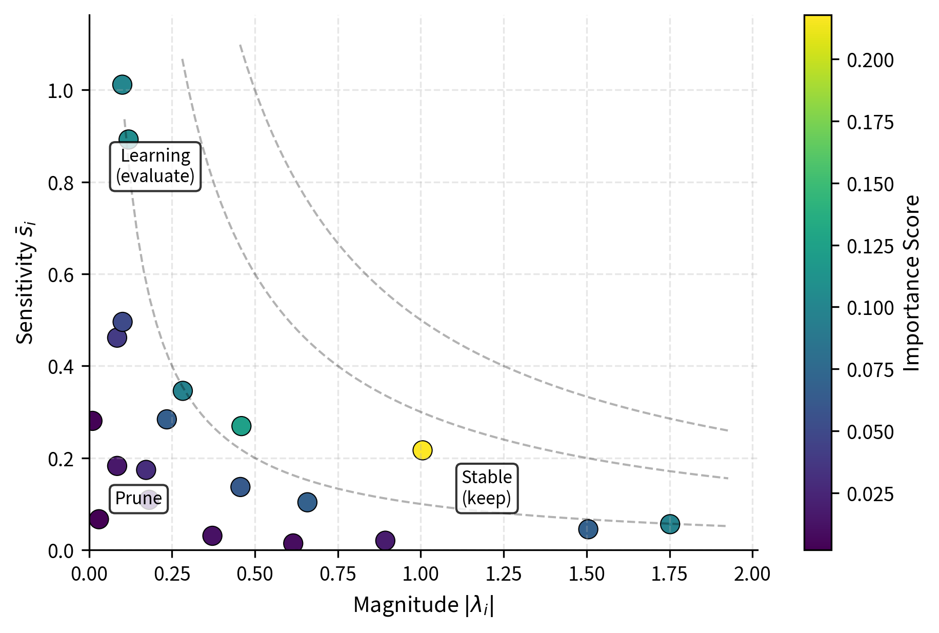
Magnitude and Sensitivity
A naive approach would rank components by : larger singular values contribute more to the weight update's magnitude. This makes intuitive sense because the singular value directly scales the rank-1 contribution to the weight update. However, magnitude alone misses crucial information about gradient flow. A large singular value with near-zero gradients is stable and well-fitted, meaning it has found its optimal value and further changes would not improve performance. A smaller singular value with large gradients is actively being updated and may be critical for learning, representing a component that the optimization process is still working to refine.
AdaLoRA combines both signals into an importance score:
where:
- : the importance score for the -th component
- : the sensitivity term derived from gradient information
- : the magnitude of the singular value
The sensitivity captures how much the loss would change if were perturbed. This combination balances two complementary views of importance. The magnitude term captures the current state: how much does this component actually contribute right now? The sensitivity term captures the dynamics: how actively is the optimization process adjusting this component? Together, they identify components that are both currently contributing and likely to continue contributing as training progresses.
Sensitivity Estimation
The sensitivity for singular value is computed as:
where:
- : the instantaneous sensitivity at step
- : the value of the singular value at step
- : the gradient of the loss with respect to the singular value
This formulation estimates the change in loss if the singular value were removed (set to zero). The intuition is straightforward: we want to know how much the loss would increase if we eliminated this component entirely. We can derive this using a first-order Taylor expansion:
This expansion approximates the change in loss as a linear function of the change in parameter value, with the gradient serving as the proportionality constant. If we prune the component, the change in the parameter is . Substituting this gives:
This quantity serves as a proxy for feature importance, often called "saliency" in pruning literature. Components with high saliency would cause large loss increases if removed, making them essential for model performance. Components with low saliency can be safely pruned with minimal impact on the loss.
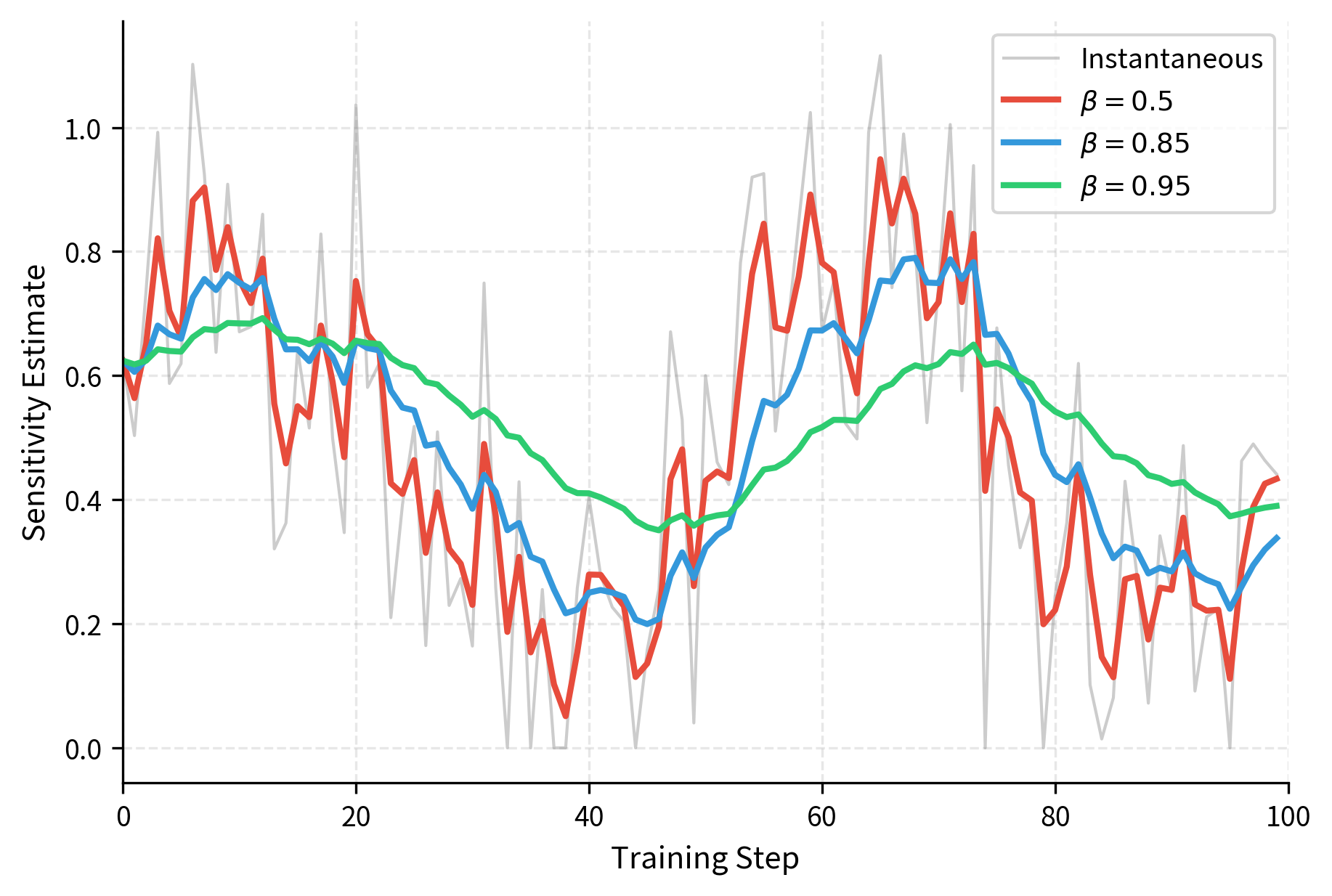
To reduce noise from stochastic gradients, AdaLoRA maintains an exponential moving average:
where:
- : the smoothed sensitivity estimate at step
- : the smoothing parameter (typically around 0.85)
- : the instantaneous sensitivity from the current step
This averaging stabilizes importance estimates across mini-batches, preventing premature pruning decisions based on noisy gradient samples. Because gradients computed on small mini-batches can vary substantially from step to step, a single noisy gradient could incorrectly suggest that an important component is unimportant, or vice versa. The exponential moving average smooths out this noise by giving weight to the entire history of gradient observations, with more recent observations weighted more heavily. The parameter controls the balance: higher values create smoother estimates but respond more slowly to genuine changes in importance.
Full Importance Formula
The complete importance score incorporates the orthonormal vectors as well:
where:
- : the final importance score
- : the Frobenius norm (length) of the -th column of
- : the Frobenius norm (length) of the -th row of
- : the output and input dimensions of the layer
The inclusion of the vector norms accounts for the fact that the orthonormality constraint is enforced softly rather than exactly. If the vectors have grown larger or smaller than unit length, this affects the actual magnitude of the contribution to the weight update. The normalization by and ensures scores are comparable across layers with different dimensions. Without this normalization, layers with larger dimensions would naturally have larger vector norms, potentially biasing the pruning toward keeping components in smaller layers regardless of their actual importance.
When the orthonormality constraint is well-satisfied, and , simplifying the score to approximately . This simplified form shows that the full formula simplifies to the combination of sensitivity and magnitude when the SVD structure is well-maintained.
Dynamic Rank Allocation
With importance scores in hand, AdaLoRA can allocate rank budgets across all weight matrices in the model. The process operates under a global budget constraint: the total number of singular value triplets across all adapted matrices must not exceed a target budget . This global perspective is essential because it allows the algorithm to make intelligent trade-offs, giving more capacity to layers that need it while reducing capacity for layers that can work with less.
Global Ranking
Rather than allocating ranks layer-by-layer, AdaLoRA performs global ranking across all singular values in all adapted weight matrices. If the model adapts weight matrices, each initialized with rank , there are total triplets. These are all ranked by their importance scores, and the top are retained. This creates a competition across the entire model: every singular value triplet must justify its existence relative to all others.
This global approach naturally handles heterogeneity across layers. If attention layers consistently show higher importance scores than feed-forward layers, they automatically receive higher ranks. No manual configuration is needed since the data determines the allocation. This is a significant advantage over approaches that require practitioners to manually specify different ranks for different layer types based on intuition or expensive hyperparameter searches. The algorithm discovers the optimal allocation through the natural process of training, adapting to the specific characteristics of the task and dataset.
Pruning Schedule
Pruning doesn't happen all at once. Removing many components simultaneously could destabilize training, and early importance estimates may not reflect true long-term importance. AdaLoRA follows a schedule that gradually reduces the total budget from the initial to the final target :
where:
- : the rank budget at training step
- : the final target budget
- : the initial total budget across all layers
- : the current training step
- : the warmup period steps
- : the total number of training steps
This cubic schedule starts with aggressive pruning (when many obvious candidates exist) and slows down as the budget approaches its target (when decisions become more consequential). The cubic function ensures that the rate of pruning decreases smoothly over time. Early in training, when the budget is far from the target, large numbers of components are pruned at each step. As training progresses and the budget approaches its target, fewer components are pruned, giving the algorithm more time to carefully evaluate the remaining candidates.
The warmup period is crucial. During warmup, no pruning occurs, allowing importance estimates to stabilize. Pruning too early risks removing components that are important but haven't yet accumulated sufficient gradient statistics. In the first few steps of training, gradient estimates are particularly noisy because the model is still adjusting to the new task. A component might appear unimportant simply because it hasn't received enough gradient signal to reveal its true importance. The warmup period ensures that every component has a fair chance to demonstrate its value before any pruning decisions are made.
Masking Mechanism
When a singular value triplet is pruned, AdaLoRA sets via a binary mask rather than removing the parameters entirely. This serves two purposes:
- Memory efficiency: Masking avoids dynamic memory reallocation during training
- Potential recovery: In some implementations, pruned components could theoretically be reactivated if their importance increases
The masking approach means the actual parameter count doesn't change during training since all triplets remain in memory. However, the effective rank (number of non-zero singular values) decreases according to the schedule. This distinction between nominal and effective parameters is important for understanding AdaLoRA's resource usage. Training requires memory for all initial parameters, but the final model's computational cost depends only on the effective parameters that survive pruning.
Training Procedure
The complete AdaLoRA training procedure integrates the elements described above into a coherent algorithm. Understanding how these pieces fit together illuminates why AdaLoRA works effectively and how its various components interact during optimization.
Initialization
Training begins by initializing the SVD-style decomposition for each adapted weight matrix:
- Initialize with random orthonormal columns (e.g., from QR decomposition of a random matrix)
- Initialize as zeros (same as LoRA's initialization strategy)
- Initialize with random orthonormal rows
- Set all importance score accumulators
The zero initialization of ensures the model starts from the pretrained weights, just as in standard LoRA. This initialization strategy is crucial because it means that at the start of training, . The adapted model begins identical to the pretrained model, and the adaptation components gradually grow from zero as training progresses. This prevents any sudden changes to the model's behavior at the start of fine-tuning.
Training Loop
Each training iteration proceeds as follows:
- Forward pass: Compute predictions using adapted weights
- Loss computation: Calculate task loss plus orthogonality regularization
- Backward pass: Compute gradients for , , and
- Update importance scores: Update exponential moving averages using current gradients
- Parameter update: Apply optimizer step to , , and
- Pruning (if scheduled): If past warmup and at a pruning step, mask lowest-importance singular values
The pruning step typically occurs every few hundred iterations rather than every step, reducing computational overhead and allowing importance estimates to update between pruning decisions. This periodic pruning also provides stability: rather than constantly adjusting the active set of components, the model has time to adapt to each pruning decision before the next one occurs.
Final Rank Distribution
After training completes, different weight matrices will have different effective ranks. A typical pattern shows:
- Query and value projections: Higher ranks, often retaining most of their initial budget
- Key projections: Moderate ranks
- Output projections: Variable, task-dependent
- Feed-forward layers: Often lower ranks, especially in deeper layers
This distribution emerges entirely from the data and task since AdaLoRA discovers it rather than requiring manual specification. The patterns often reveal interesting insights about which parts of the model are most important for the specific task being fine-tuned. Query and value projections tend to receive higher ranks because they directly influence what information the model attends to and how it combines attended information, both crucial for most downstream tasks.
Code Implementation
Let's implement AdaLoRA using the PEFT library, which provides a clean interface for this technique.
We'll configure AdaLoRA with its key hyperparameters. The most important are the initial rank and target rank, which define the budget reduction during training.
Let's examine the parameter structure that AdaLoRA creates.
The trainable parameter count reflects the initial rank across all adapted matrices. This count will effectively decrease during training as singular values are pruned (though the actual parameters remain, just zeroed out).
Inspecting SVD Components
Let's look at how AdaLoRA structures its parameters compared to standard LoRA.
Each AdaLoRA layer contains (called lora_A in PEFT), (called lora_E), and (called lora_B).
The final loss indicates the model has successfully adapted to the training data. The reduction in loss implies that the rank allocation strategy effectively optimized the parameters.
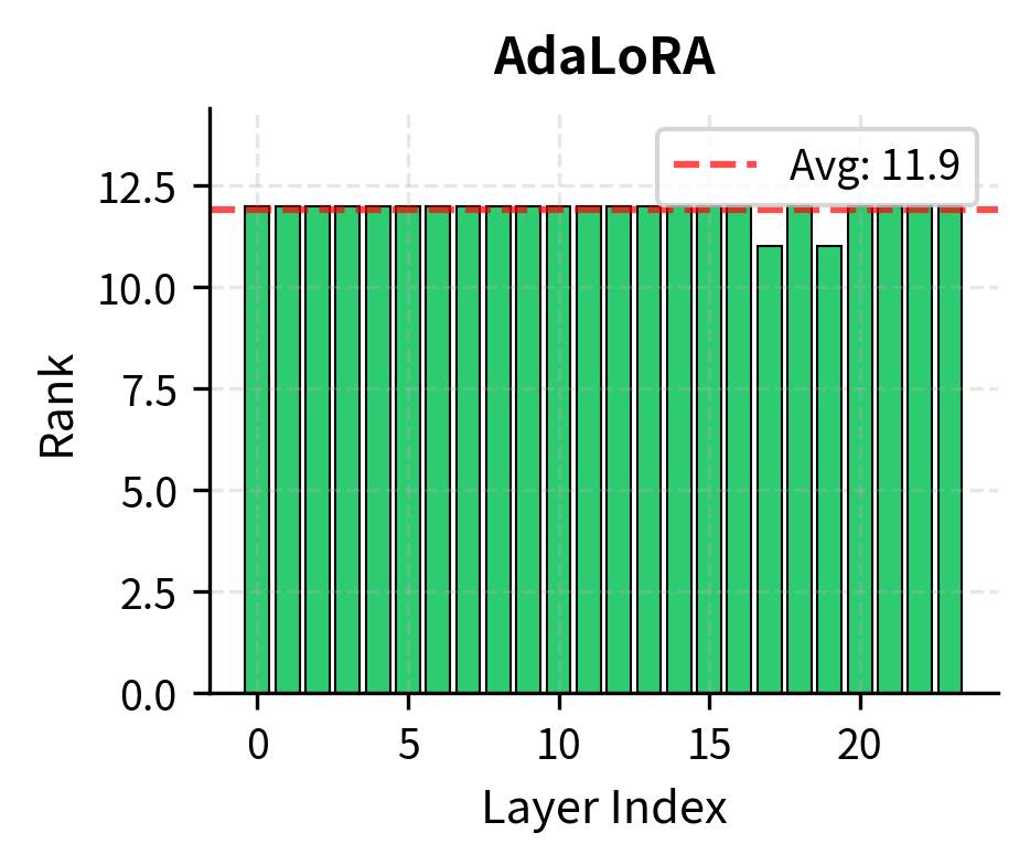
Examining Final Rank Distribution
After training, we can inspect how AdaLoRA distributed ranks across different layers.
The distribution reveals which layers AdaLoRA determined were most important for this task. Layers with higher retained ranks contribute more to the adaptation.
Visualizing Rank Evolution
The cubic pruning schedule is evident: aggressive rank reduction early in training (when many clearly unimportant components exist) followed by gentler pruning as the budget approaches its target.
Comparing with Standard LoRA
To appreciate AdaLoRA's benefits, let's compare the parameter efficiency at equivalent performance levels.
The parameter counts are similar, but AdaLoRA's adaptive allocation can achieve better performance by concentrating parameters where they matter most.
Key Parameters
The key parameters for AdaLoRA are:
- init_r: The initial rank allocated to all matrices before pruning begins.
- target_r: The final average rank to achieve across all adapted matrices.
- beta1/beta2: Smoothing factors for the exponential moving averages of gradient sensitivity and importance scores.
- orth_reg_weight: The strength of the regularization term that enforces orthonormality of singular vectors.
- total_step: The total number of training steps, used to calculate the pruning schedule.
Limitations and Impact
AdaLoRA introduced an important insight to parameter-efficient fine-tuning: not all weight matrices are equally important, and adaptive allocation can improve efficiency. However, the technique comes with trade-offs worth understanding.
The primary limitation is training overhead. AdaLoRA must maintain importance score accumulators for every singular value triplet, compute exponential moving averages at each step, and periodically evaluate global rankings for pruning decisions. The orthogonality regularization adds an additional loss term requiring its own gradient computation. In practice, this can increase training time by 20-30% compared to standard LoRA, though the final model is no more expensive at inference.
The SVD-style parameterization also introduces hyperparameter sensitivity. The orthogonality regularization weight must be balanced against the task loss: too weak and the decomposition loses its SVD-like properties, too strong and it interferes with learning. The pruning schedule parameters (warmup length, cubic decay rate) interact with learning rate schedules in complex ways. Getting these right often requires more tuning than standard LoRA's simpler setup.
Memory consumption during training is another consideration. While AdaLoRA can produce a smaller final model (in effective parameters), training starts with the full initial rank and stores importance statistics for all components. This can actually require more memory than training standard LoRA at the target rank, though less than training at the initial rank without pruning.
Despite these limitations, AdaLoRA demonstrated that rank allocation matters and can be learned rather than hand-tuned. This inspired subsequent work on dynamic adaptation methods. The technique performs particularly well when there's significant heterogeneity in how different layers contribute to a task, as often occurs in transfer learning scenarios where some pretrained representations align well with the target task while others need substantial modification.
The principles from AdaLoRA also influenced thinking about model compression more broadly. The importance-weighted pruning approach, combining magnitude with gradient sensitivity, has been adopted in other contexts beyond low-rank adaptation. We'll see related ideas appear when we examine other PEFT methods like IA³ and prefix tuning in upcoming chapters, each offering different trade-offs between adaptation expressivity and parameter efficiency.
Summary
AdaLoRA extends standard LoRA with adaptive rank allocation, addressing the limitation that uniform ranks across all weight matrices may not reflect their varying importance to task performance.
The key innovations are:
- SVD-based parameterization using with orthonormal and , enabling independent pruning of singular value triplets
- Importance scoring that combines parameter magnitude with gradient-based sensitivity, smoothed via exponential moving averages
- Global ranking across all adapted matrices, allowing automatic discovery of which layers need more adaptation capacity
- Cubic pruning schedule with warmup, aggressively removing unimportant components early while being conservative near the target budget
The training procedure integrates these elements: initialize at high rank, accumulate importance statistics during warmup, progressively prune to target budget, and maintain approximate orthonormality throughout. The result is an intelligent distribution of adaptation parameters that can outperform uniform-rank LoRA at equivalent parameter budgets.
While AdaLoRA's overhead makes it less suitable for quick experiments, its adaptive allocation is valuable for production deployments where squeezing maximum performance from a fixed parameter budget justifies additional training cost.
Quiz
Ready to test your understanding? Take this quick quiz to reinforce what you've learned about AdaLoRA and adaptive rank allocation.

Comments