

Learn to implement LoRA adapters in PyTorch from scratch. Build modules, inject into transformers, merge weights, and use HuggingFace PEFT for production.

This article is part of the free-to-read Language AI Handbook
Choose your expertise level to adjust how many terms are explained. Beginners see more tooltips, experts see fewer to maintain reading flow. Hover over underlined terms for instant definitions.
LoRA Implementation
Having explored the mathematical foundations of LoRA in the previous chapter, we now turn to the practical challenge of translating those equations into working code. The elegance of LoRA lies not just in its theoretical properties, but in how naturally it fits into existing neural network frameworks. A well-designed LoRA module should integrate seamlessly with pre-trained models, require minimal changes to training code, and support efficient inference through weight merging. This transition from theory to practice makes the concepts more concrete.
This chapter walks through the complete implementation journey, providing both the conceptual understanding and the working code you need to apply LoRA in your own projects. We start by designing a reusable LoRA module that encapsulates the low-rank decomposition, explaining each design decision along the way. From there, we build the machinery to inject LoRA into existing transformer layers, enabling you to adapt any compatible model with just a few lines of code. We then construct a training loop that updates only the adaptation parameters, demonstrating the memory efficiency that makes LoRA practical for limited hardware. The chapter proceeds to implement weight merging for deployment, showing how to eliminate runtime overhead when moving to production. Finally, we conclude with practical guidance on using HuggingFace's PEFT library, which provides production-ready implementations of these concepts and integrates with the broader transformers ecosystem.
LoRA Module Design
The core building block of any LoRA implementation is a module that wraps an existing linear layer and adds the low-rank adaptation path. This wrapper pattern is fundamental to LoRA's design philosophy: rather than modifying the original model architecture, we augment it with a parallel pathway that learns task-specific adjustments. Recall from the previous chapter that LoRA modifies a weight matrix by adding the product of two smaller matrices:
where:
- : the modified weight matrix utilized in the forward pass
- : the original pre-trained weight matrix (frozen), with shape
- : the projection-up matrix (), initialized to zeros
- : the projection-down matrix (), initialized with random noise
- : the low rank of the adaptation (typically 4-64)
- : the scaling factor that controls the adaptation strength
Understanding the role of each component helps clarify why this decomposition works. The original weight remains frozen throughout training, preserving all the knowledge the model acquired during pre-training. This frozen foundation provides stability and prevents catastrophic forgetting of general capabilities. Meanwhile, the matrices and are the only trainable parameters, forming a low-rank "bottleneck" through which all adaptation must pass. The matrix projects the input down to a much smaller dimension , capturing the most relevant features for the adaptation task. The matrix then projects back up to the output dimension, translating these compressed representations into modifications to the layer's output.
This decomposition assumes that weight updates have a low "intrinsic rank." This means a low-rank matrix can approximate the difference between a pre-trained and fine-tuned model. This hypothesis has strong empirical support: we have observed that fine-tuning typically modifies weights in structured ways that don't require the full expressiveness of dense updates. The scaling factor ensures that update magnitudes stay consistent across different ranks. When you increase rank to capture more complex adaptations, the scaling automatically compensates by reducing the per-parameter contribution, maintaining stable learning dynamics regardless of your rank selection.
Let's implement this as a PyTorch module:
Several design decisions merit careful explanation, as they directly affect the behavior and effectiveness of the adaptation. First, we initialize with zeros and with Kaiming uniform initialization. This asymmetric initialization strategy ensures that at the start of training, the LoRA contribution is exactly zero because when contains only zeros. As a result, the model behaves identically to the pre-trained version before any training occurs. This initialization strategy prevents any initial degradation in model quality and provides a clean starting point where all changes come from learned adaptations rather than random noise. The Kaiming initialization for follows standard practice for layers that will be trained, ensuring appropriate variance for gradient flow.
Second, the scaling factor controls the magnitude of the LoRA updates in a principled way. This scaling emerges from thinking about how the total update magnitude should behave as rank changes. Without scaling, doubling the rank would roughly double the magnitude of updates (since you're summing over more dimensions). The scaling compensates for this effect, making it easier to tune other hyperparameters like learning rate without worrying about rank-dependent interactions. In practice, is often set equal to the rank or to a fixed value like 16 or 32, depending on how aggressively you want the adaptation to influence the model's behavior.
Let's verify our module works correctly:
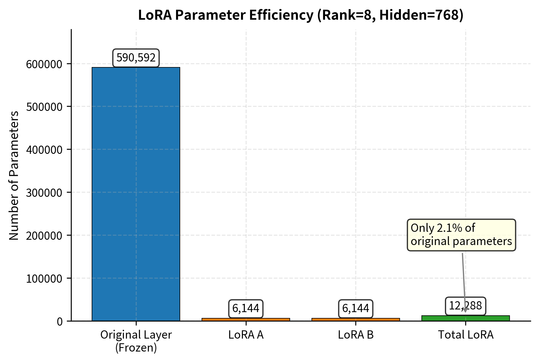
The parameter counts show LoRA's efficiency and explain why this technique is popular for adapting large models. The LoRA adaptation adds a very small fraction of parameters compared to the original dense layer. To understand why, consider the arithmetic: a dense layer with input and output dimensions of 768 has parameters (plus bias). A rank-8 LoRA adds only parameters, representing just over 2% of the original. This ratio improves as model dimensions grow, making LoRA especially effective for large language models where hidden dimensions commonly reach 4096 or higher.
Verifying Initial Behavior
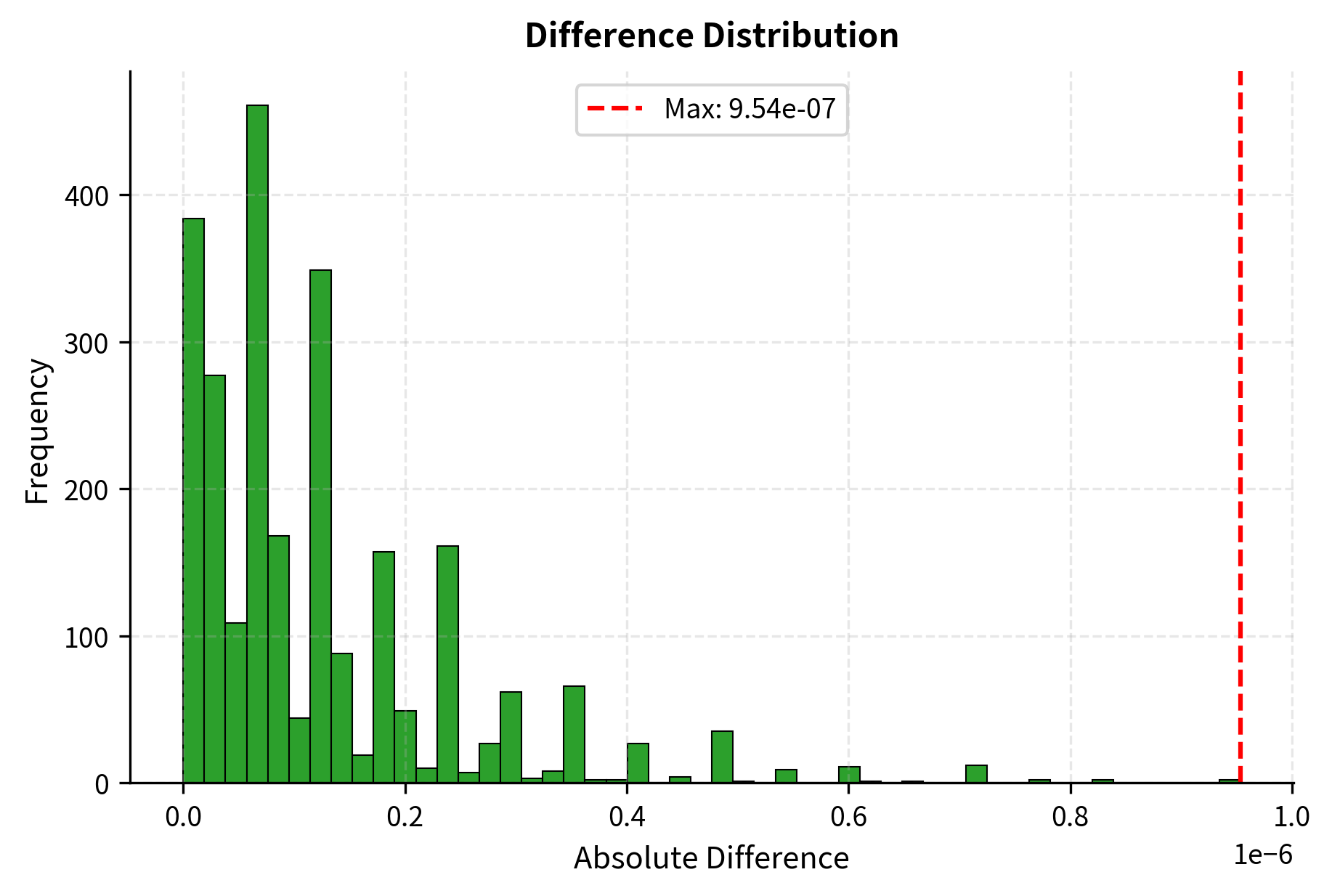
Since is initialized to zeros, the LoRA layer should produce identical outputs to the original layer at initialization. This property is essential for ensuring that applying LoRA doesn't accidentally degrade a model's capabilities before training begins. Let's verify this guarantee holds in practice:
The negligible difference, caused by floating-point precision, confirms that our zero-initialization strategy works. The model will produce exactly the same outputs as before LoRA was applied, giving you confidence that you can add LoRA to any pre-trained model without risking immediate performance degradation.
Key Parameters
Understanding the key parameters for our LoRALinear implementation helps you make informed decisions when applying LoRA to your own models:
- rank: The rank of the low-rank decomposition determines the size of matrices and and thus controls the capacity of the adaptation. Lower ranks use fewer parameters and memory but may limit the complexity of adaptations the model can learn. Higher ranks provide more expressiveness but increase computational cost.
- alpha: The scaling factor controls the magnitude of the adaptation updates relative to the original layer outputs. Higher values make the LoRA contribution more influential, effectively amplifying the learning rate for the adaptation pathway.
- dropout: The probability of zeroing elements in the LoRA path during training, which helps prevent overfitting when fine-tuning on small datasets. This regularization applies only to the adaptation pathway, leaving the frozen base model unaffected.
Integrating LoRA into Transformer Models
Real transformer models contain many linear layers distributed throughout their architecture: the query, key, and value projections in each attention head, the output projection that recombines attention results, and the feed-forward networks that process each position independently. A typical LoRA configuration targets the attention projections, as these capture the most task-relevant transformations by controlling what information the model attends to and how it combines that information.
Applying LoRA to a full model requires identifying and replacing layers without manually editing the architecture. We need an automated approach that can traverse the model's module hierarchy, find layers matching our target criteria, and wrap them with LoRA adapters while preserving the model's structure.
Let's create a utility function that recursively replaces specified linear layers with LoRA versions:
This function implements a recursive traversal strategy that examines every module in the model hierarchy. For each module, it checks whether the module name contains any of the target patterns, allowing flexible specification of which layers to adapt. The function then verifies that the module is actually a linear layer (since LoRA applies specifically to linear transformations), creates a LoRA wrapper around it, and performs the replacement by navigating to the parent module and updating the attribute. This pattern-based approach means you can target layers by their role (like "q_proj" for query projections) rather than their exact position in the model structure.
Let's demonstrate this with a simplified transformer block that contains the essential components found in production models:
Now we can inject LoRA into the attention projections, demonstrating how the injection process affects parameter counts and training behavior:
The model now has the same representational capacity as before, since all original weights are preserved and can contribute to the forward pass. However, only the LoRA parameters are trainable, resulting in a dramatic reduction in the number of parameters that require gradient computation and optimizer state storage. This demonstrates LoRA's core value proposition: the ability to fine-tune large models on limited hardware by concentrating all learning into a small, efficient set of parameters.
The LoRA Training Loop
Training a LoRA-equipped model follows the standard PyTorch training pattern, with one key simplification: the optimizer only needs to handle the LoRA parameters. This means smaller optimizer state memory, faster parameter updates, and reduced gradient computation since gradients don't flow through the frozen base weights.
Let's build a complete training example to illustrate these concepts in action:
Now let's implement a training loop for a simple sequence classification task, which demonstrates how LoRA integrates into a realistic training workflow:
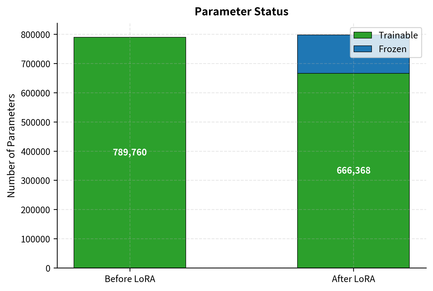
At this stage, all parameters in the model are trainable. This represents the baseline for full fine-tuning, which would require updating every weight in the network. For large models, this baseline represents a significant memory burden since the optimizer must store momentum and variance estimates (in the case of Adam-family optimizers) for every parameter.
After injecting LoRA, the number of trainable parameters drops precipitously. The vast majority of the model, comprising the original weights from embeddings, attention layers, feed-forward networks, and the classifier, is now frozen. Only the small adapter matrices remain trainable. This transformation is what enables LoRA to fine-tune models that would otherwise exceed available memory.
The training loop demonstrates that LoRA integrates naturally with standard PyTorch workflows. The code structure is virtually identical to full fine-tuning, with only two modifications required. First, we inject LoRA into target modules using our utility function. Second, we pass only LoRA parameters to the optimizer, ensuring that gradient updates only apply to the adaptation matrices. Everything else, including the forward pass, loss computation, backpropagation, and optimizer stepping, proceeds exactly as in conventional training.
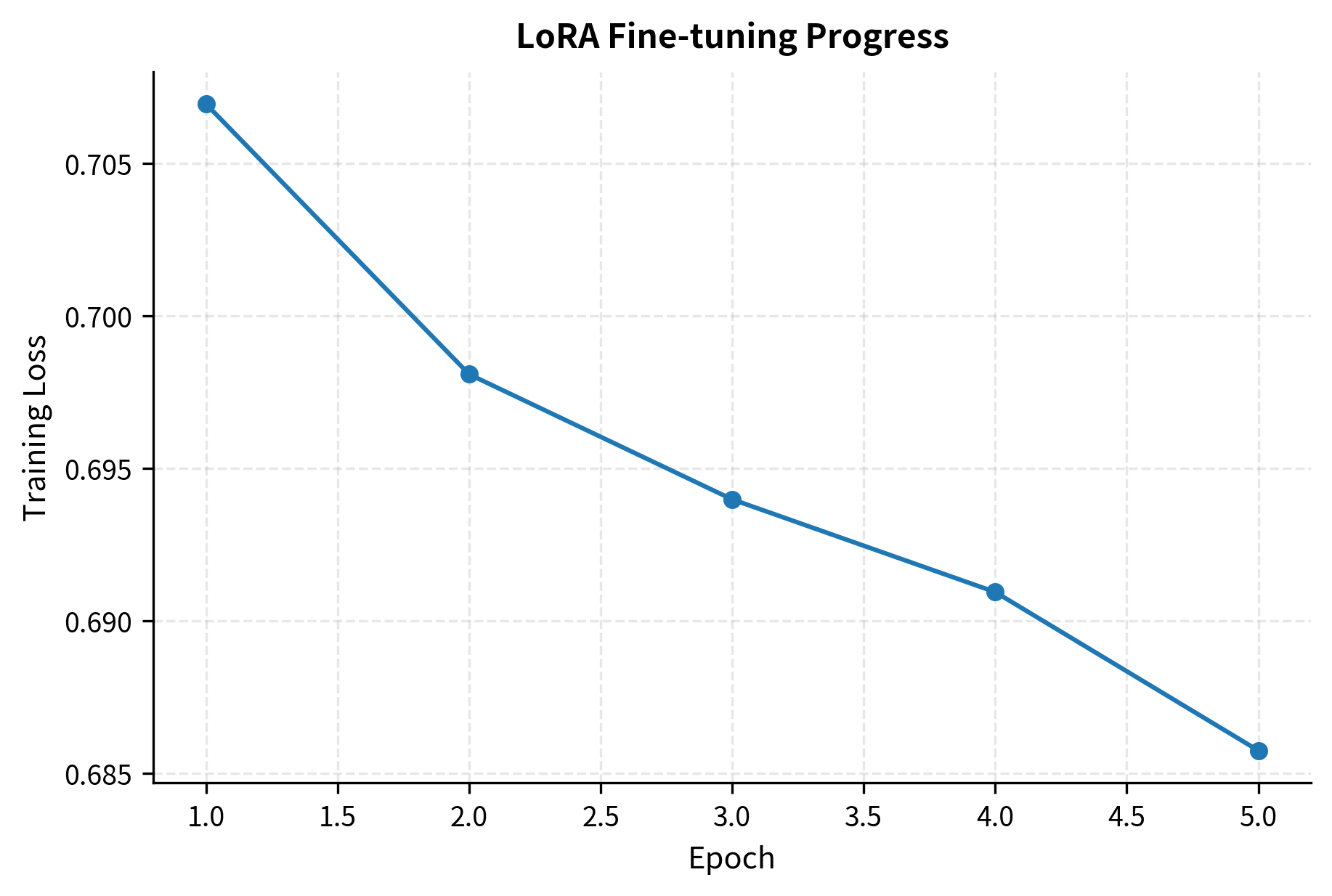
Let's visualize the training progress:
Weight Merging for Efficient Inference
During training, LoRA maintains separate paths for the original weights and the low-rank adaptation. This separation is necessary because we need to keep the original weights frozen while allowing gradients to flow through only the adaptation matrices. However, this dual-path architecture introduces computational overhead during inference: each adapted layer must perform the original matrix multiplication plus the additional low-rank computation.
At inference time, we can merge the LoRA weights back into the base model, eliminating any computational overhead. The merged model produces identical outputs to the unmerged version but requires only a single matrix multiplication per layer:
where:
- : the consolidated weight matrix used for inference
- : the original frozen weight matrix
- : the scaling factor
- : the rank parameter
- : the projection-up matrix
- : the projection-down matrix
- : the effective update matrix computed from the LoRA parameters
This merging relies on the distributive property of linear transformations over addition. Specifically, applying a linear layer with weight and then adding the output of another linear operation with weight is mathematically equivalent to applying a single linear layer with weight . We can verify that the merged weight produces identical outputs to the separate paths through careful mathematical analysis. For an input vector , the forward pass equivalence is derived as follows:
where:
- : the input vector
- : the transpose of the merged weight matrix used in the linear layer
- : the transpose of the original frozen weight matrix
- : the scaling factor
- : the rank parameter
- : the transposes of the adaptation matrices (note the order reversal due to the transpose property)
The final expression shows exactly what our unmerged forward pass computes: the original layer output plus the scaled LoRA contribution . This mathematical equivalence confirms that we can eliminate the computational overhead during inference by using a consolidated weight matrix:
Let's modify our LoRALinear class to handle merged weights in the forward pass, creating a version that can operate in either mode:
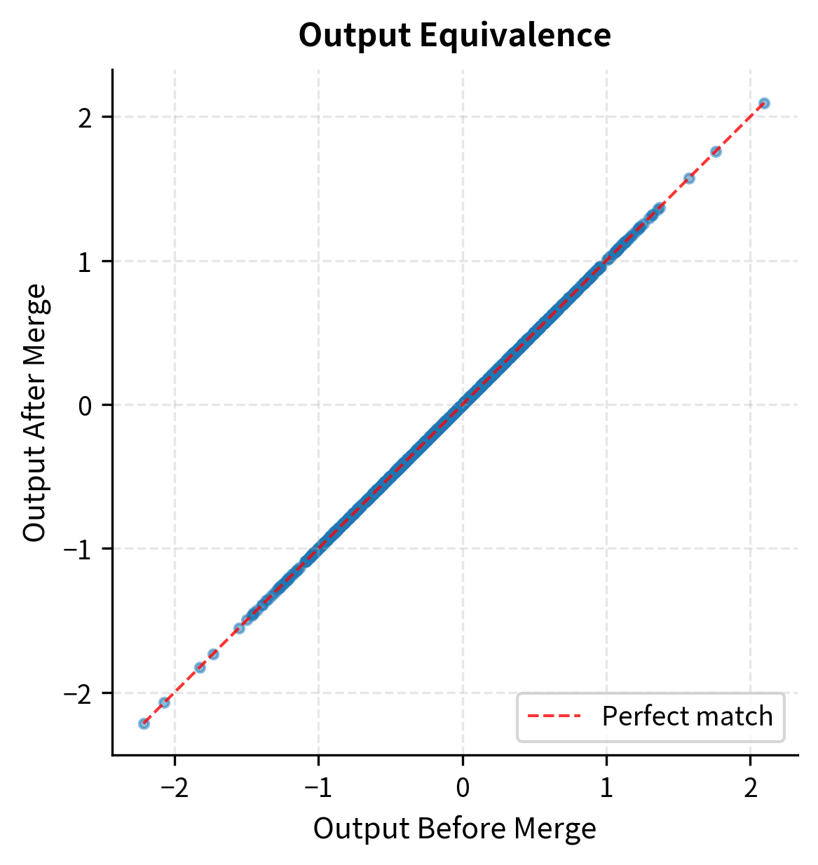
Let's verify that merging produces identical outputs, confirming our mathematical derivation:
The outputs are identical up to floating-point precision, confirming that merged models have zero inference overhead compared to the original architecture. This verification provides confidence that you can deploy merged models in production without worrying about subtle behavioral differences.
Saving and Loading LoRA Weights
For practical deployment, you often want to save only the LoRA weights rather than the full model. This approach enables sharing small adapter files that can be applied to any copy of the base model, creating an efficient ecosystem where you download a large base model once and then apply multiple lightweight adapters for different tasks:
The LoRA checkpoint is orders of magnitude smaller than a full model checkpoint, enabling practical storage and distribution of many task-specific adaptations. You might maintain dozens of LoRA adapters for different tasks while storing just one copy of the base model, dramatically reducing storage requirements compared to maintaining multiple fully fine-tuned model variants.
HuggingFace PEFT Library
While understanding the implementation details is valuable for building intuition and debugging issues, production systems typically use the PEFT (Parameter-Efficient Fine-Tuning) library from HuggingFace. PEFT provides optimized implementations of LoRA and other adaptation methods, with seamless integration into the transformers ecosystem. Using PEFT means you benefit from tested, maintained code that handles edge cases and optimizations you might miss in a custom implementation.
Let's walk through a practical example of fine-tuning a language model with PEFT:
The PEFT library uses a configuration object to specify LoRA hyperparameters, providing a clean interface for customizing the adaptation behavior:
The output shows the dramatic reduction in trainable parameters achieved by PEFT. With just a single function call, the library has identified the target modules, wrapped them with LoRA adapters, and frozen the base weights. Let's examine the modified architecture to understand what changed:
The output confirms that the targeted linear layers have been successfully wrapped with LoRA adapters. These adapters intercept the forward pass, adding the low-rank adaptation path alongside the frozen base computation.
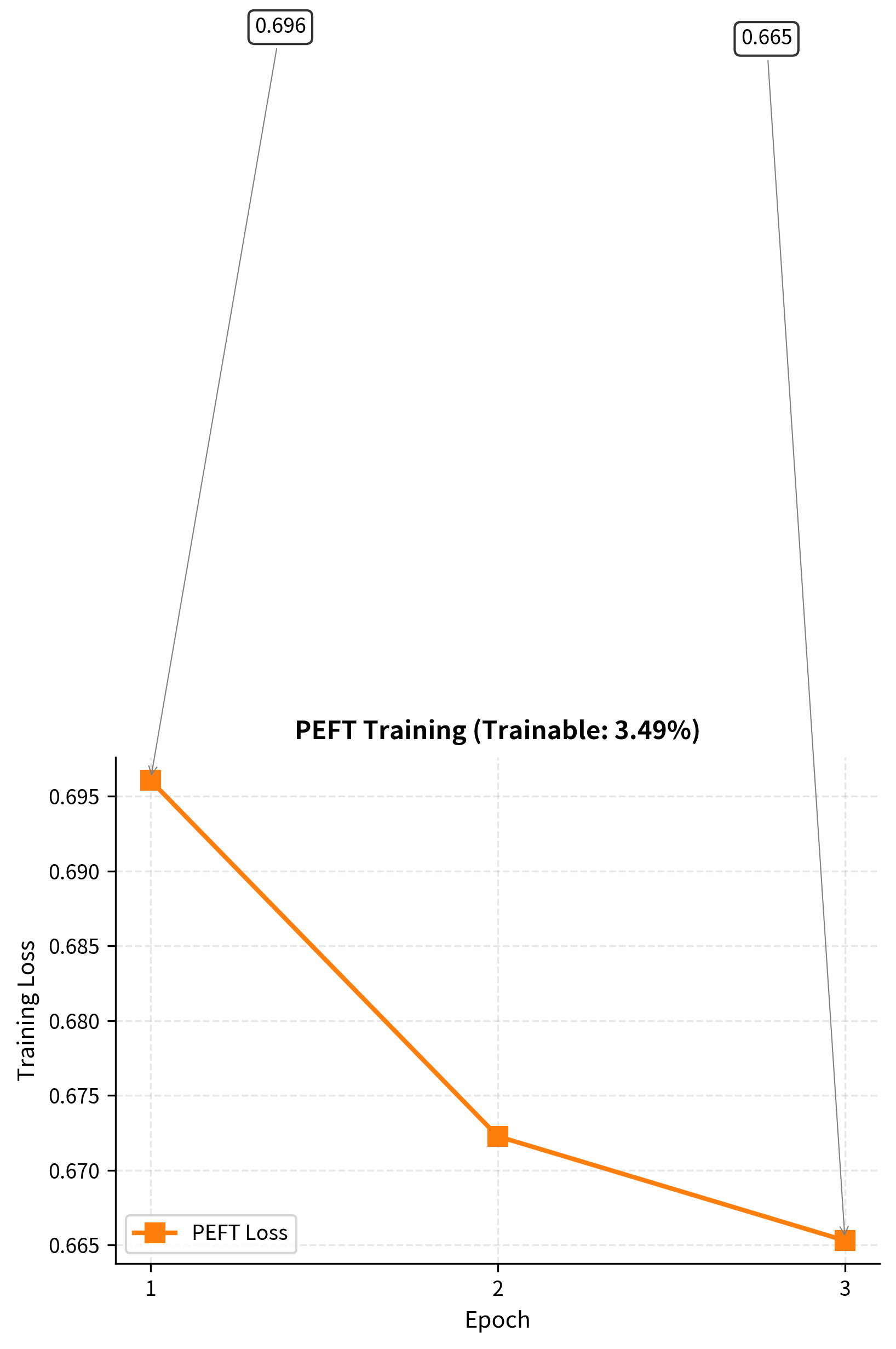
Training with PEFT
Training a PEFT model is identical to training any HuggingFace model. The library handles freezing base weights and updating only LoRA parameters transparently, so your training code requires no special modifications:
The steady decrease in loss shows the model is learning from the dataset. Optimizing just the small set of LoRA parameters is sufficient. This validates the core hypothesis behind LoRA: that task-specific adaptations can be captured in a low-rank subspace.
Saving and Loading PEFT Models
PEFT provides convenient methods for saving only the adapter weights, making it easy to distribute lightweight task-specific adaptations:
The adapter checkpoint is just a few hundred kilobytes, compared to hundreds of megabytes for the full DistilBERT model. This enables practical workflows where you distribute a single base model with many task-specific adapters, allowing you to quickly switch between different capabilities without downloading or storing multiple complete models.
Merging and Unloading
PEFT also supports merging LoRA weights for inference, providing a one-line solution for converting your adapted model into a standard format:
After merging, you have a standard transformer model with no LoRA overhead, suitable for optimized inference pipelines. The merged model can be deployed using any existing serving infrastructure without special handling for LoRA adapters.
Key Parameters
The key parameters for LoraConfig in the PEFT library provide fine-grained control over the adaptation behavior:
- r: The rank of the low-rank decomposition. Lower ranks (4-16) use fewer parameters but may capture less complex adaptations. Higher ranks provide more expressiveness at the cost of increased memory and computation.
- lora_alpha: The scaling factor for LoRA updates. It functions similarly to a learning rate multiplier for the adapters, controlling how strongly the adaptation influences model outputs relative to the frozen base weights.
- target_modules: The specific modules (usually linear layers) to apply LoRA to. Common targets in transformers are query and value projections (
q_lin,v_lin), which control attention patterns. Targeting more modules increases adaptation capacity but also parameter count. - lora_dropout: Dropout probability applied to the LoRA path to prevent overfitting during training, particularly important when fine-tuning on small datasets where the model might memorize rather than generalize.
Limitations and Impact
LoRA implementation brings certain practical constraints that you should understand before applying the technique to your own models and tasks.
The rank fundamentally limits the expressiveness of the adaptation. When the required weight updates truly need full-rank modifications, such as when adapting to a dramatically different domain or learning entirely new capabilities, LoRA may underperform full fine-tuning. The low-rank constraint assumes that the difference between the pre-trained model and the adapted model lives in a low-dimensional subspace, which holds well for many fine-tuning tasks but may break down for more substantial modifications. We'll explore strategies for selecting appropriate rank values in the next chapter on LoRA hyperparameters.
The choice of target modules significantly affects both performance and efficiency. Targeting all linear layers captures the most information and provides maximum flexibility for the adaptation, but it also increases parameter count and training memory proportionally. In practice, attention projections (query and value) provide the best performance-to-parameter ratio for most tasks, as these layers directly control what information the model attends to. However, optimal targeting varies by domain: feed-forward networks may be important for tasks requiring different knowledge representations, while leaving them untouched often works well for stylistic adaptations that primarily change how existing knowledge is expressed.
Memory savings during training come primarily from reduced gradient computation and optimizer states. For an 8-billion parameter model with rank-16 LoRA applied to attention layers, trainable parameters drop to roughly 20 million, about 0.25% of the original count. This dramatic reduction enables fine-tuning on a single consumer GPU that couldn't otherwise hold the optimizer states for full fine-tuning, where Adam requires approximately 16 bytes per parameter (4 bytes each for the parameter, gradient, momentum, and variance estimates).
Inference behavior depends on whether weights are merged. Unmerged LoRA adds latency from the additional matrix multiplications in the low-rank path. For batch sizes of one, which are common in interactive applications like chatbots, this overhead is typically 5-15% depending on the specific model architecture and hardware. Merging eliminates this entirely, but you lose the ability to dynamically switch between adapters or continue training. Many applications use unmerged models during development for flexibility and merge before production deployment.
LoRA's impact on the field has been substantial and far-reaching. Before LoRA, fine-tuning large language models was effectively limited to organizations with significant compute resources, creating a divide between those who could customize models and those who couldn't. LoRA democratized adaptation, enabling you with single GPUs to customize billion-parameter models for your specific needs. This accessibility accelerated the development of domain-specific applications across medicine, law, education, and countless other fields. The technique also spawned an ecosystem of shared adapters for various tasks, where you contribute and download small adapter files rather than full model weights. Subsequent techniques like QLoRA, which we'll cover in an upcoming chapter, push these efficiency gains even further by combining LoRA with quantization to enable fine-tuning on even more constrained hardware.
Summary
This chapter transformed the mathematical concepts from the previous chapter into working implementations. The key implementation components are:
-
LoRA Module Design: A LoRALinear class wraps existing linear layers, adding parallel low-rank matrices and while keeping original weights frozen. Zero-initialization of ensures the model starts identical to the pre-trained version.
-
Model Integration: A recursive injection function identifies target modules (typically attention projections) and replaces them with LoRA-wrapped versions, automatically freezing base weights.
-
Training Loop: Standard PyTorch training, but the optimizer receives only LoRA parameters. Memory savings come from reduced gradient computation and optimizer state storage.
-
Weight Merging: At inference time, produces a standard model with zero overhead. This can be reversed for continued training.
-
PEFT Library: HuggingFace's PEFT provides production-ready LoRA with
LoraConfigfor configuration,get_peft_modelfor wrapping, andsave_pretrained/merge_and_unloadfor deployment workflows.
The next chapter examines how to select LoRA hyperparameters, including rank, alpha, target modules, and their interactions, to optimize for your specific task and computational constraints.
Quiz
Ready to test your understanding? Take this quick quiz to reinforce what you've learned about LoRA implementation.

Comments