

Learn QLoRA for fine-tuning large language models on consumer GPUs. Master NF4 quantization, double quantization, and paged optimizers for 4x memory savings.

This article is part of the free-to-read Language AI Handbook
Choose your expertise level to adjust how many terms are explained. Beginners see more tooltips, experts see fewer to maintain reading flow. Hover over underlined terms for instant definitions.
Here is the corrected document:
execute: cache: true jupyter: python3
QLoRA
In the previous chapters, we explored LoRA's elegant approach to parameter-efficient fine-tuning: training small, low-rank adapter matrices while keeping the base model frozen. This dramatically reduces the number of trainable parameters, but there's a catch. Even though we only train the adapters, we still need to load the entire base model into memory to compute forward passes. For a 7-billion parameter model stored in 16-bit precision, that's still 14 GB of GPU memory just for the frozen weights, before accounting for activations, gradients, or optimizer states.
QLoRA (Quantized LoRA) solves this problem by storing the frozen base model in 4-bit precision while training LoRA adapters in full precision. This isn't simply applying standard 4-bit quantization; it introduces several innovations that preserve model quality while achieving dramatic memory reductions. A 65-billion parameter model that would require 130 GB of memory in FP16 can be fine-tuned on a single 48 GB GPU using QLoRA, with no loss in final performance.
The key innovations behind QLoRA are a new 4-bit data type called NormalFloat (NF4) that's optimized for normally distributed weights, double quantization to minimize storage overhead, and paged optimizers that gracefully handle memory spikes. Together, these techniques enable fine-tuning models that were previously out of reach.
The Memory Bottleneck
Before diving into QLoRA's solutions, let's understand exactly where memory goes during fine-tuning. When training with standard LoRA, GPU memory is consumed by several components, each contributing to the overall memory footprint in different ways. Understanding this breakdown is essential because it reveals why simply reducing trainable parameters isn't enough to make large models accessible.
The base model weights dominate memory for large models. Even frozen, these weights must reside in GPU memory for forward passes. The reason is straightforward: every forward pass requires matrix multiplications between activations and weights, and these operations happen on the GPU. Moving weights from CPU to GPU for each forward pass would create an unacceptable bottleneck. In FP16, each parameter requires 2 bytes of storage:
where:
- : the total number of parameters in the base model
- : the size in bytes of a single parameter in half-precision (FP16 or BF16)
For a 7B parameter model, that's 14 GB. For a 70B model, that's 140 GB. These numbers represent a hard floor on memory requirements regardless of any other optimizations we might apply to the training process.
LoRA adapter weights are relatively small. With typical settings (rank 8-64 targeting attention layers), the adapters constitute roughly 0.1-1% of base model parameters. This is precisely what makes LoRA attractive: the trainable component is tiny compared to the base model.
Gradients are only computed for LoRA parameters during backpropagation, since the base model is frozen. This is LoRA's key memory advantage. In full fine-tuning, gradients for every parameter must be stored, effectively doubling the memory requirement during training. LoRA eliminates this cost for the vast majority of parameters.
Optimizer states for Adam-based optimizers store momentum and variance estimates for each trainable parameter. In FP32, this requires 8 bytes per trainable parameter (4 for momentum, 4 for variance). Again, because LoRA only trains a small number of parameters, this cost remains manageable.
Activations must be stored during the forward pass for gradient computation during backpropagation. This scales with batch size and sequence length. Gradient checkpointing can reduce this cost by recomputing activations during the backward pass, trading computation for memory.
The bottleneck is clear: even with LoRA's efficient training, the base model's frozen weights consume enormous memory. QLoRA directly attacks this by storing those weights in 4-bit precision, a 4× reduction compared to FP16. This insight, that we can dramatically compress the frozen weights without harming the training process, is the foundation of the entire QLoRA approach.
Quantization Fundamentals
Quantization maps high-precision values to a smaller set of discrete levels. For neural network weights, the goal is to reduce storage and computation costs while minimizing the accuracy loss from this approximation. To understand why this works at all, consider that neural networks are remarkably robust to noise. Small perturbations to weights typically produce small changes in outputs, which means we have room to introduce controlled approximation errors.
The process of mapping continuous or high-precision values to a finite set of discrete levels. In the context of neural networks, quantization typically converts 32-bit or 16-bit floating-point weights to lower-precision formats like 8-bit integers or 4-bit values.
Uniform Quantization
The simplest approach is uniform quantization, where the value range is divided into equally-spaced bins. This approach treats all parts of the value range as equally important, allocating the same precision to every region. To quantize a tensor to bits (yielding levels), we first normalize the weights to the range and then scale them to the integer range . The normalization step ensures that all weights fall within a predictable range, while the scaling step maps these normalized values to discrete integer codes that can be stored efficiently. The calculation is:
where:
- : the resulting quantized integer tensor
- : the input high-precision weight tensor
- : the minimum value in the input tensor
- : the maximum value in the input tensor
- : the bit-width used for quantization
- : the maximum integer value representable with bits
The term shifts and scales the weights so that the minimum value maps to 0 and the maximum maps to 1. Multiplying by then stretches this unit interval to span the full range of representable integers. The rounding operation introduces quantization error by snapping each continuous value to its nearest discrete level.
Dequantization reverses this process, reconstructing an approximation of the original weights from the quantized codes:
where:
- : the reconstructed high-precision weight tensor
- : the quantized integer tensor
- : the quantization constants (min and max values) stored alongside the weights
- : the bit-width used for quantization
Notice that we must store and alongside the quantized weights. Without these constants, we cannot recover the original scale and offset. This is a common pattern in quantization: we trade most of the precision for storage savings while keeping a small amount of metadata to enable reconstruction.
Uniform quantization works reasonably well for uniformly distributed data, but neural network weights are decidedly not uniform. As we'll see, this mismatch creates unnecessary quantization error.
Block-wise Quantization
Computing a single scale for an entire weight matrix is problematic because outlier values stretch the quantization range, wasting precision on unused regions. Imagine a weight matrix where most values lie between -0.5 and 0.5, but a few outliers reach ±3.0. Uniform quantization must spread its limited precision across the entire [-3.0, 3.0] range, even though most of this range is sparsely populated. The densely populated central region ends up with coarse granularity, leading to large quantization errors for the majority of weights.
Block-wise quantization addresses this by dividing weights into blocks of size (typically 64 or 128 elements) and computing separate quantization constants for each block. Within each block, the local minimum and maximum determine the quantization range. This allows each block to adapt to its own value distribution, placing precision where it's actually needed.
This improves accuracy but introduces overhead: we must store scaling factors in addition to the quantized weights. For 64-element blocks with FP32 scales, that's an additional 0.5 bits per parameter. This overhead represents the cost of adaptive precision allocation. The accuracy improvement typically outweighs this cost, but as we'll see, QLoRA introduces techniques to minimize even this overhead.
The NormalFloat Data Type
QLoRA's first innovation is recognizing that neural network weights follow approximately normal distributions. This insight enables a quantization scheme that places more precision where the density is highest. Rather than treating all value ranges as equally important, NormalFloat allocates quantization levels according to where weights actually concentrate.
Why Normal Distributions Matter
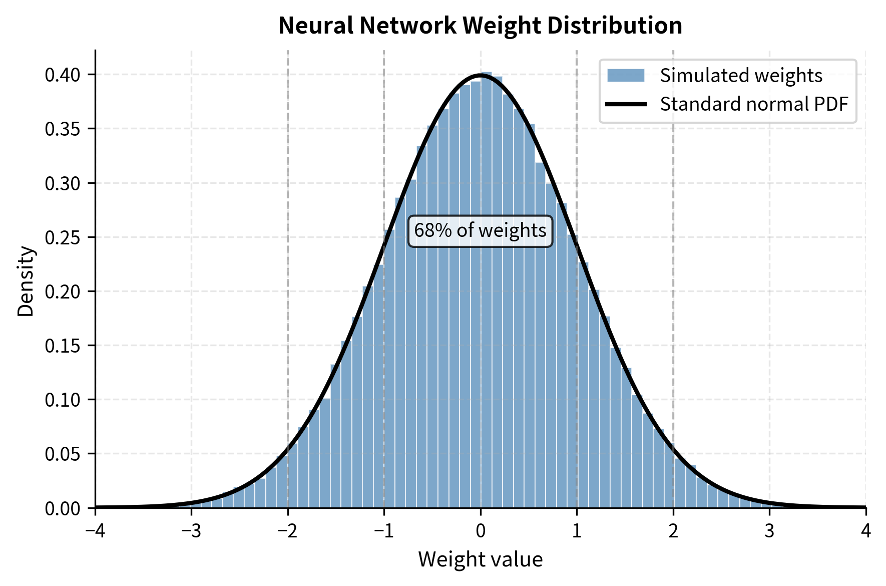
When we initialize neural networks using methods like Xavier or Kaiming initialization, weights are drawn from normal distributions. These initialization schemes are designed to maintain stable gradient flow through deep networks, and they achieve this by carefully controlling the variance of each layer's weights. Training updates through gradient descent tend to maintain this approximate normality, because gradient updates are themselves sums of many small contributions, and sums of random variables tend toward normality by the central limit theorem. Let's verify this empirically:
The high p-value confirms that the weights follow a normal distribution, while the mean and standard deviation align with the initialization parameters. This normality assumption is the foundation for the NormalFloat data type. If we know in advance what distribution our data follows, we can design a quantization scheme specifically optimized for that distribution.
Quantile Quantization
For normally distributed data, uniform quantization is inefficient. Many quantization levels fall in the distribution's tails where few values exist, while the dense center region has insufficient precision. Consider what happens with 16 uniformly spaced levels across the range [-3, 3]: each level covers an interval of width 0.375. But for a standard normal distribution, approximately 68% of values fall within one standard deviation of the mean, packed into just 16% of the total range. Uniform quantization wastes most of its levels on the sparse tails.
NormalFloat uses quantile quantization, a fundamentally different approach. The quantization levels are placed at equal quantiles of the standard normal distribution. For 4-bit quantization with 16 levels, each level corresponds to a region containing exactly of the probability mass. This ensures that each quantization bin is equally likely to be used, maximizing the information content of each bit.
The quantile function (inverse CDF) of the standard normal distribution gives us these boundaries. The quantile function returns the value such that a standard normal random variable has probability of being less than :
where:
- : the value of the -th quantization boundary
- : the inverse cumulative distribution function (quantile function) of the standard normal distribution
- : the index of the boundary
- : the total number of quantization bins (determined by the bit-width )
For example, with 16 bins, we compute boundaries at probabilities 0, 1/16, 2/16, ..., 15/16, 1. The boundary between bins 7 and 8 falls at the median (probability 0.5), which for a standard normal is exactly 0. The boundaries spread out in the tails and cluster tightly near zero, precisely matching where the probability density is highest.
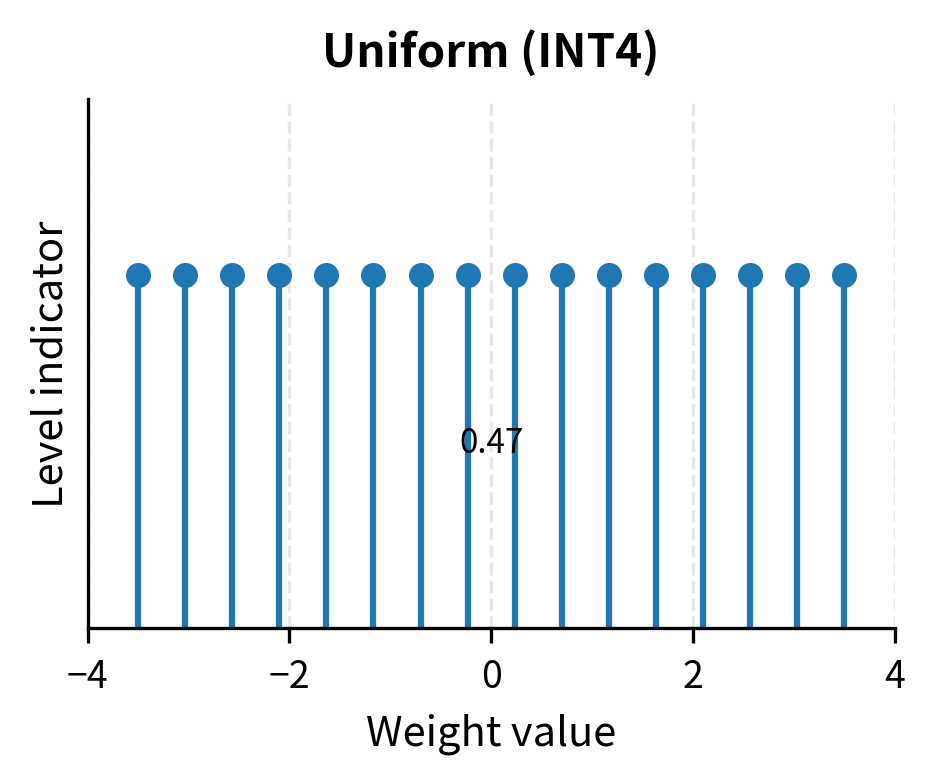
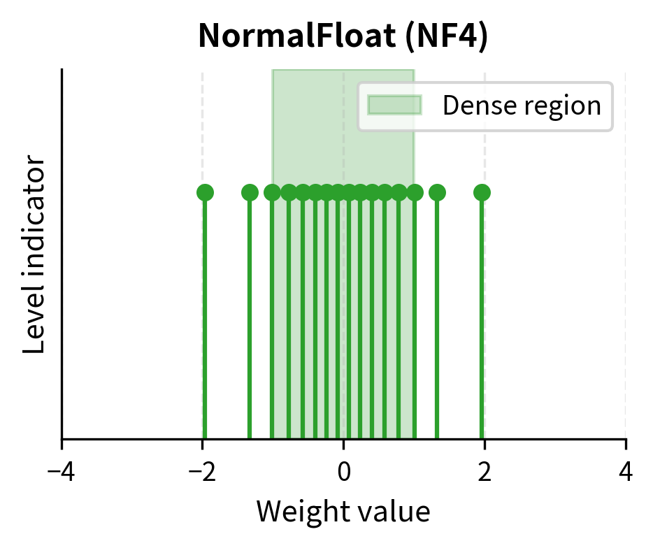
Notice how the levels are more densely packed near zero where most weight values concentrate, and more sparse in the tails. The spacing between levels 7 and 8 (which straddle zero) is much smaller than the spacing between levels 0 and 1 (in the far left tail). This is the key advantage of NF4 over uniform INT4: precision is allocated according to need rather than uniformly.
Visualizing the Difference
Let's compare uniform and NF4 quantization for normally distributed data:
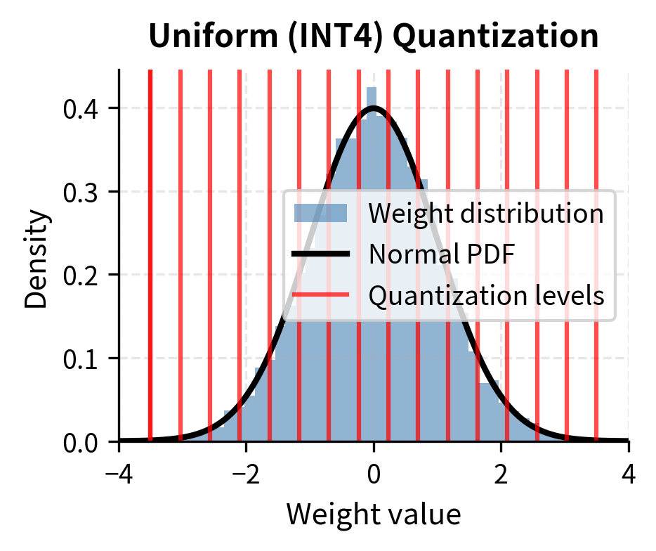
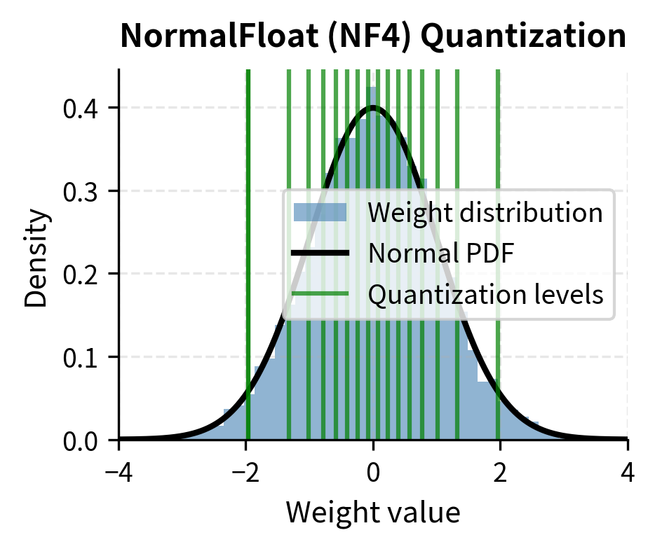
The uniform scheme wastes quantization levels in the sparse tails while providing coarse granularity where it matters most. NF4 allocates precision according to where values actually occur. The visual difference is striking: uniform levels appear evenly distributed regardless of the underlying data, while NF4 levels cluster where the histogram is tallest.
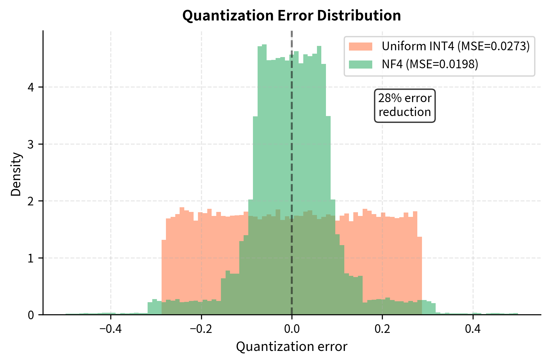
Quantization Error Comparison
Let's measure the reconstruction error for both approaches:
NF4's information-theoretic optimality for normally distributed data translates to substantially lower quantization error. This seemingly technical improvement has major practical implications: lower quantization error means the 4-bit model behaves more like the original FP16 model, preserving capability during fine-tuning. Every reduction in quantization error translates directly to better preservation of the knowledge encoded in the original model weights.
Double Quantization
Block-wise quantization requires storing a scaling factor for each block. These scaling factors enable each block to adapt to its local value distribution, but they come with a storage cost. With 64-element blocks and FP32 scales, the overhead per parameter is:
where:
- : the memory overhead per parameter due to storing scales
- : the size of a single scaling factor in bits (32 for FP32)
- : the number of weights per quantization block (typically 64)
This formula captures the fundamental trade-off in block-wise quantization. Each 64-element block requires one 32-bit scaling factor, so the overhead per element is simply the scale size divided by the block size. For a 70B parameter model, this overhead alone requires 4.4 GB of memory, which is a significant fraction of the memory we're trying to save through quantization.
QLoRA's second innovation is double quantization: quantizing the quantization constants themselves. The key insight is that the scaling factors, while necessary for accurate reconstruction, are themselves just numbers that can be compressed.
The Approach
The scale factors across blocks form their own distribution. Since each scale represents the range of values in a block of normally distributed weights, these scales tend to be positive numbers clustered around a characteristic value determined by the layer's weight statistics. We can apply a second round of quantization to these scales:
- First quantization: Quantize weight blocks using NF4 with FP32 scales
- Second quantization: Quantize the FP32 scales to 8-bit with a single global scale
The scales are typically positive values (since we normalize weights to have unit variance before quantization), so 8-bit unsigned integers work well. Using 256 levels for the scales provides enough precision to avoid meaningful accuracy loss while reducing storage by 4×.
The minimal Mean Squared Error (MSE) confirms that 8-bit quantization preserves the scale information with high accuracy. This suggests we can safely compress the scales without degrading model performance. The error is so small because the scales vary smoothly across blocks, making them well-suited to quantization with many levels.
Memory Savings from Double Quantization
Let's calculate the total memory reduction. The overhead calculation changes because we now store 8-bit scales instead of 32-bit scales, with one additional 32-bit global scale per tensor:
Double quantization reduces the scale storage overhead by 75%, from 0.5 bits per parameter to 0.125 bits per parameter. The quantization error introduced to the scales is negligible since we're using 256 levels and the scales vary smoothly. This reduction might seem small in percentage terms, but for a 70B model, it saves over 3 GB of memory, which can make the difference between fitting on a GPU and not fitting.
QLoRA Architecture
With NF4 and double quantization in hand, let's see how QLoRA combines these with LoRA for end-to-end fine-tuning. The architecture maintains the core LoRA principle of training small adapters while keeping the base model frozen, but adds a quantization layer that dramatically reduces the memory footprint of those frozen weights.
Forward Pass
During the forward pass, QLoRA dequantizes the base model weights on-the-fly and adds the LoRA contribution. The key insight is that we never need to store the full-precision weights in GPU memory. We only need them for the brief moment when we perform each layer's matrix multiplication:
where:
- : the output activation tensor
- : the input activation tensor
- : the base model weights, dequantized from 4-bit storage to 16-bit computation precision
- : the LoRA down-projection matrix (projects inputs to the low-rank dimension )
- : the LoRA up-projection matrix (projects from back to the output dimension)
- : the low-rank update term added to the weights (matrix multiplication of and )
The dequantization happens in GPU registers during matrix multiplication, so the full-precision weights never materialize in GPU memory. This is the key insight that enables memory savings: we store weights in 4 bits but compute in higher precision. The computational cost of dequantization is small compared to the matrix multiplication itself, and modern GPU kernels can fuse the dequantization with the multiply-accumulate operations.
Backward Pass
Gradients flow only through the LoRA adapters and . The quantized base weights remain frozen and require no gradient computation. This is identical to standard LoRA, except the forward pass uses dequantized weights. The backward pass sees no additional complexity from quantization because we don't need to differentiate through the quantization operation. The frozen weights are treated as constants, and gradients are computed only with respect to the trainable adapter parameters.
Precision Hierarchy
QLoRA uses a precision hierarchy that balances memory and accuracy. Different components use different precisions based on their roles in training:
- Base model weights: 4-bit NF4 (storage) → BF16 (computation)
- LoRA adapters: BF16 (storage and computation)
- Gradients: BF16 for LoRA parameters only
- Optimizer states: FP32 (or 8-bit) for LoRA parameters only
The LoRA adapters remain in full precision because they're trainable and small. Quantizing the adapters would introduce noise into the gradient updates, potentially destabilizing training. Since the adapters represent only a tiny fraction of total parameters, keeping them in full precision has negligible memory cost.
The optimizer states use FP32 to maintain training stability, but since they only exist for the tiny LoRA parameters, the memory cost is negligible. The 8-bit optimizer option provides additional savings for situations where memory is extremely constrained.
Memory Savings Analysis
Let's quantify QLoRA's memory advantages with concrete numbers for different model sizes.
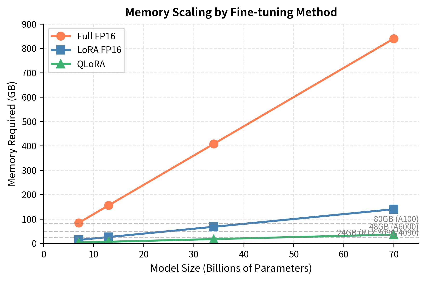
Let's visualize the memory breakdown for a 70B model:
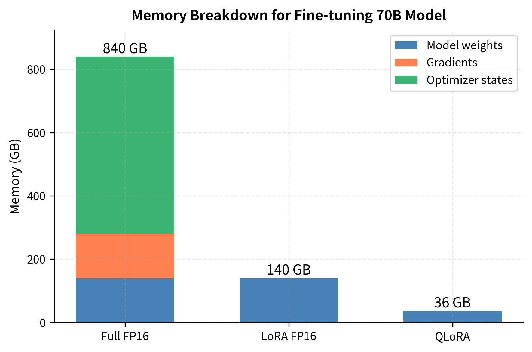
The visualization reveals that for both full fine-tuning and standard LoRA, the base model weights dominate memory usage. QLoRA's 4-bit quantization directly addresses this bottleneck, reducing model memory from 140 GB to approximately 36 GB. The gradient and optimizer state contributions remain small for LoRA and QLoRA because only the adapter parameters require these training artifacts.
Paged Optimizers
QLoRA introduces one additional innovation beyond quantization: paged optimizers using NVIDIA's unified memory. During training, memory usage can spike unpredictably due to long sequences or unusual batch compositions. These spikes are difficult to predict in advance because they depend on the specific data being processed. When GPU memory is exhausted, the training process crashes.
Paged optimizers handle this gracefully by automatically transferring optimizer states between GPU and CPU memory as needed. When GPU memory runs low, inactive optimizer states are paged to CPU memory. When they're needed for an update, they're paged back. This enables training to continue even when memory demand temporarily exceeds GPU capacity, at the cost of some speed overhead during memory transfers.
This technique is particularly valuable for QLoRA because the memory savings already put us at the edge of what fits on a given GPU. We're deliberately operating close to the memory limit to maximize model size. Paged optimizers provide a safety margin against memory spikes that would otherwise crash training.
Implementation with bitsandbytes
The bitsandbytes library provides efficient CUDA kernels for 4-bit operations, and the peft library integrates these with LoRA. Let's walk through a practical QLoRA setup.
The key parameters in BitsAndBytesConfig are:
- load_in_4bit: Enables 4-bit quantization when loading the model
- bnb_4bit_quant_type: Specifies NF4 rather than uniform INT4
- bnb_4bit_compute_dtype: Sets the dtype for dequantized computation
- bnb_4bit_use_double_quant: Enables quantization of the quantization constants
Loading a Quantized Model
The prepare_model_for_kbit_training function performs several important operations:
- Enables gradient checkpointing to reduce activation memory
- Freezes all quantized layers
- Casts layer norms to FP32 for training stability
Adding LoRA Adapters
For a 7B model with rank-16 LoRA targeting attention projections, typically less than 1% of parameters are trainable.
Training Configuration
The paged_adamw_8bit optimizer combines two memory-saving techniques: 8-bit Adam (which quantizes optimizer states) and paged memory management. The 8-bit optimizer states provide an additional 2× reduction for the already-small LoRA optimizer states.
Inference with Merged Weights
After training, you can either use the adapter on top of the quantized model, or merge and export to full precision:
Limitations and Impact
QLoRA represented a breakthrough in democratizing LLM fine-tuning. Before QLoRA, fine-tuning a 65B parameter model required multiple high-end GPUs with hundreds of gigabytes of combined memory. QLoRA made this possible on a single consumer or cloud GPU, bringing fine-tuning capabilities to users who previously couldn't afford the hardware requirements.
The memory savings are genuine and substantial. The original QLoRA paper demonstrated fine-tuning LLaMA-65B on a single 48GB GPU while matching 16-bit fine-tuning quality across diverse tasks. This wasn't just a proof-of-concept; the resulting Guanaco models achieved 99.3% of ChatGPT's performance on the Vicuna benchmark while being trained in under 24 hours on a single GPU.
However, QLoRA involves meaningful trade-offs. The primary cost is training speed: 4-bit operations require dequantization before computation, adding overhead to every forward pass. Training throughput is typically 20-40% lower than equivalent FP16 training. If you have sufficient GPU memory, standard LoRA in FP16 remains faster.
The quality preservation, while impressive, isn't perfect. Some tasks show small degradations compared to full-precision fine-tuning, particularly when the base model's quantization error interacts poorly with the task distribution. Fine-grained reasoning tasks occasionally show more sensitivity. The practical solution is simply to evaluate on your specific task; for most applications, the quality difference is negligible.
There's also a subtle interaction between quantization and LoRA rank. Because the base model has quantization noise, the LoRA adapters must learn to compensate for this noise in addition to adapting to the new task. We might find that slightly higher ranks (e.g., 32-64 instead of 8-16) work better with QLoRA than with standard LoRA, though this is task-dependent.
The broader impact of QLoRA extends beyond pure memory savings. By making fine-tuning accessible on consumer hardware, it enabled rapid experimentation and iteration that was previously impossible. The technique contributed to the explosion of open-source fine-tuned models in 2023-2024. Many of the LoRA variants we'll explore in upcoming chapters, like AdaLoRA, build on insights from QLoRA about the interaction between quantization and adaptation.
Summary
QLoRA combines three innovations to enable fine-tuning of massive language models on consumer hardware:
4-bit NormalFloat (NF4) quantization exploits the fact that neural network weights follow approximately normal distributions. By placing quantization levels at equal quantiles of the normal distribution rather than uniformly, NF4 minimizes reconstruction error for typical weights. This information-theoretically optimal quantization preserves model capability far better than naive 4-bit approaches.
Double quantization addresses the overhead of storing per-block scaling factors. By quantizing the FP32 scales to 8-bit integers, the storage overhead drops from 0.5 bits per parameter to 0.125 bits per parameter, a 75% reduction. The minimal additional quantization error is well worth the memory savings.
Paged optimizers provide graceful handling of memory spikes by automatically moving optimizer states between GPU and CPU memory. This prevents training crashes when memory demand temporarily exceeds capacity.
Together, these techniques reduce the memory footprint of base model weights by approximately 4× while keeping trainable LoRA adapters in full precision. A 70B parameter model that requires 140 GB in FP16 fits in approximately 36 GB with QLoRA. This brings fine-tuning of the largest open models within reach of a single high-end consumer GPU.
The key insight behind QLoRA is that we can tolerate approximate computation during the forward pass (via quantization) while maintaining precise gradient updates to the adapters. The frozen base model serves as a noisy but useful initialization; the small, full-precision adapters learn the task-specific adjustments that matter for the final application.
Quiz
Ready to test your understanding? Take this quick quiz to reinforce what you've learned about QLoRA and efficient fine-tuning of large language models.

Comments